S2Former: Parallel Spectral–Spatial Transformer for Hyperspectral Image Classification

Abstract

Due to their excellent representation talent in local features, the convolutional neural network (CNN) has achieved favourable performance in hyperspectral image (HSI) classification tasks. Nevertheless, current CNN models exhibit a marked flaw: they are hard to model the dependencies in long-range distanced positions. This flaw becomes more problematic for the HSI classification task, which targets extracting more discriminative features in local and global dimensions from limited samples. In this paper, we introduce a spatial–spectral transformer (S2Former), which explores spatial and spectral feature extraction in a dual-stream framework for HSI Classification. S2Former, which consists of a spatial transformer and a spectral transformer in parallel branches, extracts the discriminative feature in spatial and spectral dimensions. More specifically, we propose multi-head spatial self-attention to capture the long-range spatial dependency of non-adjacent HSI pixels in a spatial transformer. In the spectral transformer, we propose multi-head covariance spectral attention to mine and represent spectral signatures by computing covariance-based channel maps. Meanwhile, the local activation feed-forward network is developed to complement local details. Extensive experiments conducted on four publicly available datasets indicate that our S2Former achieves state-of-the-art performance for the HSI classification task.

1. Introduction

Hyperspectral imaging measures the reflected solar radiation of land cover objects over dozens to hundreds of spectra. The hyperspectral image (HSI) collects rich and detailed spectral information, effectively reflecting the subtle spectral difference of different objects. This provides significant potential in Earth observation missions, such as land cover mapping [1], precision agriculture [2], land cover classification [3], environmental monitoring [4], and mineral exploration [5]. Several hyperspectral image data processing techniques have been explored, such as denoising [6,7], unmixing [8,9], super- resolution [10,11,12,13], target detection [14,15], change detection [16], and classification [17,18,19,20,21]. Among these techniques, HSI classification has attracted more attention.

The main challenge of HSI classification is how to extract enough discriminative features from limited and insufficient samples. CNN has exhibited potential in learning generalisable features from samples. Thus, it has been widely exploited to customise HSI classifiers. To tackle the above challenge, the CNN-based solutions are mainly grouped into two categories. First, deeper network structures are proposed to extract more delicate features from the limited training samples. Lee et al. [22] proposed a contextual deep CNN (CDCNN) for extracting contextual spatial–spectral features. In [23], a regularised deep feature extraction (FE) method is proposed to effectively solve the common problems of insufficient and unbalanced training samples for HSI. Residual Network (ResNet) [24] and Dense Convolutional Network (DenseNet) [25] are designed to relieve the training stress of deep model. Based on the ResNet, SSRN [26] was proposed, which exploits the deep model to improve classification accuracy. Similarly, FDSSC [27] was designed based on the DenseNet framework to capture spectral–spatial features. Second, the attention mechanism is introduced to refine and reweight the extracted spatial and spectral features. Attention mechanism, a dynamic weight adjustment operation on features, is widely used to optimise feature extraction and refine features. Spectral-wise attention (MSDN-SA) [28] was proposed to enhance the discriminatory ability of the model for spectral features. Channel-wise attention and spatial-wise attention were introduced [29,30] to refine spatial and spectral features and achieve outstanding classification results.

However, the CNN models only model and analyse the limited receptive field and, thus, ignore the global contextual information without the ability of modeling long-range location dependency. As applied to the high-dimensional hyperspectral data, the inherent bias of CNN is magnified. The inadequate global representation ability led to ignoring global spatial and global spectral features, which most likely contain discriminative features. Even for CNN-based methods that are involved with self-attention modules, they still fail to simultaneously constrain the global spatial information and global spectral information of input HSI cubes.

A transformer has excellent performance on most computer vision tasks. It relies on the self-attention mechanism to model global contextual information, simulate the global receptive field, and capture the global information and long-term dependence of samples. This feature greatly alleviates the above-mentioned limitations of using CNN-based methods to complete HSI classification tasks. ViT [31] is the earliest transformer architecture proposed for use in the field of computer vision and has achieved better results than convolutional neural networks. Inspired by ViT, Xue et al. [32] developed a novel deep hierarchical vision transformer (DHViT) to extract long-term spectral dependencies and hierarchical features. Zhao et al. [33] proposed a Convolutional Transformer Network (CTN). The proposed Convolutional Transformer (CT) blocks solved the problem of weak local feature extraction by the transformer and effectively captured the local–global features of HSI patches. A new backbone network named SpectralFormer [34] combines the advantages of transformer and CNN, aiming to learn local spectral feature representation and feature transfer between shallow and deep layers. Song et al. [35] designed a Bottleneck Spatial–Spectral Transformer (BS2T) to describe the dependencies between HSI pixels over long-term locations and bands. HSI-Mixer [36] uses a simple CNN architecture to simulate the function of transformer, reconsiders the significant inductive bias of convolution. A hybrid measurement-based linear projection and spatial and spectral mixer blocks are constructed to implement spatial–spectral feature fusion and decomposition, respectively. However, these transformer-based classifiers just introduce the self-attention mechanism to capture global features. Self-attention is a special attention mechanism that only considers the adaptability in the spatial dimension but ignores the adaptability in the channel dimension, which is also important for HSI classification task. For transformer-based HSI classifiers, it is essential to design the self-attention mechanism separately tailored for spatial and spectral dimensions.

In this article, we aim to develop a novel transformer-based dual-branch network architecture, parallel spatial–spectral transformer (S2Former for short), to achieve high-performance HSI classification by extracting discriminative features in both spatial and spectral dimensions with tailored self-attentions. S2Former consists of a spatial transformer and spectral transformer in parallel branches, emphasising the global spectral information and the spatially global context individually. Specifically, the spatial transformer exploits the multi-head spatial self-attention (MSSA) and local activation feed-forward network to learn the spatially global context and local signals. The spectral transformer equips multi-head covariance spectral attention (MCSA) to model the contextualised global relationships between spectra and capture the subtle spectral discrepancies.

The main contributions can be concluded as follows.

1.

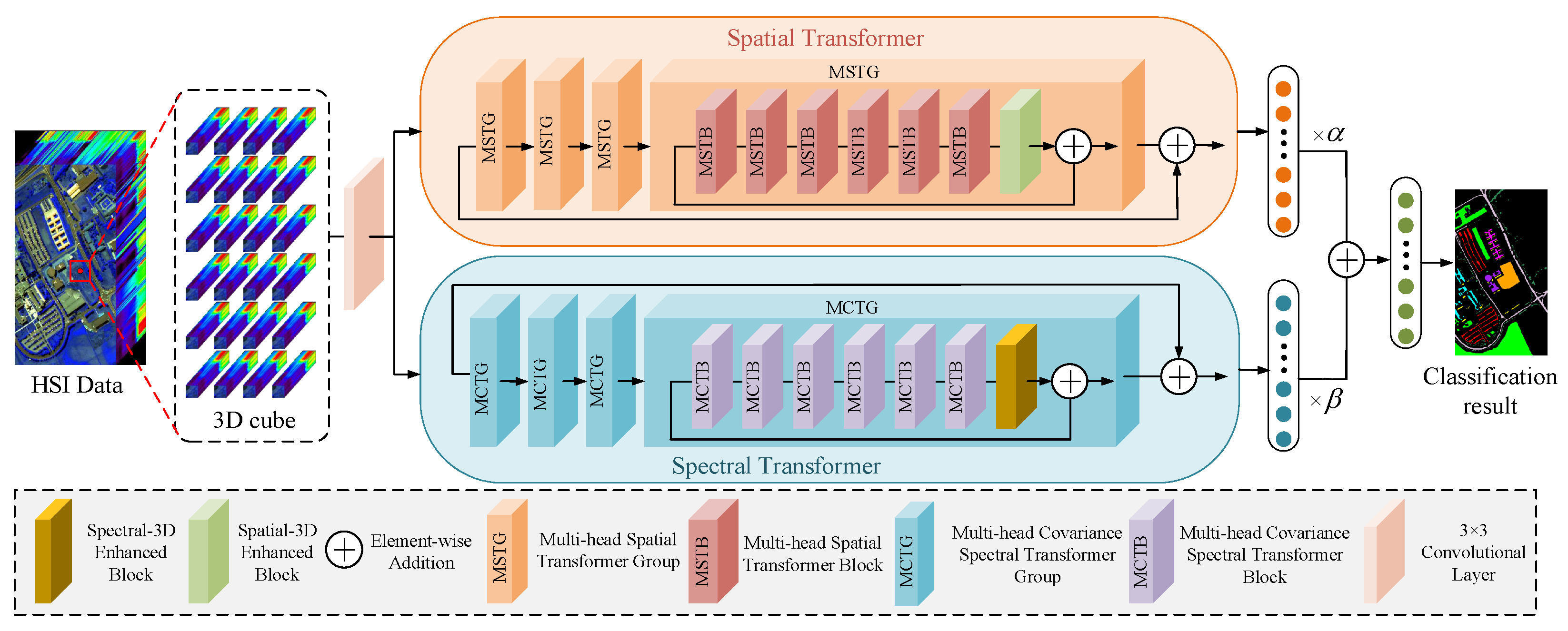
A parallel spectral–spatial transformer architecture is proposed for HSI classification, which is an efficient extraction of the spectral and spatial features in dual parallel branches.

2.

MCSA and MSSA, which are tailored for spectral and spatial feature extraction, improve the mining of local–global spatial and spectral sequence features.

3.

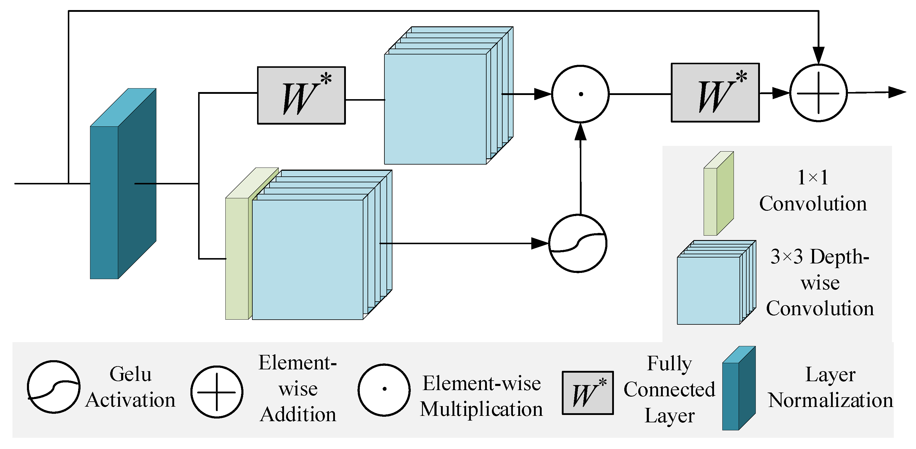
A local activation feed-forward network is proposed to enhance the extraction of local context signals by encoding information from spatially neighbouring pixel positions.

2. Methodology

As shown in Figure 1, our S2Former consists of a spatial transformer and a spectral transformer. In our S2Former, the 3D cube is taken as input. In other words, the target pixel and its adjacent pixels are fed into the network. Given a 3D cube $I\in {\mathbb{R}}^{M\times M\times O}$, where $M\times M$ denotes the spatial dimension, O is the number of bands. Our S2Former first applies a $3\times 3$ convolutional layer to obtain low-level feature embeddings $F_0\in {\mathbb{R}}^{M\times M\times C}$. Next, the shallow features $F_0$ are transported to the spatial transformer and spectral transformer in parallel. The shallow features $F_0$ are transformed into deep features $F_D^{Spa}\in {\mathbb{R}}^{M\times M\times C}$ and $F_D^{Spe}\in {\mathbb{R}}^{M\times M\times C}$. The spatial transformer contains multiple multi-head spatial transformer groups. Similarly, the spectral transformer consists of a series of multi-head spectral transformer groups. Then, we use the learnable weights $\alpha$ and $\beta$ to reweight the deep spatial features $F_D^{Spa}$ and the deep spectral features $F_D^{Spe}$.

The learnable weights $\alpha$ and $\beta$ optimise the spatial and spectral feature extraction by backward propagation. We obtain the output fused features $F_{out}\in {\mathbb{R}}^{M\times M\times C}$. Finally, the output fused features pass through the fully connected layer, mapping into predicted results.

2.1. Spatial Transformer

As illustrated in Figure 1, the spatial transformer is a stack of multi-head spatial transformer groups similar to the encoder to extract the deeper spatial features. The spatial transformer contains K multi-head spatial transformer groups (MSTG). The output spatial features extracted group by group are shown as

$$F_i^{Spa}=H_{MST{G}_i}\left(F_{i-1}^{Spa}\right),i=1,2,3,\cdots K,$$

(1)

where $H_{MST{G}_i}\left(·\right)$ is the i-th multi-head spatial transformer group. The multi-head spatial transformer group is a residual group with multiple multi-head spatial transformer blocks and a spatial-3D CNN block. Given the input feature $F_{i,0}^{Spa}$ of the i-th MSTG, we first extract intermediate spatial features $F_{i,j}^{Spa}$ by L multi-head spatial transformer blocks (MSTB) as

$$F_{i,j}^{Spa}=H_{MST{B}_{i,j}}\left(F_{i,j-1}^{Spa}\right),j=1,2,3,\cdots L,$$

(2)

where $H_{MST{B}_{i,j}}\left(·\right)$ denotes the j-th multi-head spatial transformer blocks in the i-th multi-head spatial transformer group. Next, the spatial features $F_{i,L}^{Spa}$ are enhanced by adding a spatial-3D enhanced block.

$$F_{i,out}^{Spa}=H_{Spa\_3D_i}\left(F_{i,L}^{Spa}\right),$$

(3)

where $H_{Spa\_3D_i}$ is the spatial-3D enhanced block in the i-th multi-head spatial transformer group. Next, we give a specific description of the multi-head spatial transformer block and spatial-3D enhanced block, which are the core components of the multi-head spatial transformer group.

2.1.1. Multi-Head Spatial Self-Attention

As shown in Figure 2b, a multi-head spatial transformer block contains a multi-head spatial self-attention (MSSA), a local activation feed-forward network (LAFN), and layer normalisation (LN) modules.

CNN-based methods exploit the local receptive field to extract features in HSI classification but have difficulty modeling pixels with long-range distanced positions. To capture non-local long-range dependencies, in our spatial transformer, we exploit MSSA to model long-range dependencies in spatial dimensions. As demonstrated in Figure 2, given an input $X_{in}\in {\mathbb{R}}^{M\times M\times C}$. MSSA aims to apply self-attention across global spatial locations and generates an attention map modeling the long-range dependencies and spatial interactions. $X_{in}$ is first linearly projected into $query$ $Q_{spa}\in {\mathbb{R}}^{M^2\times C}$, $key$ $K_{spa}\in {\mathbb{R}}^{M^2\times C}$ and $value$ $V_{spa}\in {\mathbb{R}}^{M^2\times C}$,

$$Q_{spa}=W^Q{X}_{in},K_{spa}=W^K{X}_{in},V_{spa}=W^V{X}_{in},$$

(4)

where $W^Q$, $W^K$, and $W^V$$\in {\mathbb{R}}^{C\times C}$ are learnable projection matrices. The attention matrix is thus computed by the self-attention mechanism. We apply dot-product interaction on $Q_{spa}$ and $K_{spa}$ to generate the spatial attention map $A_{spa}\in {\mathbb{R}}^{M^2\times M^2}$,

$$A_{spa}=Softmax\left(\frac{Q_{spa}·K_{spa}}{\sqrt{C}}+B\right),$$

(5)

$$Attention\left(Q_{spa},K_{spa},V_{spa}\right)=W_{out}·V_{spa}·A_{spa},$$

(6)

where $W_{out}\in {\mathbb{R}}^{C\times C}$ are also learnable projection matrices. B is the learnable relative positional encoding. Following multi-head SA [37], MSSA divides the number of channels into ‘heads’, then performs the attention function for ‘heads’ times in parallel and concatenates the results for multi-head results.

The LayerNorm (LN) layer is added before MSSA, and the residual connection is employed to obtain the output feature map ${\widehat{X}}_{in}^{Spa}\in {\mathbb{R}}^{M\times M\times C}$,

$${\widehat{X}}_{in}^{Spa}=H_{MSSA}\left(H_{LN}\left(X_{in}\right)\right)+X_{in},$$

(7)

where $H_{MSSA}(·)$ and $H_{LN}(·)$ denote the function of MSSA and the LayerNorm layer.

2.1.2. Local Activation Feed-Forward Network

In the traditional feed-forward network, the two fully connected layers are applied to expand the input feature channels and map the output channels back to the original input dimension. The fully connected layer processes token information point-wise in an identical manner. Thus, it neglects local information. In our work, we propose the local activation feed-forward network (LAFN), which aims at complementing local information by encoding information from spatially neighboring pixel positions. As shown in Figure 3, we complement the local details in the feed-forward network with two operations. First, we exploit the depth-wise convolution layer between the two fully connected layers to explore local signals from the global feature information in the regular branch. Second, we add a branch with depth-wise convolution to activate the local signal. The element-wise product is used to aggregate local and global information streams in two parallel branches.

Given an input feature ${\widehat{X}}_{in}\in {\mathbb{R}}^{M\times M\times C}$, LAFN is formulated as:

$$\begin{array}{cc}\hfill & X^{{}^{\prime }}=W_D\left(W^1\left(LN\left({\widehat{X}}_{in}\right)\right)\right)\odot H_{Gelu}\left(W_P{W}_{D}LN\left({\widehat{X}}_{in}\right)\right),\hfill \\ \hfill & X^{{}^{″}}={\widehat{X}}_{in}+W^2{X}^{{}^{\prime }},\hfill \end{array}$$

(8)

where $H_{Gelu}$ represents the Gelu non-linearity, and $W^{*}$ ( * denote 1 or 2) denote the fully connected layers. $W_P$ denotes point-wise convolution with a kernel size of $1\times 1$, and $W_D$ represents $3\times 3$ depth-wise convolution. Overall, the LAFN controls information flow through the activated local signal in our pipeline, thereby focusing on the fine details.

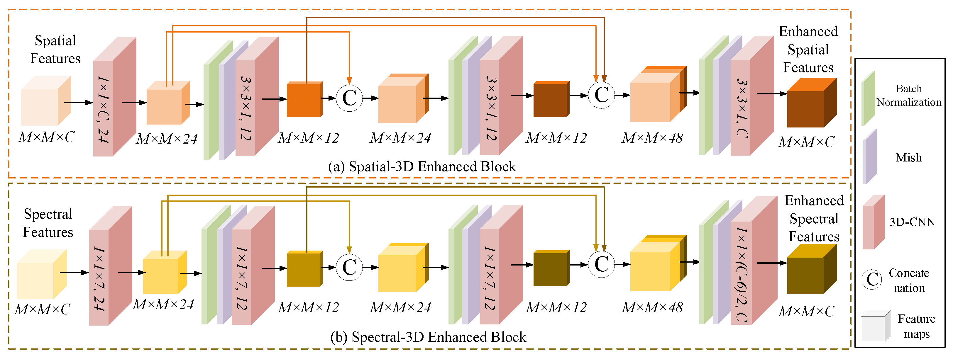
2.1.3. Spatial-3D Enhanced Block

The spatial-3D enhanced block is designed to maintain the global spatial feature and enhance the local spatial feature expression. As shown in Figure 4, we design the spatial-3D enhanced block similar to DBDA [30]. The input spatial feature $F_{i,L}^{Spa}\in {\mathbb{R}}^{M\times M\times C}$ is re-calibrated and reweighted through the remapping of local spatial feature coordinates with the spatial-3D enhanced block. First, the high-dimensional features across channels are mapped to low-dimensional ones by the $1\times 1\times C$ 3D convolution. Next, the features are transported to three spatial-3D enhanced layers with a dense connection. Each spatial-3D enhanced layer includes $3\times 3\times 1$ 3D convolution, 3D batch normalisation, and a Mish activation function.

2.2. Spectral Transformer

As exhibited in Figure 1, similar to the structure of the spatial transformer, the spectral transformer consists of K multi-head covariance spectral transformer groups (MCTG) that aim to extract the discriminative spectral features. The output spectral features extracted block by block are shown as

$$F_i^{Spe}=H_{MCT{G}_i}\left(F_{i-1}^{Spe}\right),i=1,2,3,\cdots K.$$

(9)

The multi-head covariance spectral transformer group is a residual group with multiple multi-head covariance spectral transformer blocks and a spectral-3D enhanced block. Given the input features $F_{i,0}^{Spe}$ of the i-th MCTG, we first extract intermediate spatial features $F_{i,j}^{Spe}$ by L multi-head covariance spectral transformer blocks (MCTB) as

$$F_{i,j}^{Spe}=H_{MCT{B}_{i,j}}\left(F_{i,j-1}^{Spe}\right),j=1,2,3,\cdots L,$$

(10)

where $H_{MCT{B}_{i,j}}(·)$ denotes the j-th multi-head spatial transformer blocks in the i-th multi-head covariance spectral transformer group. Next, the spatial features $F_{i,L}^{Spe}$ are enhanced by adding a spatial-3D CNN block,

$$F_{i,out}^{Spe}=H_{Spe\_3D_i}\left(F_{i,L}^{Spe}\right),$$

(11)

where $H_{Spe\_3D_i}(·)$ is the spectral-3D enhanced block in the i-th multi-head covariance spectral transformer group. Similarly, we elaborate the details of our multi-head covariance spectral transformer block and spectral-3D enhanced block.

2.2.1. Multi-Head Covariance Spectral Attention

Different from natural images, HSIs are also spectrally correlated and have numerous narrow bands. Capturing local and global spectral features are equally essential. In our work, we propose multi-head covariance spectral attention (MCSA) to model the inter-spectra similarity and long-range dependencies. Multi-head covariance spectral attention is intent on applying self-attention across spectral channels. MCSA computes cross-covariance across channels to generate an attention map encoding the global spectral signals. $X_{in}$ is first projected and reshaped into $query$ $Q_{spe}\in {\mathbb{R}}^{C\times M^2}$, $key$ $K_{spe}\in {\mathbb{R}}^{C\times M^2}$, and $value$ $V_{spe}\in {\mathbb{R}}^{C\times M^2}$ by applying $1\times 1$ point-wise convolutions $W_P$ followed by $3\times 3$ depth-wise convolutions $W_D$ to encode spatial context in a spectral-wise manner,

$$\begin{array}{cc}\hfill Q_{spe}=& W_P^Q{W}_D^Q{X}_{in},K_{spe}=W_P^K{W}_D^K{X}_{in},\hfill \\ \hfill & V_{spe}=W_P^V{W}_D^V{X}_{in}.\hfill \end{array}$$

(12)

Next, the spectral attention map is computed by the self-attention mechanism. We apply dot-product interaction on $Q_{spe}$ and $K_{spe}$ to generate the spectral attention map $A_{spe}\in {\mathbb{R}}^{C\times C}$,

$$A_{spe}=Softmax\left(\frac{Q_{spE}·K_{spE}}{\epsilon }+B\right),$$

(13)

$$Attention\left(Q_{spe},K_{spe},V_{spe}\right)=W_P·V_{spe}·A_{spe},$$

(14)

where $\epsilon$ is a learnable parameter to reweight the dot product of $Q_{spE}$ and $K_{spE}$ before applying the softmax function.

2.2.2. Spectral-3D Enhanced Block

The spectral-3D enhanced block is stacked behind L multi-head covariance spectral transformer blocks in each multi-head covariance spectral transformer group. The spectral-3D CNN block is designed to learn inter-spectra correlations after modeling the global spectral feature. Given the $F_{i,L}^{Spe}\in {\mathbb{R}}^{M\times M\times C}$, the spectral-3D enhanced block first applies a 3D convolution with the convolutional kernel of $1\times 1\times 7$ to obtain low-level local spectral features. Then, three spectral-3D enhanced layers are applied to extract spectral information. Each spectral-3D enhanced layer contains 3D convolution, 3D batch normalisation, and a Mish activation function. Except for the third 3D convolution layer, the remaining 3D convolution layers are with the convolutional kernel of $1\times 1\times 7$. The input of the i-th spectral-3D enhanced layer is the concatenated output of the former layers.

3. Experimental Results

To verify the performance of our S2Former, we conduct ablation studies and comparative experiments on four public datasets, including the Indian Pines dataset (IN), Pavia University dataset (UP), Botswana dataset (BS), and Houston dataset (HU). All experiments presented in this section are conducted on Nvidia GeForce RTX 3090 GPU.

3.1. Experimental Settings

Comparison Methods: To verify the effectiveness of the proposed S2Former, seven state-of-the-art HSI classifiers are used for comparison, including SVM [38], CDCNN [22], FDSSC [27], DBDA [30], SpectralFormer [34], HSI-Mixer [36], and BS2T [35].

Optimised Parameters: The proposed S2Former is trained on four datasets for 200 epochs. In addition, the batch size is 16, and the Adam optimiser with the 0.0005 learning rate was used to update the network parameters. For the compared methods and our S2Former, we select the input patches with a size of 9 × 9 × O. Training and test data of the four datasets are listed in

Table 1. Training and test data for each land cover category in the UP dataset.

Class	Category	Total Samples	Training	Test
1	Asphalt	6631	33	6598
2	Meadows	18,649	93	18,556
3	Gravel	2078	10	2068
4	Trees	3033	15	3018
5	Metal Sheets	1331	6	1325
6	Bare Soil	4978	25	4953
7	Bitumen	1316	6	1310
8	Bricks	3645	18	3627
9	Shadows	937	4	933
	Total	42,344	210	42,134

,

Table 2. Training and test data for each land cover category in the IN dataset.

Class	Category	Total Samples	Training	Test
1	Alfalfa	46	3	43
2	Corn-notill	1428	42	1386
3	Corn-mintill	830	24	806
4	Corn	237	7	230
5	Grass-pasture	483	14	469
6	Grass-trees	730	21	709
7	Grass-pasture-mowed	28	3	25
8	Hay-windrowed	478	14	464
9	Oats	20	3	17
10	Soybean-notill	972	29	943
11	Soybean-mintill	2455	73	2382
12	Soybean-clean	593	17	576
13	Wheat	205	6	199
14	Woods	1265	37	1228
15	Buildings-Grass-Trees-Drivers	386	11	375
16	Stone-Steel-Towers	93	3	90
	Total	10,249	307	9942

,

Table 3. Training and test data for each land cover category in the BS dataset.

Class	Category	Total Samples	Training	Test
1	Water	270	3	267
2	Hippo grass	101	2	99
3	Floodplain grasses1	251	3	248
4	Floodplain grasses2	215	3	212
5	Reeds1	269	3	266
6	Riparian	269	3	266
7	Fierscar2	259	3	256
8	Island interior	203	3	200
9	Acacia woodlands	314	3	311
10	Acacia shrublands	248	2	246
11	Acacia grasslands	305	3	302
12	Short mopane	181	2	179
13	Mixed mopane	268	3	265
14	Exposed soils	95	2	93
	Total	3248	42	3206

and

Table 4. Training and test data for each land cover category in the HU dataset.

Class	Category	Total Samples	Training	Test
1	Healthy Grass	1251	13	1238
2	Stressed Grass	1254	13	1241
3	Synthetic Grass	697	7	690
4	Tree	1244	12	1232
5	Soil	1252	13	1239
6	Water	325	3	322
7	Residential	1268	13	1255
8	Commercial	1244	12	1232
9	Road	1252	13	1239
10	Highway	1227	12	1215
11	Railway	1235	12	1223
12	Parking Lot 1	1234	12	1222
13	Parking Lot 2	469	5	464
14	Tennis Court	428	4	424
15	Running Track	660	7	653
	Total	15,011	151	14,860

. The UP dataset has the most significant number of samples, so only 0.5% of the training samples are selected, and the rest are used for testing. The labelled samples of each category in the IN dataset are unevenly distributed. To reasonably utilise the training samples, we choose 3% of the samples for training. For BS and HU, we use 1% labelled samples to train the models. A total of 99% labelled samples are used to test the performance of models.

Metrics: The classification performance is evaluated with overall accuracy (OA), average accuracy (AA), and kappa coefficient (Kappa) [39].

3.2. Ablation Studies

3.2.1. Discussion on Input Patch Size Comparison

Our S2Former is a 3D cube-wise-based HSI classification model. The size of the 3D cube determines the number of neighbouring pixels, which is the amount of information for the centre pixel. Therefore, the patch size is closely related to the performance of our S2Former. In order to explore the impact on HSI classification accuracy, we conduct an ablation study on the input HSI patch size. We exhibit the HSI classification results with the spatial dimension of the 3D cube ranging from 3 × 3 to 13 × 13 on four standard datasets. The quantitative results are shown in Figure 5. The patch size of the input 3D cube achieves a significant influence on classification performance. The patch size of $9\times 9$ obtains the optimal results for the four standard datasets.

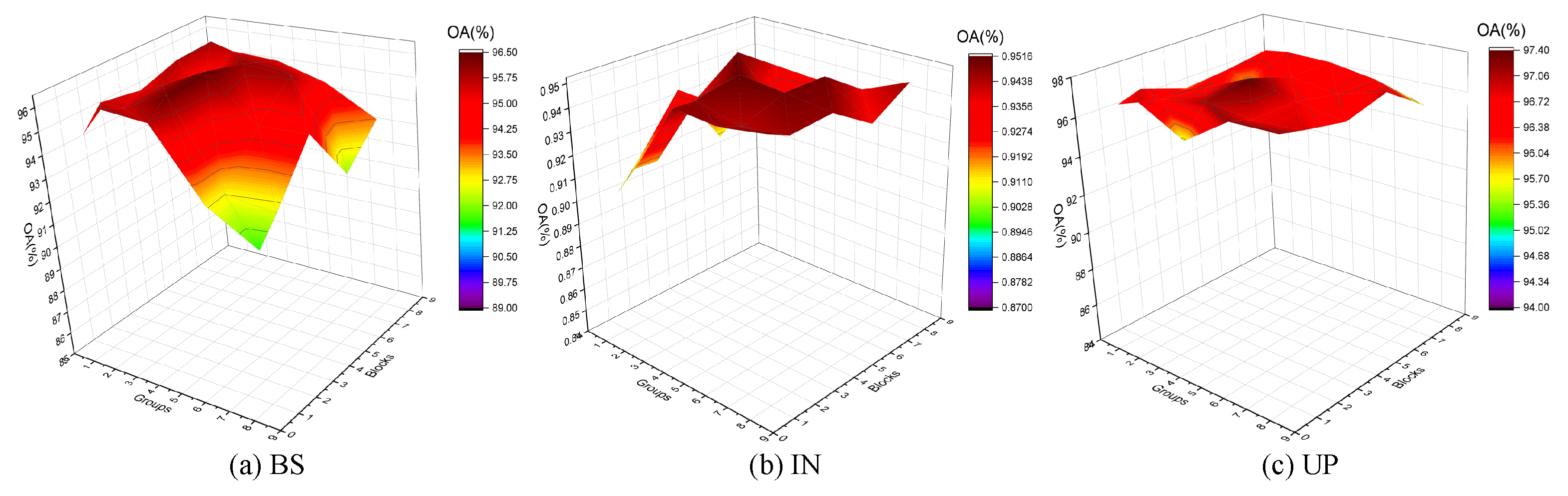
3.2.2. Discussion on Model Depth

The number of groups and blocks in the spatial transformer and spectral transformer represents the network depth of S2Former. We select the integer values of group and block in the range of $\left\{1,2,3,4,5,6,7,8\right\}$ and $\left\{1,2,3,4,5,6,7,8\right\}$, respectively. The classification performance (OA) of our S2Former different groups and blocks is shown in Figure 6. We show the effects of group number and block number on the Botswana dataset (in Figure 6a), Indian Pines dataset (in Figure 6b), and Pavia University dataset (in Figure 6c). It is observed that the OA is correlated with block number and group number. The blocks, including the multi-head spatial transformer block in the spatial transformer and the multi-head covariance spectral transformer block in the spectral transformer, are stacked as groups to capture the long-range dependency of HSI pixels and bands. However, the long-range dependency will be damaged when excessive blocks and groups are added. The group number and block number of our S2Former are set to 4 and 4 to find the desired results with reasonable computation efficiency.

3.2.3. Discussion on Parallel Spectral–Spatial Transformer Architecture

Our S2Former is a dual-stream architecture with a spectral transformer and spatial transformer in parallel, which is designed to capture the discriminative features in spectral and spatial dimensions. To demonstrate the effectiveness of dual-stream architecture, we compare the classification results among the single spatial transformer, single spectral transformer, and our S2Former. As shown in

Table 5. Break-down ablation study on proposed components.

	Spatial Transformer	Spectral Transformer		OA			AA			Kappa
(a)	MSSA+MLP	-	81.76	94.42	93.24	84.68	93.79	92.89	80.28	92.54	92.67
(b)	MSSA+LAFN	-	84.6	96.94	95.51	86.10	97.00	95.41	83.34	95.92	95.13
(c)	MSSA+MLP +Spatial-3D	-	83.53	96.40	95.10	86.41	96.47	95.12	82.18	95.21	94.69
(d)	MSSA+LAFN +Spatial-3D	-	84.93	97.21	95.89	86.57	97.07	95.77	83.36	96.30	95.54
(e)	-	MCSA+MLP	82.45	94.24	94.02	83.76	93.54	94.31	81.03	92.66	93.52
(f)	-	MCSA+LAFN	84.54	96.93	96.33	85.00	97.11	95.75	83.30	95.91	96.03
(g)	-	MCSA+MLP +Spectral-3D	84.25	96.39	95.19	84.26	96.54	94.99	82.99	95.19	94.79
(h)	-	MCSA+LAFN + Spectral -3D	84.81	97.08	96.19	86.10	97.41	96.13	83.34	96.27	96.01
S2Former	MSSA+LAFN Spatial-3D	MCSA+LAFN Spectral -3D	85.12	97.40	96.49	86.96	97.71	96.42	83.92	96.54	96.20

, we show the classification results of break-down ablation experiments on HU, UP, and BS datasets. The quantitative results of Table 5(d), (h), and S2Former demonstrate that the combination of the spectral transformer and spatial transformer achieves the optimal performance. Compared to our S2Former, the single spectral transformer or spatial transformer fails to capture the comprehensive spectral–spatial features.

3.2.4. Discussion on Self-Attention and Feed-Forward Network

The self-attention modules and feed-forward network used in the S2Former play a powerful role in classification performance. The proposed self-attention mechanisms, including MSSA in the spatial transformer and MCSA in the spectral transformer, aim to produce the global spatial and spectral features. Considering the weaknesses of traditional feed-forward networks, we design LAFN. To investigate the contribution of the proposed MSSA, MCSA, and LAFN, an ablation study is conducted. As seen in Table 5, it can be observed that our MCSA shows a comparable ability of feature extraction compared to MSSA. The spectral feature representation is equally important for HSI classification with a redundant spectrum. Table 5(b) and (f) confirm that LAFN obtains a significant gain compared to a traditional MLP. It can be attributed to a supplement of the local details.

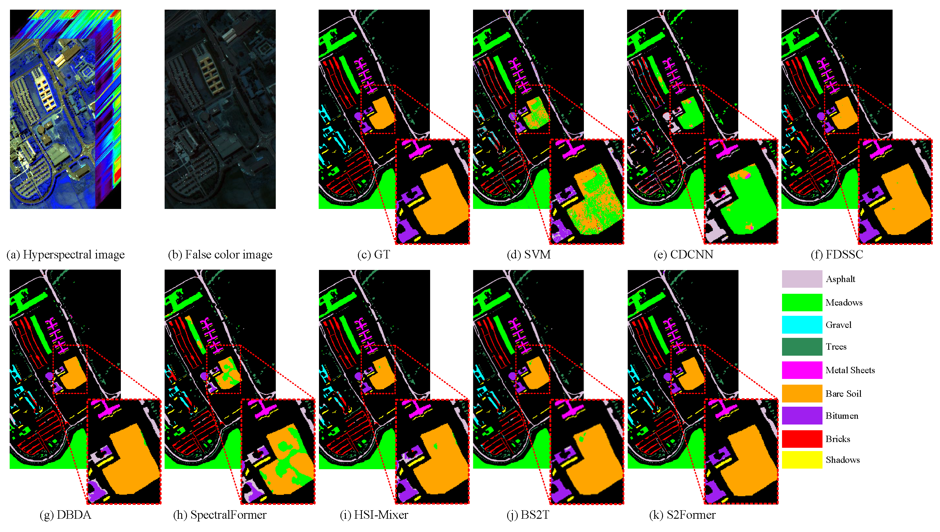
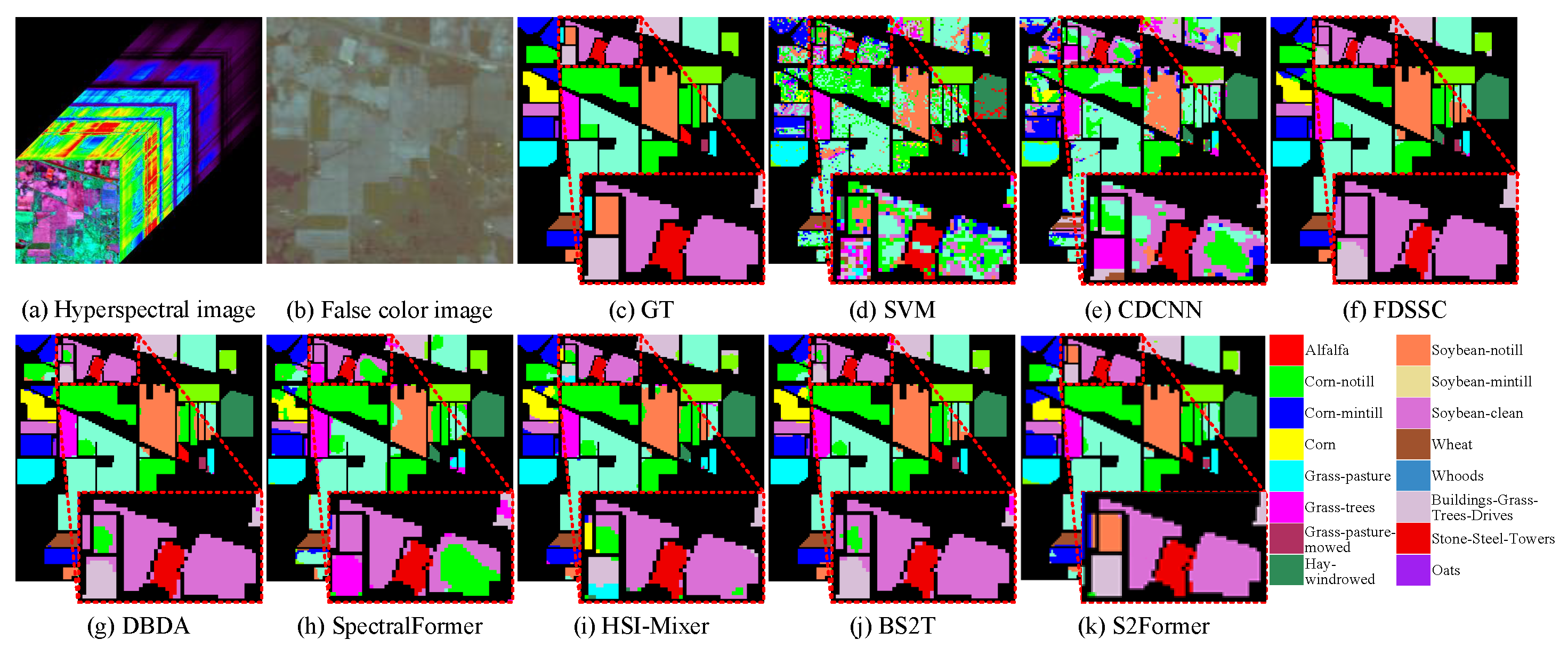
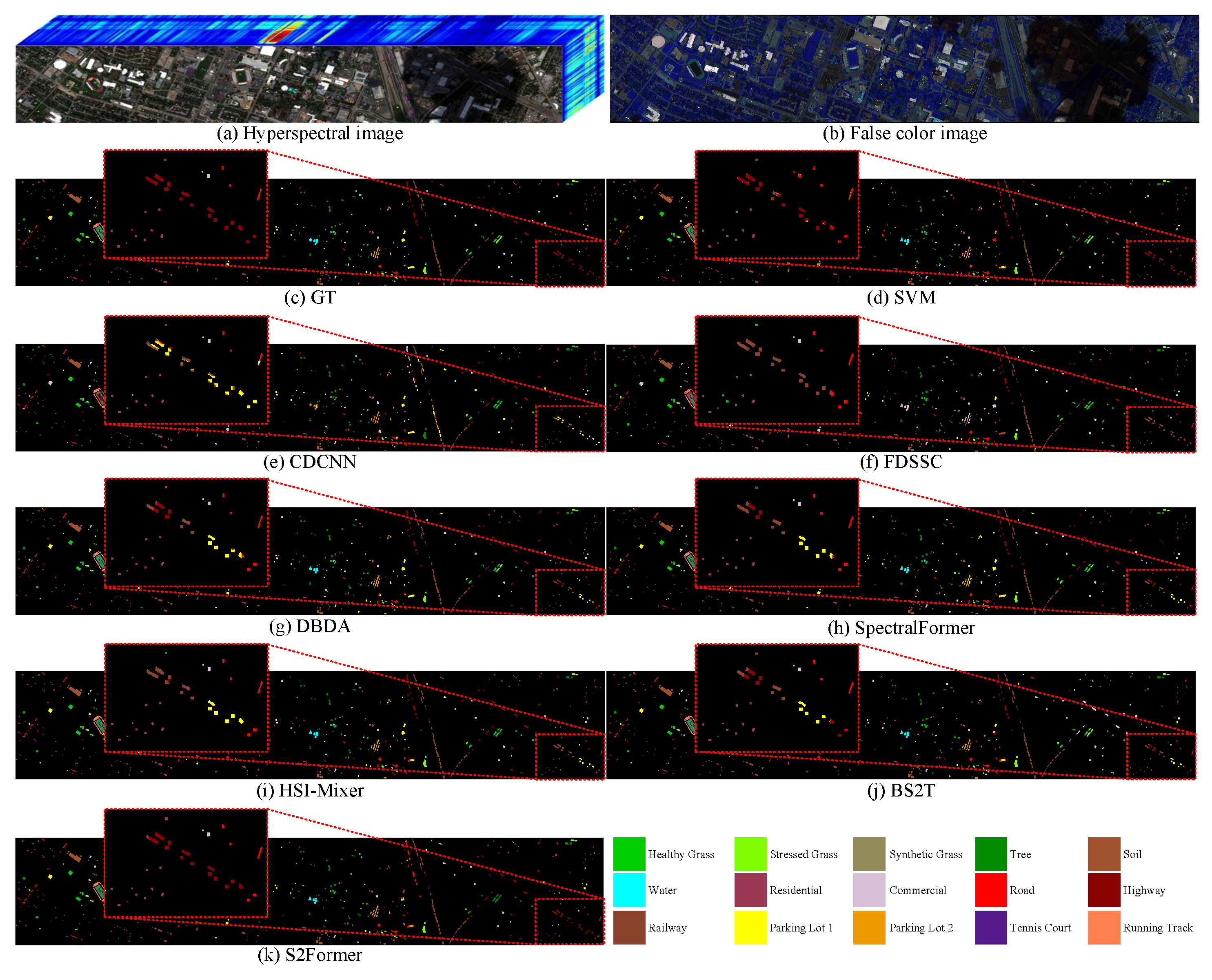
3.3. Comparison with Other Methods

To confirm the superiority of our S2Former, seven state-of-the-art classifiers are used for comparison. Except for SVM, the remaining six methods are patch-based HSI classifiers. Furthermore, the compared classifiers and our S2Former maintain the same parameter settings.

The quantitative results are shown in

Table 6. Comparison of quantitative results on the UP dataset.

Class	SVM	CDCNN	FDSSC	DBDA	Spectral Former	HSI-Mixer	BS2T	S2Former
1	83.87	80.60	87.22	94.15	85.97	92.77	93.93	94.77
2	86.33	93.10	99.50	99.01	96.26	97.10	98.64	98.16
3	67.75	62.45	72.42	95.06	92.43	93.70	97.90	98.02
4	96.89	98.76	97.11	97.76	97.71	98.66	98.36	99.06
5	94.28	99.45	99.01	99.34	99.23	98.35	98.61	100.00
6	84.55	86.04	97.83	98.11	94.48	97.32	98.55	98.99
7	66.46	73.84	69.78	99.68	89.36	96.56	99.20	98.80
8	70.70	72.71	82.76	86.61	77.95	87.03	84.39	91.55
9	99.89	98.32	99.55	98.47	97.90	98.95	98.83	100.00
OA(%)	83.99	87.48	94.30	96.56	92.43	96.48	96.97	97.40
AA(%)	83.41	85.03	89.46	96.47	92.37	95.60	96.69	97.71
Kappa(%)	78.24	83.20	92.41	95.43	89.84	95.31	95.92	96.54

,

Table 7. Comparison of quantitative results on the IN dataset.

Class	SVM	CDCNN	FDSSC	DBDA	Spectral Former	HSI-Mixer	BS2T	S2Former
1	24.20	90.39	89.55	99.76	69.23	99.67	100.00	100.00
2	55.98	74.08	95.02	95.10	83.63	89.43	93.50	95.48
3	64.45	60.55	93.05	94.53	84.21	80.86	93.94	89.28
4	43.19	86.67	96.75	95.23	96.33	93.76	95.78	98.70
5	84.59	88.08	97.63	95.23	96.62	95.43	98.62	98.34
6	82.11	86.31	97.34	97.84	88.36	92.94	97.93	99.70
7	58.75	87.08	80.78	73.47	63.98	86.82	76.89	100.00
8	87.87	86.51	98.41	100.00	88.12	89.51	99.98	100.00
9	46.58	71.92	58.33	96.54	74.37	91.58	94.43	100.00
10	65.10	83.29	91.48	89.57	83.27	89.01	88.00	94.82
11	63.11	72.24	93.08	94.23	80.52	95.21	96.10	97.21
12	49.67	69.71	90.21	91.85	84.57	82.56	90.94	99.42
13	88.59	96.55	99.58	98.92	92.47	98.76	98.39	100.00
14	89.89	90.37	97.85	97.89	91.97	94.14	96.10	97.90
15	61.63	75.65	93.40	95.57	89.87	89.43	94.84	91.22
16	99.23	91.30	98.80	96.95	89.87	95.69	96.69	78.76
OA(%)	69.06	78.24	92.35	94.89	85.46	92.50	94.94	95.16
AA(%)	66.56	81.92	91.95	94.80	84.79	91.55	94.51	96.30
Kappa(%)	64.28	74.94	91.25	94.17	83.29	91.44	94.73	94.47

,

Table 8. Comparison of quantitative results on the BS dataset.

Class	SVM	CDCNN	FDSSC	DBDA	Spectral Former	HSI-Mixer	BS2T	S2Former
1	90.38	89.29	97.21	98.56	89.76	96.02	93.92	98.74
2	34.58	74.72	87.97	93.38	56.31	83.03	82.76	86.48
3	86.71	68.45	99.54	99.27	83.01	100.00	100.00	100.00
4	56.73	57.03	84.71	89.87	83.99	87.93	94.60	97.99
5	87.27	81.65	94.07	94.28	90.21	90.82	92.38	81.72
6	56.63	59.85	82.08	92.01	70.31	90.41	94.90	97.80
7	89.09	89.39	98.54	97.84	99.53	99.39	100.00	100.00
8	76.91	69.52	96.99	99.20	96.77	99.45	97.04	98.00
9	75.78	74.52	88.85	96.09	96.49	90.55	96.94	98.02
10	87.69	75.26	91.42	91.35	93.33	93.07	74.08	94.42
11	82.25	95.84	97.57	98.61	83.06	97.67	100.00	100.00
12	60.38	89.73	99.72	99.89	86.26	97.78	99.44	96.72
13	91.06	71.00	93.01	96.86	89.88	99.39	100.00	100.00
14	79.91	91.09	98.18	97.67	99.55	99.29	100.00	100.00
OA(%)	73.15	74.89	91.94	95.47	83.42	94.11	94.34	96.49
AA(%)	75.38	77.67	93.56	96.06	87.03	94.63	94.71	96.42
Kappa(%)	71.03	72.85	91.27	95.09	82.08	93.62	93.87	96.20

and

Table 9. Comparison of quantitative results on the HU dataset.

Class	SVM	CDCNN	FDSSC	DBDA	Spectral Former	HSI-Mixer	BS2T	S2Former
1	69.46	92.73	79.90	83.77	77.60	83.97	94.19	85.92
2	93.52	93.20	95.09	93.75	88.60	93.22	94.13	95.38
3	61.67	96.62	99.15	96.66	96.00	100.00	100.00	100.00
4	91.26	98.57	94.90	93.85	92.59	97.33	85.64	98.82
5	80.70	93.72	93.81	94.75	90.75	94.33	88.44	96.08
6	94.08	100.00	90.00	92.26	97.27	97.75	100.00	100.00
7	65.85	73.68	72.55	83.14	78.23	79.01	80.58	84.16
8	57.54	66.31	72.30	92.44	85.19	93.08	88.99	85.32
9	75.37	65.18	73.16	75.81	69.60	71.34	70.05	76.64
10	66.04	69.31	74.23	72.73	64.94	64.88	68.89	74.44
11	61.10	61.46	69.28	80.09	69.27	71.29	63.11	80.60
12	67.74	63.82	76.41	71.64	63.52	72.64	65.79	71.20
13	97.02	26.30	49.08	89.70	73.16	90.51	65.98	74.82
14	83.87	93.19	98.23	90.51	95.32	95.10	97.22	92.92
15	65.75	98.86	96.80	89.48	92.78	95.58	95.74	86.82
OA(%)	71.92	78.75	80.62	83.95	79.07	82.70	81.78	85.12
AA(%)	75.40	79.53	82.33	86.69	82.32	86.67	83.92	86.96
Kappa(%)	69.58	76.99	79.00	82.63	77.35	81.28	80.30	83.92

, which represent the detailed classification results of the UP, IN, BS, and HU datasets, respectively. Obviously, our S2Former achieves more significant results than the other seven classifiers. In Table 6, the proposed method achieves 97.40% in OA, 97.60% in AA, and 96.54% in Kappa. SVM achieves the worst results. For the 2D-CNN-based CDCNN, the classification accuracy is only better than SVM. FDSSC exploits the dense connection to improve the network performance. DBDA extracts spatial and spectral features by adding attention mechanisms and obtains superior classification accuracy. BS2T, which also employs the transformer architecture, obtains the performance second only to our method.

In addition, in Table 6, Table 7, Table 8 and Table 9, the best classification accuracy for each land cover category is shown in bold. Our S2Former also achieves satisfactory results in each land cover category. Although the seventh land cover category Grass-pasture-mowed in Table 7 only has three training samples, the classification accuracy of S2Former is improved by 13.18% compared to the second-accuracy HSI-Mixer. S2Former uses the proposed self-attention mechanisms to simulate global spatial–spectral features and extract the discriminative features at a maximum extent. Therefore, the proposed S2Former achieves a significant gain in fine-grained classification.

In Table 7, the tenth (Soybean-no-till), eleventh (Soybean-min-till), and twelfth (Soybean-clean) land cover categories in the IN dataset have very similar characteristics. S2Former obtains the highest classification accuracy (94.82%, 97.21%, and 99.42%) than other SOTA methods. Similar situations can also be found in the BS dataset and HU dataset, such as Acacia woodlands, Acacia shrublands, and Acacia grasslands in Table 8, and Stressed Grass and Synthetic Grass in Table 9. Our proposed S2Former obtains outstanding classification results in four datasets.

To visually demonstrate the performance of our S2Former, we present the false-color images, the Ground Truth maps, and the classification maps for each method in Figure 7, Figure 8, Figure 9 and Figure 10. Our method has clearer boundaries and less noise and outperforms the other seven SOTA methods, which benefits from the dual-stream spectral–spatial transformer structure in S2Former. SVM performs the worst among all methods, with large intraclass noise. CDCNN, with a simple network structure, also has a lot of noise. Although the other five comparison methods achieve relatively accurate and smooth classification maps, they still have some errors compared with the proposed S2Former.

Specifically, in Figure 7, CDCNN misclassifies Bare Soil into Meadows, resulting in poor classification results. Although DBDA works better in the Bare Soil class, it has obvious misclassification in the Bitumen class. Since our S2Former extracts global features and supplements local details, the classification results are slightly better than BS2T in the visualisation results. In Figure 8, compared methods have misclassified two similar land cover categories (Soybean-notill and Soybean-clean). We propose multi-head covariance spectral attention in the spectral transformer branch to explore highly similarity and correlation across the spectral dimension. Therefore, our S2Former can accurately classify these two land cover categories. Considering the messy distribution of labelled pixels in the BS and HU datasets, we perform local magnification on a specific area of the two datasets to exhibit the performance. As shown in Figure 9 and Figure 10, when dealing with isolated objects of small size, other methods maintain an over-smoothing phenomenon or misclassification occurs. Our method maintains appreciable classification results even in cluttered pixels.

3.4. Comparison of the Complexity

We have compared the complexity of our S2Former and state-of-the-art HSI classification algorithms in terms of time and space consumption. We select Flops and params to represent space consumption and Training time to represent time consumption.

Table 10. Comparison of the complexity of time-space consumption.

	CDCNN	FDSSC	DBDA	Spectral Former	HSI-Mixer	BS2T	S2Former
Training time (s)	498.97	1459.14	1229.35	1307.76	1752.50	1549.89	1855.85
Flops (G)	2.60	22.71	13.82	13.25	12.57	13.84	12.76
params (M)	2.91	1.23	0.38	0.51	0.25	0.38	0.54

shows the number of parameters and Flops and the training times. The results demonstrate that our S2Former achieves higher performance and has a better tradeoff between model size and performance. Our S2Former achieves significant PSNR gains at the cost of less model complexity increase.

4. Conclusions

In this article, we propose a novel spectral–spatial transformer (S2Former) for HSI classification. S2Former exploits the dual-branch transformer architecture to extract discriminative feature streams with the local and global receptive fields in the spatial and spectral dimensions. First, the spatial transformer consists of two components: the proposed MSSA applied self-attention in the spatial dimension to encode the long-term spatial position information, and the spatial-3D enhanced block adaptive captures the local spatial information. Similarly, the spectral transformer exploits MCSA to compute covariance-based channel maps in modeling the long-range spectrum dependence. The spectral-3D enhanced block is introduced to learn the subtle spectral discrepancies. LAFN is designed to replace traditional MLP in the transformer block, which activates the global features and complements local details. Finally, the spatial and spectral features extracted from the dual branches are used to obtain the classification result.

Extensive experimental results demonstrate the superiority of our S2Former over SOTA HSI classifiers. Our S2Former has good scalability in spectral–spatial feature extraction for other HSI tasks.

References

1. Chen, F.; Jiang, H.; Van de Voorde, T.; Lu, S.; Xu, W.; Zhou, Y. Land cover mapping in urban environments using hyperspectral APEX data: A study case in Baden, Switzerland. Int. J. Appl. Earth Obs. Geoinf. 2018, 71, 70–82. [Google Scholar] [CrossRef]
2. Sethy, P.K.; Pandey, C.; Sahu, Y.K.; Behera, S.K. Hyperspectral imagery applications for precision agriculture-a systemic survey. Multimed. Tools Appl. 2021, 81, 3005–3038. [Google Scholar] [CrossRef]
3. Zhao, X.; Niu, J.; Liu, C.; Ding, Y.; Hong, D. Hyperspectral Image Classification Based on Graph Transformer Network and Graph Attention Mechanism. IEEE Geosci. Remote Sens. Lett. 2022, 19, 1–5. [Google Scholar] [CrossRef]
4. Pour, A.B.; Zoheir, B.; Pradhan, B.; Hashim, M. Editorial for the special issue: Multispectral and hyperspectral remote sensing data for mineral exploration and environmental monitoring of mined areas. Remote Sens. 2021, 13, 519. [Google Scholar] [CrossRef]
5. Peyghambari, S.; Zhang, Y. Hyperspectral remote sensing in lithological mapping, mineral exploration, and environmental geology: An updated review. J. Appl. Remote Sens. 2021, 15, 031501. [Google Scholar] [CrossRef]
6. Cao, X.; Fu, X.; Xu, C.; Meng, D. Deep spatial-spectral global reasoning network for hyperspectral image denoising. IEEE Trans. Geosci. Remote Sens. 2021, 60, 1–14. [Google Scholar] [CrossRef]
7. Zhang, H.; Cai, J.; He, W.; Shen, H.; Zhang, L. Double low-rank matrix decomposition for hyperspectral image denoising and destriping. IEEE Trans. Geosci. Remote Sens. 2021, 60, 1–19. [Google Scholar] [CrossRef]
8. Rasti, B.; Koirala, B. SUnCNN: Sparse unmixing using unsupervised convolutional neural network. IEEE Geosci. Remote Sens. Lett. 2021, 19, 1–5. [Google Scholar] [CrossRef]
9. Zhang, X.; Sun, Y.; Zhang, J.; Wu, P.; Jiao, L. Hyperspectral unmixing via deep convolutional neural networks. IEEE Geosci. Remote Sens. Lett. 2018, 15, 1755–1759. [Google Scholar] [CrossRef]
10. He, J.; Yuan, Q.; Li, J.; Xiao, Y.; Liu, X.; Zou, Y. DsTer: A dense spectral transformer for remote sensing spectral super-resolution. Int. J. Appl. Earth Obs. Geoinf. 2022, 109, 102773. [Google Scholar] [CrossRef]
11. Li, Q.; Wang, Q.; Li, X. Exploring the Relationship Between 2D/3D Convolution for Hyperspectral Image Super-Resolution. IEEE Trans. Geosci. Remote Sens. 2021, 59, 8693–8703. [Google Scholar] [CrossRef]
12. Zou, C.; Zhang, C. Hyperspectral image super-resolution using cluster-based deep convolutional networks. Signal Process. Image Commun. 2023, 110, 116884. [Google Scholar] [CrossRef]
13. Zou, C.; Huang, X. Hyperspectral image super-resolution combining with deep learning and spectral unmixing. Signal Process. Image Commun. 2020, 84, 115833. [Google Scholar] [CrossRef]
14. Xie, W.; Zhang, X.; Li, Y.; Wang, K.; Du, Q. Background learning based on target suppression constraint for hyperspectral target detection. IEEE J. Sel. Top. Appl. Earth Obs. Remote Sens. 2020, 13, 5887–5897. [Google Scholar] [CrossRef]
15. Zhao, X.; Hou, Z.; Wu, X.; Li, W.; Ma, P.; Tao, R. Hyperspectral target detection based on transform domain adaptive constrained energy minimization. Int. J. Appl. Earth Obs. Geoinf. 2021, 103, 102461. [Google Scholar] [CrossRef]
16. Qu, J.; Xu, Y.; Dong, W.; Li, Y.; Du, Q. Dual-Branch Difference Amplification Graph Convolutional Network for Hyperspectral Image Change Detection. IEEE Trans. Geosci. Remote Sens. 2022, 60, 1–12. [Google Scholar] [CrossRef]
17. Sun, G.; Zhang, X.; Jia, X.; Ren, J.; Zhang, A.; Yao, Y.; Zhao, H. Deep fusion of localized spectral features and multi-scale spatial features for effective classification of hyperspectral images. Int. J. Appl. Earth Obs. Geoinf. 2020, 91, 102157. [Google Scholar] [CrossRef]
18. Yu, D.; Li, Q.; Wang, X.; Xu, C.; Zhou, Y. A Cross-Level Spectral—Spatial Joint Encode Learning Framework for Imbalanced Hyperspectral Image Classification. IEEE Trans. Geosci. Remote Sens. 2022, 60, 1–17. [Google Scholar] [CrossRef]
19. Kumar, V.; Singh, R.S.; Dua, Y. Morphologically dilated convolutional neural network for hyperspectral image classification. Signal Process. Image Commun. 2022, 101, 116549. [Google Scholar] [CrossRef]
20. Mookambiga, A.; Gomathi, V. Kernel eigenmaps based multiscale sparse model for hyperspectral image classification. Signal Process. Image Commun. 2021, 99, 116416. [Google Scholar] [CrossRef]
21. Ghasrodashti, E.K.; Sharma, N. Hyperspectral image classification using an extended Auto-Encoder method. Signal Process. Image Commun. 2021, 92, 116111. [Google Scholar] [CrossRef]
22. Lee, H.; Kwon, H. Contextual deep CNN based hyperspectral classification. In Proceedings of the 2016 IEEE International Geoscience and Remote Sensing Symposium (IGARSS), Beijing, China, 10–15 July 2016; IEEE: Piscataway, NJ, USA, 2016; pp. 3322–3325. [Google Scholar]
23. Chen, Y.; Jiang, H.; Li, C.; Jia, X.; Ghamisi, P. Deep feature extraction and classification of hyperspectral images based on convolutional neural networks. IEEE Trans. Geosci. Remote Sens. 2016, 54, 6232–6251. [Google Scholar] [CrossRef]
24. He, K.; Zhang, X.; Ren, S.; Sun, J. Deep residual learning for image recognition. In Proceedings of the IEEE Conference on Computer Vision and Pattern Recognition, Las Vegas, NV, USA, 27–30 June 2016; pp. 770–778. [Google Scholar]
25. Huang, G.; Liu, Z.; Van Der Maaten, L.; Weinberger, K.Q. Densely connected convolutional networks. In Proceedings of the IEEE Conference on Computer Vision and Pattern Recognition, Honolulu, HI, USA, 21–26 July 2017; pp. 4700–4708. [Google Scholar]
26. Zhong, Z.; Li, J.; Luo, Z.; Chapman, M. Spectral–spatial residual network for hyperspectral image classification: A 3-D deep learning framework. IEEE Trans. Geosci. Remote Sens. 2017, 56, 847–858. [Google Scholar] [CrossRef]
27. Wang, W.; Dou, S.; Jiang, Z.; Sun, L. A fast dense spectral–spatial convolution network framework for hyperspectral images classification. Remote Sens. 2018, 10, 1068. [Google Scholar] [CrossRef]
28. Fang, B.; Li, Y.; Zhang, H.; Chan, J.C.W. Hyperspectral images classification based on dense convolutional networks with spectral-wise attention mechanism. Remote Sens. 2019, 11, 159. [Google Scholar] [CrossRef]
29. Ma, W.; Yang, Q.; Wu, Y.; Zhao, W.; Zhang, X. Double-branch multi-attention mechanism network for hyperspectral image classification. Remote Sens. 2019, 11, 1307. [Google Scholar] [CrossRef]
30. Li, R.; Zheng, S.; Duan, C.; Yang, Y.; Wang, X. Classification of hyperspectral image based on double-branch dual-attention mechanism network. Remote Sens. 2020, 12, 582. [Google Scholar] [CrossRef]
31. Dosovitskiy, A.; Beyer, L.; Kolesnikov, A.; Weissenborn, D.; Zhai, X.; Unterthiner, T.; Dehghani, M.; Minderer, M.; Heigold, G.; Gelly, S.; et al. An image is worth 16 × 16 words: Transformers for image recognition at scale. arXiv 2020, arXiv:2010.11929. [Google Scholar]
32. Xue, Z.; Tan, X.; Yu, X.; Liu, B.; Yu, A.; Zhang, P. Deep Hierarchical Vision Transformer for Hyperspectral and LiDAR Data Classification. IEEE Trans. Image Process. 2022, 31, 3095–3110. [Google Scholar] [CrossRef]
33. Zhao, Z.; Hu, D.; Wang, H.; Yu, X. Convolutional Transformer Network for Hyperspectral Image Classification. IEEE Geosci. Remote Sens. Lett. 2022, 19, 1–5. [Google Scholar] [CrossRef]
34. Hong, D.; Han, Z.; Yao, J.; Gao, L.; Zhang, B.; Plaza, A.; Chanussot, J. SpectralFormer: Rethinking hyperspectral image classification with transformers. IEEE Trans. Geosci. Remote Sens. 2021, 60, 1–15. [Google Scholar] [CrossRef]
35. Song, R.; Feng, Y.; Cheng, W.; Mu, Z.; Wang, X. BS2T: Bottleneck Spatial–Spectral Transformer for Hyperspectral Image Classification. IEEE Trans. Geosci. Remote Sens. 2022, 60, 1–17. [Google Scholar] [CrossRef]
36. Liang, H.; Bao, W.; Shen, X.; Zhang, X. HSI-mixer: Hyperspectral image classification using the spectral–spatial mixer representation from convolutions. IEEE Geosci. Remote Sens. Lett. 2022, 19, 1–5. [Google Scholar] [CrossRef]
37. Vaswani, A.; Shazeer, N.; Parmar, N.; Uszkoreit, J.; Jones, L.; Gomez, A.N.; Kaiser, L.U.; Polosukhin, I. Attention is All you Need. In Advances in Neural Information Processing Systems; Curran Associates, Inc.: Nice, France, 2017; Volume 30. [Google Scholar]
38. Melgani, F.; Bruzzone, L. Classification of hyperspectral remote sensing images with support vector machines. IEEE Trans. Geosci. Remote Sens. 2004, 42, 1778–1790. [Google Scholar] [CrossRef]
39. Gao, H.; Chen, Z.; Xu, F. Adaptive spectral-spatial feature fusion network for hyperspectral image classification using limited training samples. Int. J. Appl. Earth Obs. Geoinf. 2022, 107, 102687. [Google Scholar] [CrossRef]
Figure 1. The network architecture of our S2Former. S2Former adopts the parallel spatial transformer and spectral transformer to individually explore discriminative features in spatial and spectral dimensions. The transformer branches mainly consist of residual in residual design, incorporating a multi-head spatial transformer block and multi-head covariance spectral transformer block.
Electronics 12 03937 g001
Figure 2. Illustration of the multi-head spatial transformer block (MSTB) and multi-head covariance spectral transformer block (MCTB). The core modules of (a) MCTB and (b) MSTB are (c) multi-head covariance spectral attention, (d) multi-head spatial self-attention, and the local activation feed-forward network.
Electronics 12 03937 g002
Figure 3. The architecture of the local activation feed-forward network (LAFN). LAFN exploits depth-wise convolution and the fully connected layer to encode local signals and global information.
Electronics 12 03937 g003
Figure 4. The detailed schematic of the spatial-3D enhanced block and spectral-3D enhanced block.
Electronics 12 03937 g004
Figure 5. Model performance comparison under different input patch sizes.
Electronics 12 03937 g005
Figure 6. The quantitative results in terms of OA with different model depths.
Electronics 12 03937 g006
Figure 7. Qualitative comparison results for the UP dataset. (a) Hyperspectral image. (b) False color image. (c) GT. (d) SVM. (e) CDCNN. (f) FDSSC. (g) DBDA. (h) SpectralFormer. (i) HSI-Mixer. (j) BS2T. (k) S2Former.
Electronics 12 03937 g007
Figure 8. Comparison of qualitative results for the IN dataset. (a) Hyperspectral image. (b) False color image. (c) GT. (d) SVM. (e) CDCNN. (f) FDSSC. (g) DBDA. (h) SpectralFormer. (i) HSI-Mixer. (j) BS2T. (k) S2Former.
Electronics 12 03937 g008
Figure 9. Comparison of qualitative results for the BS dataset. (a) Hyperspectral image. (b) False color image. (c) GT. (d) SVM. (e) CDCNN. (f) FDSSC. (g) DBDA. (h) SpectralFormer. (i) HSI-Mixer. (j) BS2T. (k) S2Former.
Electronics 12 03937 g009
Figure 10. Comparison of qualitative results for the HU dataset. (a) Hyperspectral image. (b) False color image. (c) GT. (d) SVM. (e) CDCNN. (f) FDSSC. (g) DBDA. (h) SpectralFormer. (i) HSI-Mixer. (j) BS2T. (k) S2Former.
Electronics 12 03937 g010