Ship Diesel Engine Fault Diagnosis Using Data Science and Machine Learning

Abstract

One of the most important elements of the reliability structure of a motor vessel is its power subsystem, with the most crucial component being the engine. An engine failure excludes the ship from operation or significantly limits its operation. Therefore, accurate fault diagnosis should be a crucial issue for modern maintenance strategies. In mechanical engineering, the vibration and acoustic signals recorded during the operation of the device are the most meaningful data used to identify the reliability state. In this paper, a novel system-oriented method of reliability state identification is proposed. The method consists of the analysis of the vibration and noise signals collected on each of the engine cylinders using supervised machine learning. The main novelty of this method is data augmentation application and SVM classifier implementation. Due to these aspects, the method becomes robust in the case of poor-quality data or a limited and incomplete learning dataset. The quality of the proposed identification method was evaluated by addressing a new industrial issue (Sulzer 6AL20/24 marine engine reliability state identification). During the tests, the efficiency of the method was analyzed in the case of a complete learning data set (all types of inability states were presented in the learning data set) and an incomplete learning data set (in the testing data set, there were new types of inability states). As a result, in both cases, a very high (100%) identification accuracy of the reliability state and the type of inability state was obtained. This is a significant increase in accuracy (4.6% for the complete and 22% for the incomplete learning data set) in comparison to the efficiency of the same method without the use of machine learning and data science.

1. Introduction

A motor vessel during operation can be considered an isolated technical system, which must independently cover all of its power demands. The power is produced by the ship’s engines—very often diesel engines. The crucial element of the reliability structure of the vessel power system is the engine (or the cylinders of the engine) [1]; therefore, its technical condition should be the subject of continuous diagnostics.

In order to decrease the engine fault risk and to shorten the period in which the engine is out of order, it is necessary to identify its operation condition online and to classify the type of operation disturbance before the engine is stopped and service activities begin. Additionally, abnormalities in the operation of engine fuel installation elements can increase carbon emissions, which should be avoided, considering that the shipping industry has always been an important contributor to global carbon emissions, accounting for approximately 3.1% of the total [2]. Therefore, the main objective of the present research was the identification of the operating condition of the ship engine and the type of failure experienced when the inability state occurs. Because the object of the research was a crucial technical system whose failure is a source of high costs or poses a threat to human life, the research focused on well known, industrially tested, and robust methods that allow for a high level of identification accuracy.

Some of the most meaningful diagnostic signals for rotating mechanical devices are vibration and noise signals [3]. Therefore, in the present work, the task of identifying the reliability state and the type of inability state (the fault diagnosis) of the research object was performed by analyzing the vibration and noise signals recorded during operation.

The analysis of the vibration and noise signals can be performed in the frequency or time domain. In the frequency domain, in order to determine fault frequencies, the Fourier [4,5] and wavelet transformations [6,7] have been widely applied. In the case of nonlinear and non-stationary signals, empirical mode decomposition (EMD) and its extension ensembles EMD (EEMD) [8,9] or variational mode decomposition (VMD) [10,11] are used. Spectral kurtosis (SK) [12,13] is the next method of frequency domain analysis; it is used when vibration signals produce an impulsive signature. If there is strong impact of vibrations or noise emitted by other sources and/or transmission paths on the failure signal or under changing speed conditions, the most effective method to use is order tracking (OT) [14,15], as well as its two variants, hardware order tracking (HOT) [16] and computed order tracking (COT) [17]. In the case of weak failure symptoms and signals overwhelmed by noise, Bayesian network-based solution applications can be found [18,19]. However, vibration analysis in the frequency domain does not always provide the best results [20].

Time domain analysis is used when there are difficulties in obtaining the value of the rotating frequency or the values of the operational parameters of the mechanical parts. In such cases, some time domain features can be lost [21,22]. In the time domain, the classification-based fault diagnosis is used as a method for vibration analysis. Among the most popular, linear discriminant analysis (LDA) [23], artificial neural network (ANN) [24], deep learning [25] and convolution neural network (CNN) [26], support vector machine (SVM) [27], or sparse representation-based classification (SRC) [28] can be enumerated. Data-driven methods perform diagnoses using the historical operation data to train a data-driven model and then to judge whether faults exist in the system. Methods of this type perform the diagnosis without a closed form model for the technical system under consideration. However, a large volume of historical data is required for training an efficient and accurate model [29].

A single, separated fault of a ship diesel engine can be detected quite easily, using either time waveform analysis or FFT analysis. However, the problem becomes more complicated when two or more fuel installation elements experience failure [30]. Additionally, the level of their technical condition is relevant, and there can be difficulties in obtaining the value of the operational parameters of mechanical parts. Therefore, ship diesel engine fault diagnosis was classified by the authors as a situation in which the time domain analysis will be applied. As a result of the previous research conducted by the authors, a high-quality identification method for the reliability state and the type of the failure of the engine was obtained [31]. However, in further studies, it was revealed that this method was not robust in the case of completely new types of inability states. Therefore, this new research was performed. The main objective of this research was to improve the previously formulated method. The improved method should be able to yield a highly efficient model, even in the case of:

• Poor-quality data (e.g., unbalanced data set);
• An insufficient amount of learning data;
• An incomplete learning data set—one or more types of inability states missing in the learning data set.

In the case of poor-quality data and inadequate fault sample data, the GAN networks can be used [32]. However, artificial neural networks require a large amount of learning data to obtain a highly efficient model. Therefore, in the present research, the method was extended by data augmentation in the form of slicing and random shuffling. Moreover, as a classification tool, the ML approach was used in the form of the SVM method.

Although the SVM method (and data pre-processing) has been widely applied in the maritime sector for fault diagnosis of marine machinery, this paper proposed to use it to solve a new industrial issue (Sulzer 6AL20/24 marine engine reliability state identification). Moreover, in the present research, the method is extended by reliability state space formulation. The dimensions of the space are the significant characteristic values of the diagnostic signals. The reliability state identification and the classification of the inability state of the object under consideration are accomplished in the formulated space. Using this completely novel approach, a very high fault identification efficiency (even in the case of failures unknown in the learning process) was obtained.

The novelty of the present work should be considered in regards to two aspects—utilitarian and scientific. The utilitarian novelty consists of solving a new industrial issue (Sulzer 6AL20/24 marine engine reliability state identification). The scientific novelty consists of the formulation of the newly improved version of the system (universal), which is a highly efficient procedure for the reliability state identification of complex technical systems.

The remainder of the paper is organized as follows. In Section 2, the methods used to identify both the reliability and the type of inability states are described. In Section 3, the object of the research is characterized, and the operational tests carried out in order to register the vibration and noise signals of the selected engine are described. Next, Section 4 presents the analysis of the signals using data science techniques. Subsequently, the selected and transformed signals were used to build a machine learning model and to identify the reliability state and the type of the failure of the ship engine under testing. The description and results of this step can be found in Section 5. At the end of the paper, in Section 6, the discussion, conclusions, and planned future research are presented.

2. Materials and Methods

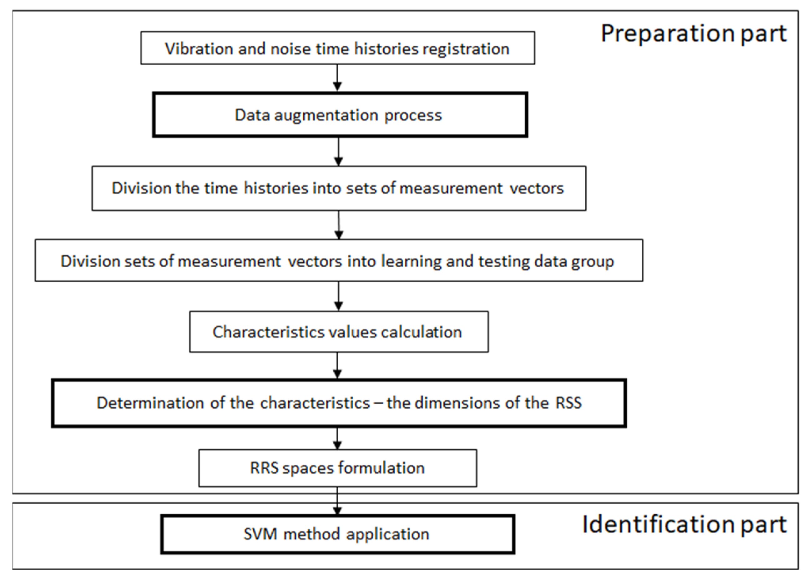
2.1. Reliability State Identification Procedure

The procedure presented in the paper is an extension of the procedure formulated as a result of the authors’ previous research, which is described in detail in Ref. [31]. It should be stressed that the procedure is a system approach to the issue under consideration and can be implemented to identify the reliability state of any rotating system.

The structure of the previously prepared method is presented in Figure 1.

In order to increase the method efficiency and robustness, the preparation phase was extended by a data augmentation process. Additionally, selection of the characteristics—the dimensions of the reliability (RSS) and inability (ISS) states spaces—was accomplished by correlation analysis between all characteristics using the Pearson correlation coefficient. The identification phase of the procedure was also modified. In the new variant, identification was performed using the SVM method. The structure of the new identification procedure is presented in Figure 2.

The core element of the proposed procedure is the reliability states space formulation. In the space, each time history result of the vibration and noise signal recorded for the research object while it is in a specified reliability state is expressed as a point. The dimensions of such a space are the signals’ time histories and the reliability state of the system. Thus, the formulated space is the functional space in which individual dimensions are the time functions.

Identification of the reliability state and the type of the inability state, regardless of the method used, generally involves the calculation of the distance between points in the formulated space. The distance calculation in the functional space can be complicated and time consuming. Therefore, it was proposed to substitute each time history with its characteristics calculated according to the following formulas [33]:

$$\left[{vs}_i\right]=\underset{t_0}{\overset{t_k}{\int }}{vs}_i\left(t\right)dt$$

(1)

$$〈{vs}_i〉=\frac{1}{t_k-t_0}\underset{t_0}{\overset{t_k}{\int }}{vs}_i\left(t\right)dt$$

(2)

$$E_{vsi}=\underset{t_0}{\overset{t_k}{\int }}{{vs}_i}^2\left(t\right)dt$$

(3)

$$P_{vsi}=\frac{1}{t_k-t_0}\underset{t_0}{\overset{t_k}{\int }}{{vs}_i}^2\left(t\right)dt$$

(4)

$$\overline{{m^1}_{vsi}}=\underset{t_0}{\overset{t_k}{\int }}t·{vs}_i\left(t\right)dtp\left({RS}_i\right)$$

(5)

$$\overline{{m^2}_{vsi}}=\underset{t_0}{\overset{t_k}{\int }}{t}^2·{vs}_i\left(t\right)dt$$

(6)

$${\left(\overline{t-\overline{m_{vsi}}}\right)}^1=\underset{t_0}{\overset{t_k}{\int }}\left(t-\overline{m_{vsi}}\right)·{vs}_i\left(t\right)dt$$

(7)

$${\left(\overline{t-\overline{m_{vsi}}}\right)}^2=\underset{t_0}{\overset{t_k}{\int }}{\left(t-\overline{m_{vsi}}\right)}^2·{vs}_i\left(t\right)dt$$

(8)

$$\overline{t_{vsi}^1}=\frac{{\int }_{t_0}^{t_k}t·{vs}_i\left(t\right)dt}{{\int }_{t_0}^{t_k}{vs}_i\left(t\right)dt}$$

(9)

$$\overline{t_{vsi}^2}=\frac{{\int }_{t_0}^{t_k}{t}^2·{vs}_i\left(t\right)dt}{{\int }_{t_0}^{t_k}{vs}_i\left(t\right)dt}$$

(10)

$${\left(\overline{t-\overline{t_{vsi}}}\right)}^1=\frac{{\int }_{t_0}^{t_k}\left(t-\overline{t_{vsi}}\right)·{vs}_i\left(t\right)dt}{{\int }_{t_0}^{t_k}{vs}_i\left(t\right)dt}$$

(11)

$${\left(\overline{t-\overline{t_{vsi}}}\right)}^2=\frac{{\int }_{t_0}^{t_k}{\left(t-\overline{t_{vsi}}\right)}^2·{vs}_i\left(t\right)dt}{{\int }_{t_0}^{t_k}{vs}_i\left(t\right)dt}$$

(12)

$$\overline{t_{{vsi}^2}^{}}=\frac{{\int }_{t_0}^{t_k}t·{{vs}_i}^2\left(t\right)dt}{{\int }_{t_0}^{t_k}{{vs}_i}^2\left(t\right)dt}$$

(13)

$${\sigma }_{{vsi}^2}^2=\frac{{\int }_{t_0}^{t_k}{\left(t-\overline{t_{{vsi}^2}}\right)}^2{{vs}_i}^2\left(t\right)dt}{{\int }_{t_0}^{t_k}{{vs}_i}^2\left(t\right)dt}$$

(14)

$${\mathsf{\Delta }t}_{vsi}=\frac{{\int }_{t_0}^{t_k}{vs}_i\left(t\right)dt}{{vs}_i\left(0\right)}$$

(15)

$${\mathsf{\Delta }T}_{vsi}=\sqrt{\frac{{\int }_{t_0}^{t_k}{\left(t-\overline{t_{{vsi}^2}}\right)}^2·{{vs}_i}^2\left(t\right)dt}{{\int }_{t_0}^{t_k}{{vs}_i}^2\left(t\right)dt}}$$

(16)

where vs_i is the i-th recorded vibration or noise signal, t₀ is the time of the beginning of the signal vs, t_k is the time of the end of the signal vs, 1 is the integral of the signal, 2 is the mean value of the signal, 3 is the energy of the signal, 4 is the medium power of the signal, 5 is the first order simple moment, 6 is the second order simple moment, 7 is the first order central moment, 8 is the second order central moment, 9 is the normalized first order simple moment, 10 is the normalized second order simple moment, 11 is the normalized first order central moment, 12 is the second order normalized central moment, 13 is the abscissa of the signal square gravity center, 14 is the variance of the signal square, 15 is the equivalent diameter of the signal, and 16 is the mean width of the signal.

The characteristics are the basic parameters used in signal analysis. In order to determine the usefulness of the specified characteristic in the identification process, its concentration can be calculated. The characteristic is treated as concentrated if the standard deviation (σ) of the characteristic value (D) in a group of time series recorded for the same reliability state (DSG) is lower than 15% of the mean value (17).

$${\sigma }_{D\left(DSG\right)}\le \overline{\mathrm{D}}\left(\mathrm{D}\mathrm{S}\mathrm{G}\right)·0.15$$

(17)

where D(DSG) is the characteristic of the signal, and DSG is the group of the time series recorded for the same reliability state.

Additionally, it is assumed that:

• The characteristic can be used to uniquely identify the reliability state if it fulfills the condition described by Formula (18);
• The characteristic can be used to uniquely identify the type of the inability state if it fulfills the condition described by Formula (19) for all inability states.

$${\sigma }_{D\left({DSG}_{IA}\right)}+{\sigma }_{D\left({DSG}_A\right)}\le \left|\overline{\mathrm{D}}\left({\mathrm{D}\mathrm{S}\mathrm{G}}_{IA}\right)-\overline{\mathrm{D}}\left({\mathrm{D}\mathrm{S}\mathrm{G}}_A\right)\right|$$

(18)

where D(DSG) is the characteristic of the signal, DSG_IA is the group of time series recorded for the inability states, and DSG_A is the group of time series recorded for the ability states.

$${\sigma }_{D\left({DSG}_{IA}^i\right)}+{\sigma }_{D\left({DSG}_{IA}^j\right)}\le \left|\overline{\mathrm{D}}\left({DSG}_{IA}^i\right)-\overline{\mathrm{D}}\left({DSG}_{IA}^j\right)\right|$$

(19)

where D(DSG) is the characteristic of the signal, and DSG_IAⁱ is the group of time series recorded for the i-th inability state.

Due to the performed substitution, the functional RSS n+1 dimensional space (n is number of signals) was transformed into a Cartesian 16n+1 dimensional space in which distance can be calculated as Euclidean. However, the number of the dimensions significantly increased (16 times per signal time history dimension). Therefore, the next phase of the procedure was the characteristics determination—the dimensions of the RSS step. It should be noted that some of the characteristics are linearly dependent and can be easily excluded from further consideration, but in order to check the effectiveness of the characteristics determination step, it was decided not to exclude them.

In the formulated reliability states space, the identification of the reliability state and the type of the inability state of the considered technical system took place according to the selected classification method.

2.2. Data Preprocessing

Data preprocessing performed during the presented research comprised data augmentation and reducing the number of characteristics used to formulate the RSS space.

Data augmentation is a common practice in image recognition, but it is not standard procedure in the case of time series analysis [34]. Generally, data augmentation techniques can be divided into four groups: random transformations, pattern mixing, generative models, and decomposition [35]. For time series, random transformations are usually used. In the literature, methods such as adding random noise [36], slicing [37], scaling [38], rotation [39], or warping in the time and frequency domain [40] can all be found.

The research conducted involves vibration and noise signal analysis in the time domain; therefore, only slicing, permutation, and time warping were taken into consideration. In order to select proper augmentation techniques, the general concept of the proposed method of fault identification should be taken into account. As previously mentioned, it is the classification issue based on the distance calculation in the space formulated by the characteristics calculated for each of the diagnostic signals [31]. The usefulness of a given characteristic in the classification process depends on its concentration. Therefore, the data augmentation should not decrease the characteristics’ concentration; however, the time dependencies of the measurement vectors (values of signals recorded for the same time t) do not require strict preservation. Thus, slicing and permutation in the form of random shuffling [41] were employed.

Random shuffling involves randomly rearranging the measurement vectors in a time series. As a result, new time histories are obtained. This multiplies the amount of data by two.

Slicing by time window with overlapping consists of slicing the time signal using a time window of defined length and moving the window along the signal. If the window movement is shorter than the window length, the number of samples received is greater than the number of samples that can be obtained by splitting the signal into pieces.

The reduction in the number of characteristics was accomplished by correlation analysis between every characteristic using the Pearson correlation coefficient [42] (20).

$$r_{ij}=\frac{{\sum }_{k=1}^{card\left({DS}_{learning}\right)}\left(D_i^k-{\overline{D}}_i\right)·\left(D_j^k-{\overline{D}}_j\right)}{\sqrt{{\sum }_{k=1}^{card\left({DS}_{learning}\right)}{\left(D_i^k-{\overline{D}}_i\right)}^2}·\sqrt{{\sum }_{k=1}^{card\left({DS}_{total}\right)}{\left(D_j^k-{\overline{D}}_j\right)}^2}}$$

(20)

where r_ij is the sample Pearson correlation coefficient between the i-th and j-th characteristic, DS_learning is the set of the data samples, and D^K_i is the value of the i-th characteristics for the k-th data sample.

2.3. Identification Model—Support Vector Machine Method

During the present research, vibration and noise signals were recorded for the object while it was in a known reliability state, so the most accurate method to build the identification model was the supervised learning approach. In the literature, several machine learning models and algorithms used in classification issues can be found. The most common are stochastic gradient descent (SGD) [43], SVM [44], decision tree (DT) [45], and random forest (RF) [46]. SVM has been widely used within the maritime domain for the fault diagnosis of marine machinery. In Ref. [47], the SVM method was applied to identify deviant, abnormal ship machinery conditions, while in Ref. [48], it was used to perform fault diagnoses of the fuel, lubrication, intake and exhaust, and cooling subsystems of the ship’s diesel engine structure. One of the reasons for SVM application in vibration analysis for machine diagnosis is its compatibility with large and complex data sets [49]. Importantly, SVM performance (in terms of complexity and computation time) is not affected by the number of features of the classified entities [50]; therefore, there is no limitation to the number of selected attributes used in the classification process. Additionally, as SVM is one of the system methods, there is no requirement for expert knowledge specific to the analyzed domain in order to build the SVM model. However, it should be kept in mind that in cases where the number of features for each data point exceeds the number of training data samples, the quality of the SVM model response will be lower. Taking into consideration the industrial applicability and simplicity of the machine learning model, the SVM method was selected for use in the current study.

The support vector machine (SVM) is a powerful and versatile machine learning model, able to carry out linear or non-linear classification. It is one of the most popular machine learning solutions, commonly used in engineering applications [51,52,53]. It is especially useful for classifying complex, small, or medium-sized data sets. One of the research objectives is to propose the procedure for reliability states identification in the case of a limited data set. Therefore, it was decided to use SVM modeling to solve the problem under consideration.

The fundamental concept of SVM modeling is to determine the optimal hyperplane in order to separate data samples of different classes. The SVM classifier determines the class of the data sample by computing the decision function value (21):

$$F_d=W^T·X+b=w_1·x_1+w_2·x_2+\cdots +w_n·x_n+b$$

(21)

where F_d is the decision function, w_i is the weight of the feature, x_i is the value of the feature, and b is the bias.

The main objective of the SVM model learning process is to determine the values of the weights, which provides the maximum distance between the hyperplane and the samples.

In the case of the issue in which linear classification cannot be used, an SVM variant with polynomial kernel (22) implementation can be applied. The kernel is used to transform the calculation of the bias and decision function values:

$$K(X_1,X_2)={(a+X_1^T·X_2)}^b$$

(22)

where K is the kernel, a is the constant term, and b is the degree of the kernel.

The SVM classifier is binary; therefore, to identify several classes of data samples, the One-versus-One (OvO) strategy was applied. It consists of learning N(N−1)/2 classifiers to compare classes to each other, where N is the number of classes. The obtained class of the analyzed sample is the one that wins in most comparison cases. The main advantage of the OvO strategy is the fact that each classifier needs to be trained only for the portion of the learning set consisting of both compared classes. The SVM algorithm does not scale well to the size of the learning data set. Therefore, it is preferable to use the OvO strategy in the SVM case because in this strategy, many classifiers are trained for small data sets, and it is faster than training several classifiers against large collections of samples [54].

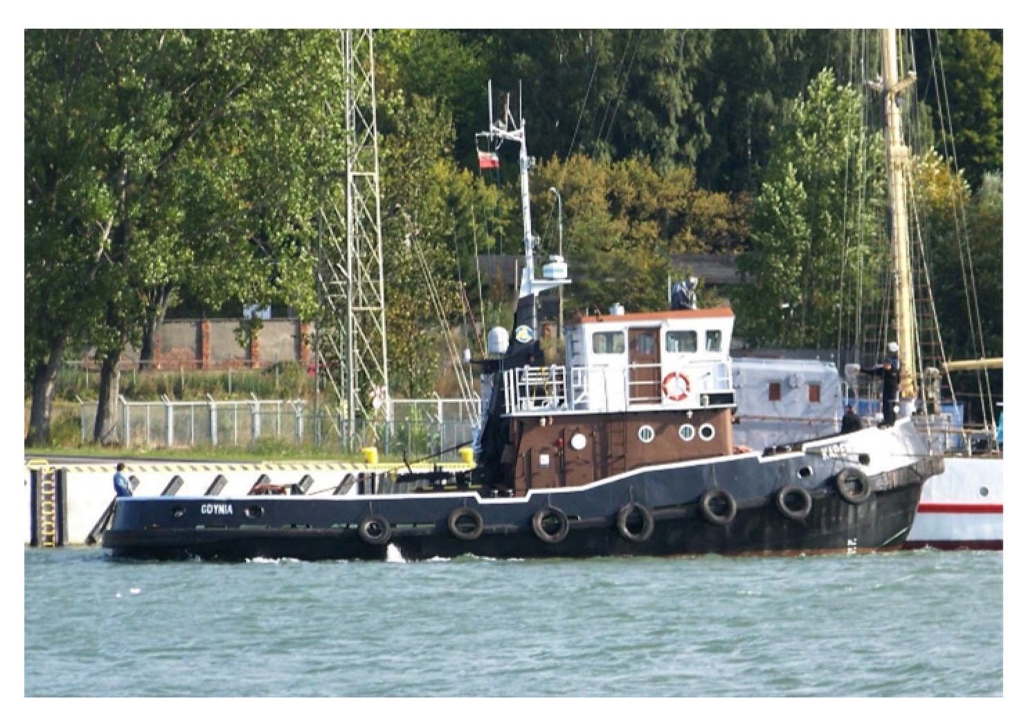
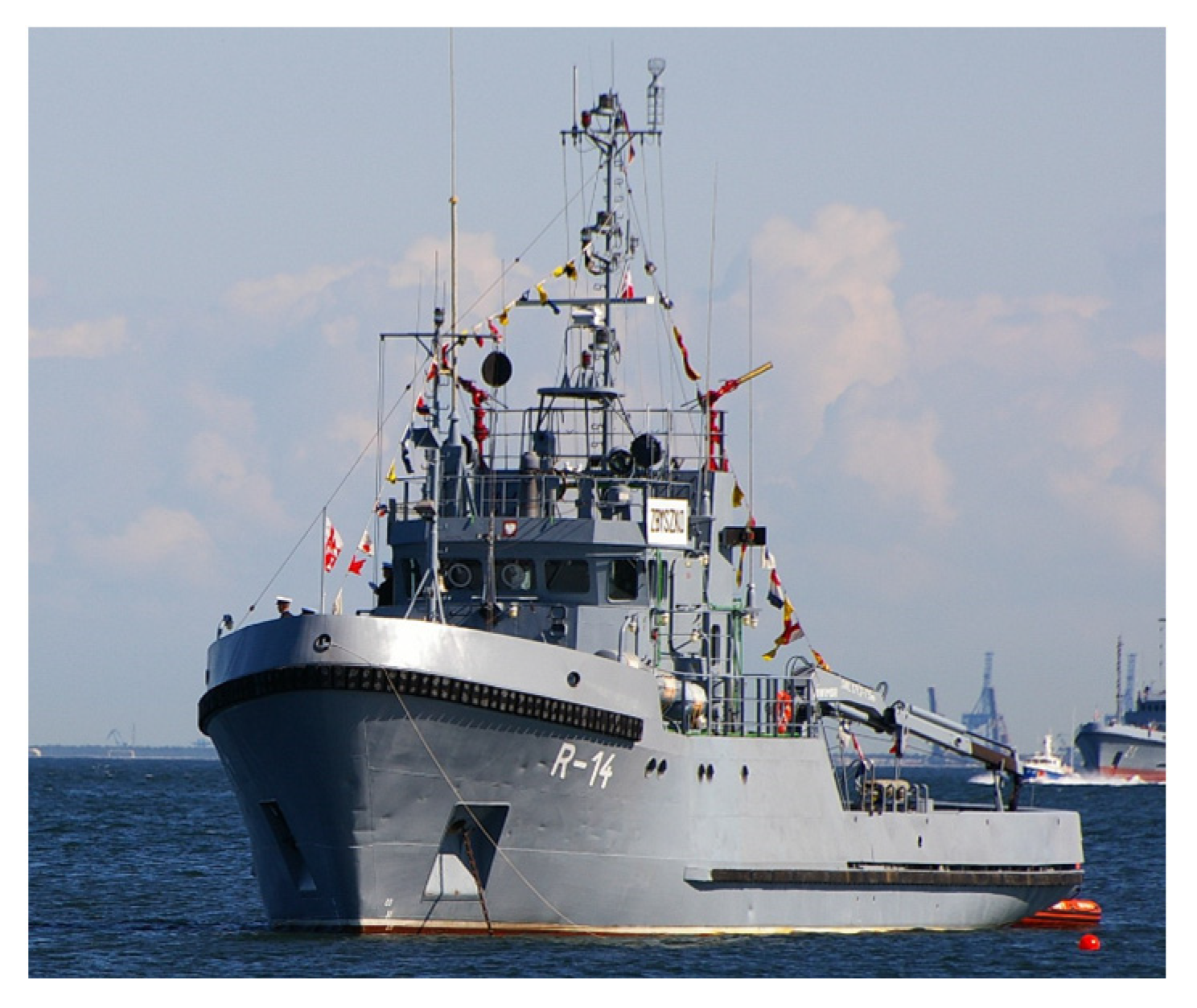
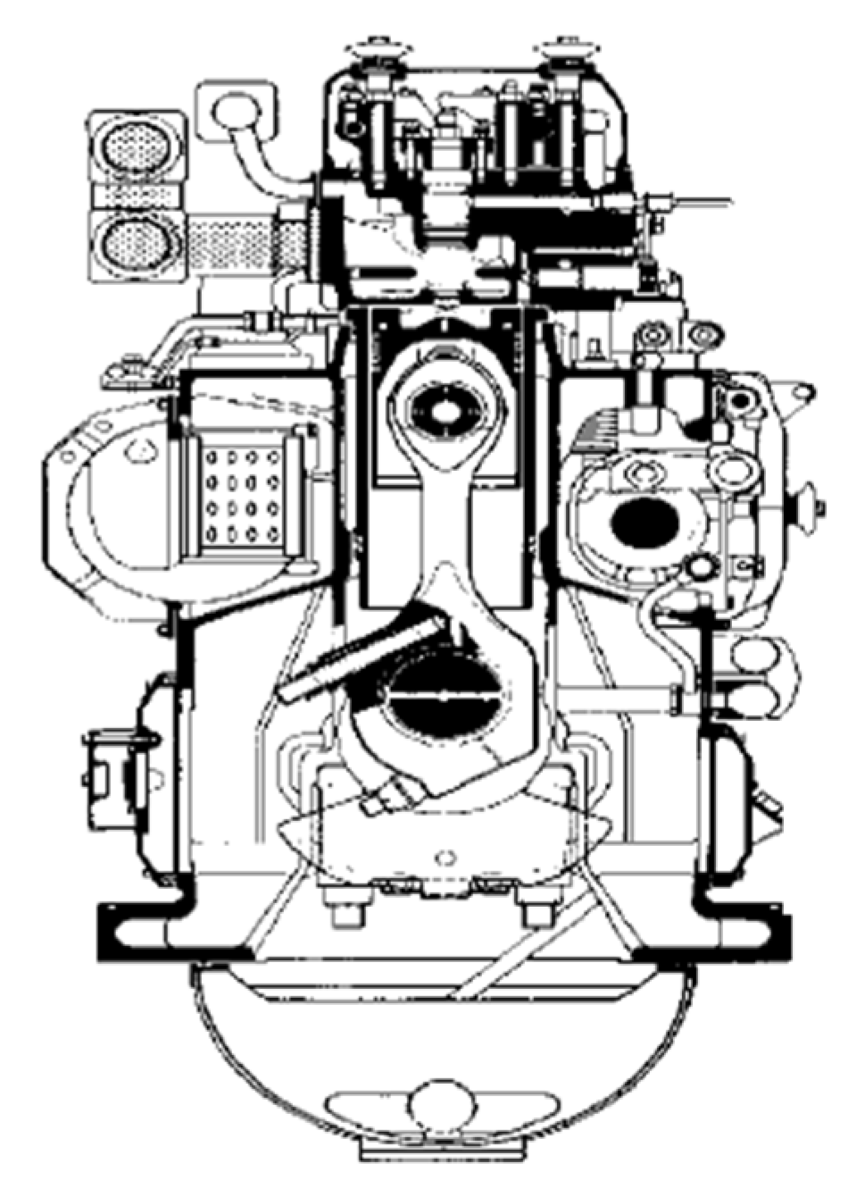
3. Research Object and Performed Operational Tests

The research object was the Sulzer 6AL20/24 marine engine produced by Zakłady Przemysłu Metalowego (ZPM) H.Cegielski in Poznań, Poland. Most of these engines work as auxiliary power generators on ships, while some are used as a stationary power source (especially popular in India, as recovered from scrapped ships and rebuilt), and many are employed as the main propulsion in tugs, floating cranes, fishing ships, and other workboats. In Poland, this type of engine is often used in civil (Figure 3) and navy (Figure 4) vessels.

The engine under testing was equipped with a Woodward PGA-type multi-scope rotational speed controller. Thus, the rotational speed could vary in the range of 700–1200 rpm. The AL20 series engines can be fired by heavy fuel oil (HFO), marine diesel oil (DMO), or gas. The diameter of the cylinder was 200 mm, the stroke was 300 mm, and the nominal value of the valve clearances was 0.4 mm (Figure 5). The basic engine specifications are presented in

Table 1. Basic technical specifications of Sulzer 6 AL 20/24 engine.

Parameter	Value	Unit
Cylinder diameter	200	mm
Cylinder stroke	240	mm
Displacement volume of one cylinder	7450	cm3
Compression ratio	1:12.7	-
Nominal rotational speed	750	rpm
Mean piston velocity	6	m/s
Nominal load	420	kW
Mean effective pressure	1.693	MPa
Pressure of injection	24.5	MPa
Maximum combustion pressure	12.95	MPa

.

The operational tests were performed on a laboratory stand, which was placed in a ship engine room laboratory of the Mechanical and Electrical Engineering Department of the Polish Naval Academy in Gdynia (Figure 6).

The tests consisted of recording vibration and noise signals generated by the engine working in both the ability state and different inability states. The tests were conducted under the same values of the operating parameters. The rotational speed was about 750 rpm, and the torque was 3.3 kNm. The vibration signals (vertical and horizontal directions) were measured using a head placed on each cylinder. The measurements of noise intensity were carried out by a microphone positioned 200 cm from the engine. The sampling frequency was 32,768 Hz. During the tests, five different failures were simulated, according to the following list:

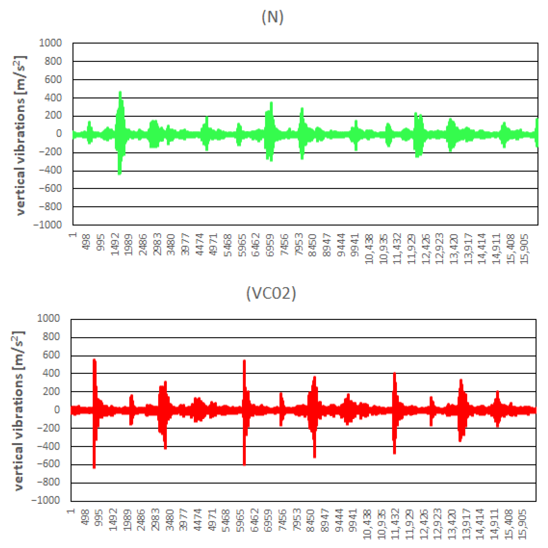
• VC02—operation of the engine with input and output valve clearances reduced to 0.2 mm for cylinder 4, and output valve clearances increased up to 1 mm for cylinder 1;
• VC08—operation of the engine with input and output valve clearances increased up to 0.8 mm for cylinder 4, and output valve clearances increased up to 1 mm for cylinder 1;
• CLE—operation of the engine with output valve clearances increased up to 1 mm for cylinder 1;
• PUMP—operation of the engine with simulated damage to the injection pump of cylinder 1—the maximal combustion pressure dropped by about 20, and the output valve clearances increased up to 1 mm for cylinder 1;
• INJ—operation of the engine with the opening pressure injector of cylinder 1 decreased to 23 MPa, and the output valve clearances increased up to 1 mm for cylinder 1.

For each reliability state for each cylinder, the vertical and horizontal vibrations and noise intensity were recorded. Thus, the total number of diagnostic signals can be calculated as the number of cylinders equal to six, multiplied by the number of diagnostic signals recorded for each cylinder (three, i.e., vertical vibrations, horizontal vibrations, and noise intensity), resulting in 18 signals for each reliability state.

4. Recorded Data Preprocessing

The values of all 18 measured signals recorded for a specified time t comprise a measurement vector. Each recorded time history of the measured signals (18 combined signals) was divided into 0.5 s sequences of measurement vectors (sets of 16384 consecutive measurement vectors).

In Figure 7, one of the 18 signals (vertical vibrations for cylinder 1) of the exemplary set of measurement vectors is presented for the ability (N) and selected inability (VC02) states. In this way, 28 sets for states N, VC02, and VC08; 29 sets for state CLE; 26 sets for state INJ; and 13 sets for the PUMP state were obtained. From a machine learning perspective, each set of measurement vectors is a labeled sample.

Based on previous studies [56,57,58] and our own experience, it was determined that the number of samples was not sufficient to prepare a machine learning model. This situation is very common in real industrial systems in which the amount of data is limited. Therefore, it was decided not to increase the length of the recorded time histories, but to solve the problem by augmenting the data.

In the beginning, for each recorded time history, random shuffling was applied. This multiplied the data amount by two. Subsequently, slicing by time window, with overlapping, was executed. The length of the window was 16,384 measurement vectors (assumed length of a sample), and the shift of the window was 10% of the window length (1638 measurement vectors). Each time history was extended by 16,384 measurement vectors, copied from the beginning, in order to include all the data into the resulting measurement vector sets. Thanks to the performed data augmentation, the number of measurement vector sets increased 20 times, which yielded 562 sets for states N, VC02, and VC08; 582 sets for state CLE; 522 sets for state INJ; and 262 sets for the PUMP state.

After data augmentation, the characteristics for each signal were calculated. Next, each set of measurement vectors was substituted with the values of the calculated characteristics. In this way, labeled data samples were obtained in the form of 288 features (16 characteristics multiplied by 6 cylinders multiplied by 3 signals: horizontal vibrations, vertical vibrations, and intensity of noise) and the label describing the reliability state and the type of failure for which the sample was recorded (23).

$${DS}_i={[V1:1÷16,H1:1÷16,N1:1÷16,\cdots ,V6:1÷16,H6:1÷16,N6:1÷16,RS]}^T$$

(23)

where DS_i is the i-th data sample, Vj:k is the value of k-th characteristics calculated for the j-th cylinder for a vertical vibration signal, Hj:k is the value of the k-th characteristics calculated for the j-th cylinder for a horizontal vibration signal, Nj:k is the value of the k-th characteristics calculated for the j-th cylinder for a noise signal, and RS is the reliability state.

The data samples were divided into two sets, the learning and the testing set, with an 80/20 ratio. The samples for the testing set were selected at random; however, the proportions of individual categories (reliability states) were maintained as they existed in the total set. To check whether the selection maintained the correct category distribution, the share of each reliability state in the total and test sets, along with their errors, have been calculated according to Formulas (24) and (25) (

Table 2. Accuracy of testing set selection.

Reliability State	p(RSi)test	p(RSi)total	serr[%]
N	0.183306	0.184142	0.453722
VC02	0.184943	0.184142	0.435084
VC08	0.184943	0.184142	0.435084
CLE	0.191489	0.190695	0.416758
INJ	0.170213	0.171035	0.480965
PUMP	0.085106	0.085845	0.416758

).

$$p\left({RS}_i\right)=\frac{card\left({DSG(RS}_i\right))}{\sum _{i}card\left({DSG(RS}_i\right))}$$

(24)

where p(RS_i) is the share of the i-th reliability state, DSG(RS_i) is the group of samples of the i-th reliability state, and card is the cardinality of a set.

$$s_{err}\left({RS}_i\right)=\frac{\left|{p\left({RS}_i\right)}_{test}-{p\left({RS}_i\right)}_{total}\right|}{{p\left({RS}_i\right)}_{total}}·100\%$$

(25)

where s_err(RS_i) is the error of selection, RS_i is the i-th reliability state, p(RS_i)_test is the share of the i-th reliability state in the test set, and p(RS_i)_total is the share of the i-th reliability state in the total set.

In order to check the influence of data augmentation on the concentration of the characteristics, the concentration of each characteristic for each reliability state was calculated (17) separately for the original, transformed, and original + transformed samples using the learning data set.

Despite a slightly lower concentration of characteristics for the transformed samples for some signals (especially noise signals) in reference to the original samples, for original and transformed samples together, the concentration was even higher. Therefore, it was proposed that augmentation could be applied for the considered classification issue. The detailed results of the comparison are presented in

Table 3. The number of concentrated characteristics for the original and transformed samples.

Reliability State	Original Samples *	Transformed Samples *	Original and Transformed Samples *
N	V:30|H:27|N:9	V:30|H:29|N:8	V:30|H:29|N:8
VC02	V:28|H:21|N:10	V:29|H:30|N:10	V:29|H:30|N:10
VC08	V:30|H:24|N:71	V:30|H:30|N:68	V:30|H:30|N:70
CLE	V:24|H:21|N:11	V:30|H:29|N:10	V:30|H:29|N:11
INJ	V:28|H:24|N:9	V:29|H:29|N:9	V:30|H:29|N:10
PUMP	V:29|H:24|N:11	V:29|H:30|N:10	V:29|H:29|N:11

* Presentation—type of signal: number of concentrated characteristics.

.

Additionally, each concentrated characteristic was analyzed from the point of view of the identification of the reliability states (18) and the types of inability states (19).

In the case of the reliability state identification, there were two concentrated characteristics which fulfilled the condition (18): the energy and the medium power of the horizontal vibrations recorded on cylinder 4. In the case of the identification of the type of inability state, there were no concentrated characteristics that fulfilled the condition (19) calculated between every type of inability state. This means that the considered classification issue is not a linear one; thus, no linear classifier can be used in the conducted research.

The next step in the data analysis was the reduction in the characteristic number. This was accomplished by conducting a correlation analysis between each characteristic using the Pearson correlation coefficient (20). In Figure 8, the diagrams of the exemplary correlated and non-correlated characteristics can be found.

It can be easily seen that in the case of correlated characteristics (V1:5 = f(V1:1)—the simple moment of the first order of vertical vibrations of cylinder 1 expressed as a function of the integral of vertical vibrations of cylinder 1), they show some degree of linear dependence. In contrast, in the case of non-correlated characteristics (V1:16 = f(V1:13)—the mean width of vertical vibrations of cylinder 1 expressed as a function of the abscissa of the vertical vibrations of the cylinder 1 square gravity center), the distribution of the points is undirected. If the value of the correlation coefficient between two characteristics was equal to or higher than 0.8, one of them was excluded from further consideration. In this way, the number of the characteristics was decreased to 157 according to the following list:

• For vertical vibrations, characteristics number 1,3,7,8,9,11,12,13,14,15 for each cylinder;
• For horizontal vibrations, characteristics number 1,3,7,8,9,11,12,13,14,15 for each cylinder;
• For noise signal, characteristics number 9,11,12,13,14,15 for each cylinder and characteristic number 1 for cylinder 1.

It should be noted that all linearly dependent characteristics were detected and excluded from further analysis.

Because most machine learning algorithms perform poorly with numerical attributes within different ranges of the scale, the last step of the data preparation was a sample standardization. This was accomplished by mean value subtraction and division by standard deviation according to Formula (26)

$${D\prime }_i^k=\frac{D_i^k-{\overline{D}}_i}{{\sigma }_{D_i}}$$

(26)

where D’^K_i is the value of the i-th characteristic for the k-th data sample after standardization, D_i is the i-th characteristic of the signal, and D^K_i is the value of the i-th characteristic for the k-th data sample.

Subsequently, the data samples prepared by the method presented above were used to identify the reliability state and the type of inability state using the machine learning model.

5. Results

During the data analysis (described in the previous chapter), it was stated that the identification of the reliability state and the type of inability state are issues for which linear classification cannot be used. Therefore, a non-linear variant of SVM was applied (SVM variant with polynomial kernel). As has been previously mentioned, the SVM classifier is binary; therefore, to identify several classes of data samples (one ability state and five types of inability state), the One-versus-One (OvO) strategy was used.

In order to preliminarily check the performance of the non-linear SVM classifier with polynomial kernel (P-SVM), the k-fold cross-validation procedure was used. According to the procedure, the learning set is randomly divided into k folds, and the model is trained and evaluated k times (a different subset is selected each time to evaluate the performance of the model, and the remaining k-1 are used for training). Finally, the k evaluation results are obtained. In this research, k was equal to 3 (scikit-learn Python library default value), and the performance was assessed in regards to accuracy (correct classifications for all classification ratios). For default values of the model, the mean accuracy of the hyper-parameters was 83%.

The P-SVM model includes several hyper-parameters, the most significant being the degree of kernel, the constant term of the kernel, and the regularization parameter, which is used to avoid model overfitting. The strength of the regularization is inversely proportional to the C parameter. In order to determine the best values of the hyper-parameters, the grid search method was used. Using this method, for all combinations of the entered values of the hyper-parameters, the model performance was evaluated by the k-fold cross-validation procedure. The following values of the hyper-parameters were used:

• The degree of kernel: 3,6,9;
• The constant term of the kernel: 1, 10, 100;
• The regularization parameter: 1, 3, 5.

The values of the hyper-parameters were selected arbitrarily in order to determine the search subspace in which further tuning will take place. Specifying the number of folds equal to 3, the best combination was obtained in the following form: 3, 1, and 1, respectively. For the resulting values of the hyper-parameters, the mean accuracy of the model obtained by the k-fold cross-validation procedure was equal to 0.999. Because a very high value of obtained accuracy was achieved, it was determined that an additional tuning process was not necessary. The model is well trained, and its performance can be checked using the testing data set.

The confusion matrix of the model operation over the testing data set (

Table 4. The confusion matrix of the model operation.

Actual Values	Predicted Values
Reliability State	N	VC02	VC08	CLE	INJ	PUMP
N	112	0	0	0	0	0
VC02	0	112	0	0	0	0
VC08	0	0	112	0	0	0
CLE	0	0	0	116	0	0
INJ	0	0	0	0	104	0
PUMP	0	0	0	0	0	52

) only exhibited non-zero values on the main diagonal; therefore, the evaluation metrics [59], including accuracy, precision, recall, selectivity, and F1 score, were equal to 100%.

In each case, the optimum degree of the kernel was 3, the optimum constant term of the kernel was 1, and the optimum regularization parameter was 1. Then, each learning set was used to train the P-SVM model. The performance of the resulting models was tested using the full testing data set, in which the labels were changed to distinguish only the ability and inability state. As a result, 100% accuracy was obtained in each case.

6. Discussion and Conclusions

During the presented studies, a new universal procedure for reliability state identification was proposed. The procedure is a systematic approach to the identification of the ability and the type of inability state of a complex technical system.

The proposed method was applied to identify the ability state and the type of the inability state of a Sulzer 6AL20/24 marine engine. Using data science techniques to analyze vibration and noise signals recorded during the operational tests, along with machine learning modeling in the form of a non-linear SVM classifier with a polynomial kernel, 100% accuracy was obtained in regards to the identification process. Moreover, the method was used to distinguish between ability and inability states in the event that testing data set signals recorded for unknown inability states were present. In this case, a 100% identification accuracy was also achieved.

Although the proposed method was applied to a specific object, it is a general approach which can be used in the identification of the ability and inability states of a wide range of technical systems—particularly in the case of rotating, complex technical systems. The elements of the method were used by the authors to identify the technical state of a rotating system on a laboratory stand [60] and the propulsion system of mine-detecting ships [61]. Currently, research is being conducted to apply the method in the case of low-speed water turbines.

As a result of the research, 100% accurate reliability state identification was obtained. Thus, it was proved that the implementation of data science techniques and machine learning modeling in the area of complex technical system diagnostics yields high quality solutions. On the other hand, obtaining an accuracy of 100% in the test set for such complex data sets, using a limited amount of data, seems to be surprising. However, analyzing the literature [62,63,64,65], it can be seen that SVM application in the area of vibration classification usually produces very good results (93.75–100% accuracy).

In contrast, the analysis of time waveform and FFT type vibration parameters (the comparative analysis of selected harmonics and their ratio values) provides information about the technical condition of the engine injection system. However, it does not provide the unambiguous indication of which injectors or injection pumps are malfunctioning [30]. The accuracy of the identification of the reliability state and the type of the inability state using a previous variant of the method [31] was 100% in the case of ability/inability state identification, 95.6% in the case of the type of inability state identification, and about 78% in the case of ability/inability state identification, with an unknown type of failure. Using a stochastic gradient descent (SGD) classifier as a classification tool in the presented method brought the accuracy to the level of 96% in the case of type of inability state identification. In the same case, thanks to the linear SVM variant application, 97% accuracy was obtained.

The quality of the obtained solution encourages further research in this area. The authors plan to verify the performance of the proposed approach in the case of the vibration and noise signals recorded during engine operation in the workplace. The second direction for further studies is to apply the method in the case in which the learning data set consists of the signals recorded on the laboratory stand, and the testing data set consists of the signals recorded in the engine workplace. If high accuracy can be achieved using such a configuration, the method will be ready for real-world application. Finally, the merging of supervised and unsupervised learning method implementation will be performed. There is a plan to train a selected machine learning model using fully labeled samples (known ability and inability states), and to use this model to identify known and unknown inability states according to new samples clusters detection.

References

1. Bayraktar, M.; Nuran, M. Reliability, availability, and maintainability analysis of the propulsion system of a fleet. Sci. J. Marit. Univ. Szczecin 2022, 70, 63–70. [Google Scholar]
2. Liu, L.; Wu, Y.; Wang, Y.; Wu, J.; Fu, S. Exploration of environmentally friendly marine power technology -ammonia/diesel stratified injection. J. Clean. Prod. 2022, 380, 135014. [Google Scholar] [CrossRef]
3. Mohd Ghazali, M.H.; Rahiman, W. Vibration Analysis for Machine Monitoring and Diagnosis: A Systematic Review. Shock Vib. 2021, 2021, 9469318. [Google Scholar] [CrossRef]
4. Ren, G.; Jia, J.; Mei, J.; Jia, X.; Han, J.; Wang, Y. An improved variational mode decomposition method and its application in diesel engine fault diagnosis. J. Vibroeng. 2018, 20, 2363–2378. [Google Scholar] [CrossRef]
5. Bianchi, D.; Mayrhofer, E.; Gröschl, M.; Betz, G.; Vernes, A. Wavelet packet transform for detection of single events in acoustic emission signals. Mech. Syst. Signal Process. 2015, 64–65, 441–451. [Google Scholar] [CrossRef]
6. Adly, A.R.; Abdel Aleem, S.H.E.; Elsadd, M.A.; Ali, Z.M. Wavelet packet transform applied to a series-compensated line: A novel scheme for fault identification. Meas. J. Int. Meas. Confed. 2020, 151, 107156. [Google Scholar] [CrossRef]
7. Yang, S.; Gu, X.; Liu, Y.; Hao, R.; Li, S. A general multi-objective optimized wavelet filter and its applications in fault diagnosis of wheelset bearings. Mech. Syst. Signal Process. 2020, 145, 106914. [Google Scholar] [CrossRef]
8. Shi, Y.; Yi, C.; Lin, J.; Zhuang, Z.; Lai, S. Ensemble empirical mode decomposition-entropy and feature selection for pantograph fault diagnosis. J. Vib. Control 2020, 26, 2230–2242. [Google Scholar] [CrossRef]
9. Cheng, Y.; Wang, Z.; Chen, B.; Zhang, W.; Huang, G. An improved complementary ensemble empirical mode decomposition with adaptive noise and its application to rolling element bearing fault diagnosis. ISA Trans. 2019, 91, 218–234. [Google Scholar] [CrossRef]
10. Jiang, X.; Wang, J.; Shi, J.; Shen, C.; Huang, W.; Zhu, Z. A coarse-to-fine decomposing strategy of VMD for extraction of weak repetitive transients in fault diagnosis of rotating machines. Mech. Syst. Signal Process. 2019, 116, 668–692. [Google Scholar] [CrossRef]
11. Li, J.; Yao, X.; Wang, H.; Zhang, J. Periodic impulses extraction based on improved adaptive VMD and sparse code shrinkage denoising and its application in rotating machinery fault diagnosis. Mech. Syst. Signal Process. 2019, 126, 568–589. [Google Scholar] [CrossRef]
12. Saidi, L.; Ben Ali, J.; Bechhoefer, E.; Benbouzid, M. Wind turbine high-speed shaft bearings health prognosis through a spectral Kurtosis-derived indices and SVR. Appl. Acoust. 2017, 120, 1–8. [Google Scholar] [CrossRef]
13. Wang, Y.; Xiang, J.; Markert, R.; Liang, M. Spectral kurtosis for fault detection, diagnosis and prognostics of rotating machines: A review with applications. Mech. Syst. Signal Process. 2016, 66–67, 679–698. [Google Scholar] [CrossRef]
14. Dhal, A.; Panigrahi, I.; Mishra, C.; Samantaray, A.K. Order Tracking: Angular Domain Features Extraction Method for Condition Monitoring of Variable Speed. In Lecture Notes in Mechanical Engineering; Springer: Berlin, Germany, 2020; pp. 127–133. [Google Scholar]
15. Wu, J.; Zi, Y.; Chen, J.; Zhou, Z. Fault diagnosis in speed variation conditions via improved tacholess order tracking technique. Meas. J. Int. Meas. Confed. 2019, 137, 604–616. [Google Scholar] [CrossRef]
16. He, G.; Ding, K.; Li, W.; Jiao, X. A novel order tracking method for wind turbine planetary gearbox vibration analysis based on discrete spectrum correction technique. Renew. Energy 2016, 87, 364–375. [Google Scholar] [CrossRef]
17. Zhang, L.; Zeng, R.; Jia, J.; Lü, L.; Zhang, G. Engine fault diagnosis based on work-cycle order tracking spectrum and fuzzy C-mean clustering. Qiche Gongcheng/Automotive Eng. 2014, 36, 1024–1028. [Google Scholar]
18. Cai, B.; Wang, Z.; Zhu, H.; Liu, Y.; Hao, K.; Yang, Z.; Ren, Y.; Feng, Q.; Liu, Z. Artificial Intelligence Enhanced Two-Stage Hybrid Fault Prognosis Methodology of PMSM. IEEE Trans. Ind. Inform. 2022, 18, 7262–7273. [Google Scholar] [CrossRef]
19. Kong, X.; Cai, B.; Liu, Y.; Zhu, H.; Yang, C.; Gao, C.; Liu, Y.; Liu, Z.; Ji, R. Fault Diagnosis Methodology of Redundant Closed-Loop Feedback Control Systems: Subsea Blowout Preventer System as a Case Study. IEEE Trans. Syst. Man Cybern. Syst. 2023, 53, 1618–1629. [Google Scholar] [CrossRef]
20. Han, Y.; Chen, S.; Gong, C.; Zhao, X.; Zhang, F.; Li, Y. Accurate SM Disturbance Observer-Based Demagnetization Fault Diagnosis With Parameter Mismatch Impacts Eliminated for IPM Motors. IEEE Trans. Power Electron. 2023, 38, 5706–5710. [Google Scholar] [CrossRef]
21. Tseng, M.L.; Wu, K.J.; Ma, L.; Kuo, T.C.; Sai, F. A hierarchical framework for assessing corporate sustainability performance using a hybrid fuzzy synthetic method-DEMATEL. Technol. Forecast. Soc. Chang. 2019, 144, 524–533. [Google Scholar] [CrossRef]
22. Xuan, Q.; Fang, B.; Liu, Y.; Wang, J.; Zhang, J.; Zheng, Y.; Bao, G. Automatic Pearl Classification Machine Based on a Multistream Convolutional Neural Network. IEEE Trans. Ind. Electron. 2018, 65, 6538–6547. [Google Scholar] [CrossRef]
23. Mboo, C.P.; Hameyer, K. Fault diagnosis of bearing damage by means of the linear discriminant analysis of stator current features from the frequency selection. IEEE Trans. Ind. Appl. 2016, 52, 3861–3868. [Google Scholar] [CrossRef]
24. Hu, N.; Chen, H.; Cheng, Z.; Zhang, L.; Zhang, Y. Fault Diagnosis for Planetary Gearbox Based on EMD and Deep Convolutional Neural Networks. Jixie Gongcheng Xuebao/J. Mech. Eng. 2019, 55, 9–18. [Google Scholar] [CrossRef]
25. Li, J.; Deng, Y.; Sun, W.; Li, W.; Li, R.; Li, Q.; Liu, Z. Resource Orchestration of Cloud-Edge–Based Smart Grid Fault Detection. ACM Trans. Sen. Netw. 2022, 18, 1–26. [Google Scholar] [CrossRef]
26. Kolar, D.; Lisjak, D.; Pająk, M.; Gudlin, M. Intelligent Fault Diagnosis of Rotary Machinery by Convolutional Neural Network with Automatic Hyper-Parameters Tuning Using Bayesian Optimization. Sensors 2021, 21, 2411. [Google Scholar] [CrossRef] [PubMed]
27. Agrawal, P.; Jayaswal, P. Diagnosis and Classifications of Bearing Faults Using Artificial Neural Network and Support Vector Machine. J. Inst. Eng. Ser. C 2020, 101, 61–72. [Google Scholar] [CrossRef]
28. Wang, H.; Ren, B.; Song, L.; Cui, L. A Novel Weighted Sparse Representation Classification Strategy Based on Dictionary Learning for Rotating Machinery. IEEE Trans. Instrum. Meas. 2020, 69, 712–720. [Google Scholar] [CrossRef]
29. Min, H.; Fang, Y.; Wu, X.; Lei, X.; Chen, S.; Teixeira, R.; Zhu, B.; Zhao, X.; Xu, Z. A fault diagnosis framework for autonomous vehicles with sensor self-diagnosis. Expert Syst. Appl. 2023, 224, 120002. [Google Scholar] [CrossRef]
30. Grządziela, A.; Kluczyk, M. A Non-invasive Method of Marine Engines Fuel System Diagnostics. Pomor. Zb. 2020, 3, 381–388. [Google Scholar] [CrossRef]
31. Pająk, M.; Muślewski, Ł.; Landowski, B.; Kałaczyński, T.; Kluczyk, M.; Kolar, D. Identification of Reliability States of a Ship Engine of the Type Sulzer 6AL20/24. SAE Int. J. Engines 2021, 15, 03-0015–04-0028. [Google Scholar] [CrossRef]
32. Huang, N.; Chen, Q.; Cai, G.; Xu, D.; Zhang, L.; Zhao, W. Fault Diagnosis of Bearing in Wind Turbine Gearbox Under Actual Operating Conditions Driven by Limited Data with Noise Labels. IEEE Trans. Instrum. Meas. 2021, 70, 1–10. [Google Scholar] [CrossRef]
33. Jerzy, S. Fundamentals of the Signal Theory; WKŁ: Warszawa, Poland, 2007. [Google Scholar]
34. Wen, Q.; Sun, L.; Yang, F.; Song, X.; Gao, J.; Wang, X.; Xu, H. Time Series Data Augmentation for Deep Learning: A Survey. In Proceedings of the Thirtieth International Joint Conference on Artificial Intelligence, Montreal, QC, Canada, 7–15 January 2020. [Google Scholar] [CrossRef]
35. Iwana, B.K.; Uchida, S. An empirical survey of data augmentation for time series classification with neural networks. PLoS ONE 2021, 16, e0254841. [Google Scholar] [CrossRef]
36. Fields, T.; Hsieh, G.; Chenou, J. Mitigating Drift in Time Series Data with Noise Augmentation. In Proceedings of the 2019 International Conference on Computational Science and Computational Intelligence (CSCI), Las Vegas, NV, USA, 5–7 December 2019; pp. 227–230. [Google Scholar]
37. Le Guennec, A.; Malinowski, S.; Tavenard, R. Data augmentation for time series classification using convolutional neural networks. In Proceedings of the ECML/PKDD Workshop on Advanced Analytics and Learning on Temporal Data, Riva del Garda, Italy, 19 September 2016. [Google Scholar]
38. Um, T.T.; Pfister, F.M.J.; Pichler, D.; Endo, S.; Lang, M.; Hirche, S.; Fietzek, U.; Kulić, D. Data augmentation of wearable sensor data for parkinson’s disease monitoring using convolutional neural networks. In Proceedings of the 19th ACM International Conference on Multimodal Interaction, Glasgow, UK, 13–17 November 2017; ACM: New York, NY, USA, 2017; pp. 216–220. [Google Scholar]
39. Ruan, D.; Zhang, F.; Yan, J. Transfer Learning Between Different Working Conditions on Bearing Fault Diagnosis Based on Data Augmentation. IFAC-PapersOnLine 2021, 54, 1193–1199. [Google Scholar] [CrossRef]
40. Nguyen, T.-S.; Stuker, S.; Niehues, J.; Waibel, A. Improving Sequence-To-Sequence Speech Recognition Training with On-The-Fly Data Augmentation. In ICASSP 2020—2020 IEEE International Conference on Acoustics, Speech and Signal Processing (ICASSP), Proceedings of the ICASSP 2020 Table of Contents, Barselona, Spain, 4–8 May 2020; IEEE: Piscataway, NJ, USA, 2020; pp. 7689–7693. [Google Scholar]
41. Steven Eyobu, O.; Han, D.S. Feature Representation and Data Augmentation for Human Activity Classification Based on Wearable IMU Sensor Data Using a Deep LSTM Neural Network. Sensors 2018, 18, 2892. [Google Scholar] [CrossRef]
42. Temizhan, E.; Mirtagioglu, H.; Mendes, M. Which Correlation Coefficient Should Be Used for Investigating Relations between Quantitative Variables? Am. Acad. Sci. Res. J. Eng. Technol. Sci. 2022, 85, 265–277. [Google Scholar]
43. Dutta, A.; Mallick, P.K.; Mohanty, N.; Srichandan, S. Supervised Learning Algorithms for Mobile Price Classification. In Proceedings of the Cognitive Informatics and Soft Computing, Balasore, India, 21–22 August 2021; Mallick, P.K., Bhoi, A.K., Barsocchi, P., de Albuquerque, V.H.C., Eds.; Springer Nature Singapore: Singapore, 2022; pp. 653–666. [Google Scholar]
44. De Oliveira Nogueira, T.; Palacio, G.B.A.; Braga, F.D.; Maia, P.P.N.; de Moura, E.P.; de Andrade, C.F.; Rocha, P.A.C. Imbalance classification in a scaled-down wind turbine using radial basis function kernel and support vector machines. Energy 2022, 238, 122064. [Google Scholar] [CrossRef]
45. Da Cunha, G.L.; Fernandes, R.A.S.; Fernandes, T.C.C. Small-signal stability analysis in smart grids: An approach based on distributed decision trees. Electr. Power Syst. Res. 2022, 203, 107651. [Google Scholar] [CrossRef]
46. Fonseca, G.A.; Ferreira, D.D.; Costa, F.B.; Almeida, A.R. Fault Classification in Transmission Lines Using Random Forest and Notch Filter. J. Control. Autom. Electr. Syst. 2022, 33, 598–609. [Google Scholar] [CrossRef]
47. Lazakis, I.; Gkerekos, C.; Theotokatos, G. Investigating an SVM-driven, one-class approach to estimating ship systems condition. Ships Off. Struct. 2019, 14, 432–441. [Google Scholar] [CrossRef]
48. Cai, C.; Zong, H.; Zhang, B. Ship diesel engine fault diagnosis based on the SVM and association rule mining. In Proceedings of the 2016 IEEE 20th International Conference on Computer Supported Cooperative Work in Design (CSCWD), Bejing, China, 4–6 May 2016; pp. 400–405. [Google Scholar]
49. AlShorman, O.; Irfan, M.; Saad, N.; Zhen, D.; Haider, N.; Glowacz, A.; AlShorman, A. A Review of Artificial Intelligence Methods for Condition Monitoring and Fault Diagnosis of Rolling Element Bearings for Induction Motor. Shock Vib. 2020, 2020, 8843759. [Google Scholar] [CrossRef]
50. Poyhonen, S.; Negrea, M.; Arkkio, A.; Hyotyniemi, H.; Koivo, H. Support vector classification for fault diagnostics of an electrical machine. In Proceedings of the 6th International Conference on Signal Processing, Beijing, China, 26–30 August 2002; IEEE: Piscataway, NJ, USA, 2002; Volume 2, pp. 1719–1722. [Google Scholar]
51. Nafees, A.; Khan, S.; Javed, M.F.; Alrowais, R.; Mohamed, A.M.; Mohamed, A.; Vatin, N.I. Forecasting the Mechanical Properties of Plastic Concrete Employing Experimental Data Using Machine Learning Algorithms: DT, MLPNN, SVM, and RF. Polymers 2022, 14, 1583. [Google Scholar] [CrossRef]
52. Wu, Y.; Li, S. Damage degree evaluation of masonry using optimized SVM-based acoustic emission monitoring and rate process theory. Measurement 2022, 190, 110729. [Google Scholar] [CrossRef]
53. Wang, Z.; He, X.; Shen, H.; Fan, S.; Zeng, Y. Multi-source information fusion to identify water supply pipe leakage based on SVM and VMD. Inf. Process. Manag. 2022, 59, 102819. [Google Scholar] [CrossRef]
54. Géron, A. Hands-on Machine Learning with Scikit-Learn, Keras, and TensorFlow: Concepts, Tools, and Techniques to Build Intelligent Systems; O’Reilly Media: Sebastopol, CA, USA, 2019; ISBN 1492032646. [Google Scholar]
55. Merkisz, J.; Waligórski, M. Influence of operating parameters of maritime engine on its acoustic and toxic emission characteristics. Combust. Engines 2015, 162, 399–406. [Google Scholar]
56. Vasegh, M.; Sharifi Miavaghi, A. A Novel Method for Flexible Solar Energy Generation System Fault Detection Using Optimally Structured Convolution Neural Networks. SSRN Electron. J. 2021. [Google Scholar] [CrossRef]
57. Pan, J.; Qu, L.; Peng, K. Sensor and Actuator Fault Diagnosis for Robot Joint Based on Deep CNN. Entropy 2021, 23, 751. [Google Scholar] [CrossRef]
58. Nam, J.; Kang, J. Classification of Chaotic Squeak and Rattle Vibrations by CNN Using Recurrence Pattern. Sensors 2021, 21, 8054. [Google Scholar] [CrossRef]
59. Yasir, M.; Zhan, L.; Liu, S.; Wan, J.; Hossain, M.S.; Isiacik Colak, A.T.; Liu, M.; Islam, Q.U.; Raza Mehdi, S.; Yang, Q. Instance segmentation ship detection based on improved Yolov7 using complex background SAR images. Front. Mar. Sci. 2023, 10, 1113669. [Google Scholar] [CrossRef]
60. Pająk, M.; Lisjak, D.; Kolar, D. Identification of Inability States of Rotating Subsystems of Vehicles and Machines. J. KONES 2019, 26, 111–118. [Google Scholar] [CrossRef]
61. Pająk, M.; Muślewski, Ł.; Landowski, B.; Grządziela, A. Fuzzy Identification of The Reliability State of The Mine Detecting Ship Propulsion System. Polish Marit. Res. 2019, 26, 55–64. [Google Scholar] [CrossRef]
62. Zhu, K.H.; Song, X.G.; Xue, D.X. Roller bearing fault diagnosis based on IMF kurtosis and SVM. In Proceedings of the Advanced Materials Research. Trans. Tech. Publ. 2013, 694, 1160–1166. [Google Scholar]
63. Heydarzadeh, M.; Madani, N.; Nourani, M. Gearbox fault diagnosis using power spectral analysis. In Proceedings of the 2016 IEEE International Workshop on Signal Processing Systems (SiPS), Dallas, TX, USA, 26–28 October 2016; IEEE: Piscataway, NJ, USA, 2016; pp. 242–247. [Google Scholar]
64. Zhu, Y.; Yan, Q.; Lu, J. Fault diagnosis method for disc slitting machine based on wavelet packet transform and support vector machine. Int. J. Comput. Integr. Manuf. 2020, 33, 1118–1128. [Google Scholar] [CrossRef]
65. Bi, F.; Liu, Y. Fault diagnosis of valve clearance in diesel engine based on BP neural network and support vector machine. Trans. Tianjin Univ. 2016, 22, 536–543. [Google Scholar]
Figure 1. The identification method diagram [31].
Electronics 12 03860 g001
Figure 2. The new identification method diagram.
Electronics 12 03860 g002
Figure 3. Tug ship Kacper, with a Sulzer 6 AL 20/24 engine.
Electronics 12 03860 g003
Figure 4. Rescue ship ORP Zbyszko, with a Sulzer 6 AL 20/24 engine.
Electronics 12 03860 g004
Figure 5. Cross-section of a Sulzer 6 AL 20/24 engine [55].
Electronics 12 03860 g005
Figure 6. Sulzer 6 AL 20/24 engine on a laboratory stand.
Electronics 12 03860 g006
Figure 7. Exemplary time histories of vertical vibrations for cylinder 1 operating in the ability (N) and selected inability (VC02) states.
Electronics 12 03860 g007
Figure 8. V1:5 = f(V1:1)—the exemplary strongly correlated characteristics (rV1:5,V1:1 = 0.85), V1:13 = f(V1:16)—the exemplary weakly correlated characteristics (rV1:13,V1:16 = 0.026).
Electronics 12 03860 g008