

GPU-Accelerated Interaction-Aware Motion Prediction


Abstract
1. Introduction
- A set of novel GPU parallelization techniques to allow a state-of-the-art interaction-aware motion prediction algorithm to run in real time.
- A study of the developed technique’s performance in public datasets and on a real vehicle in a test track.
- A comparison of the accelerated algorithm’s prediction error with a state-of-the-art algorithm.
2. Related Work
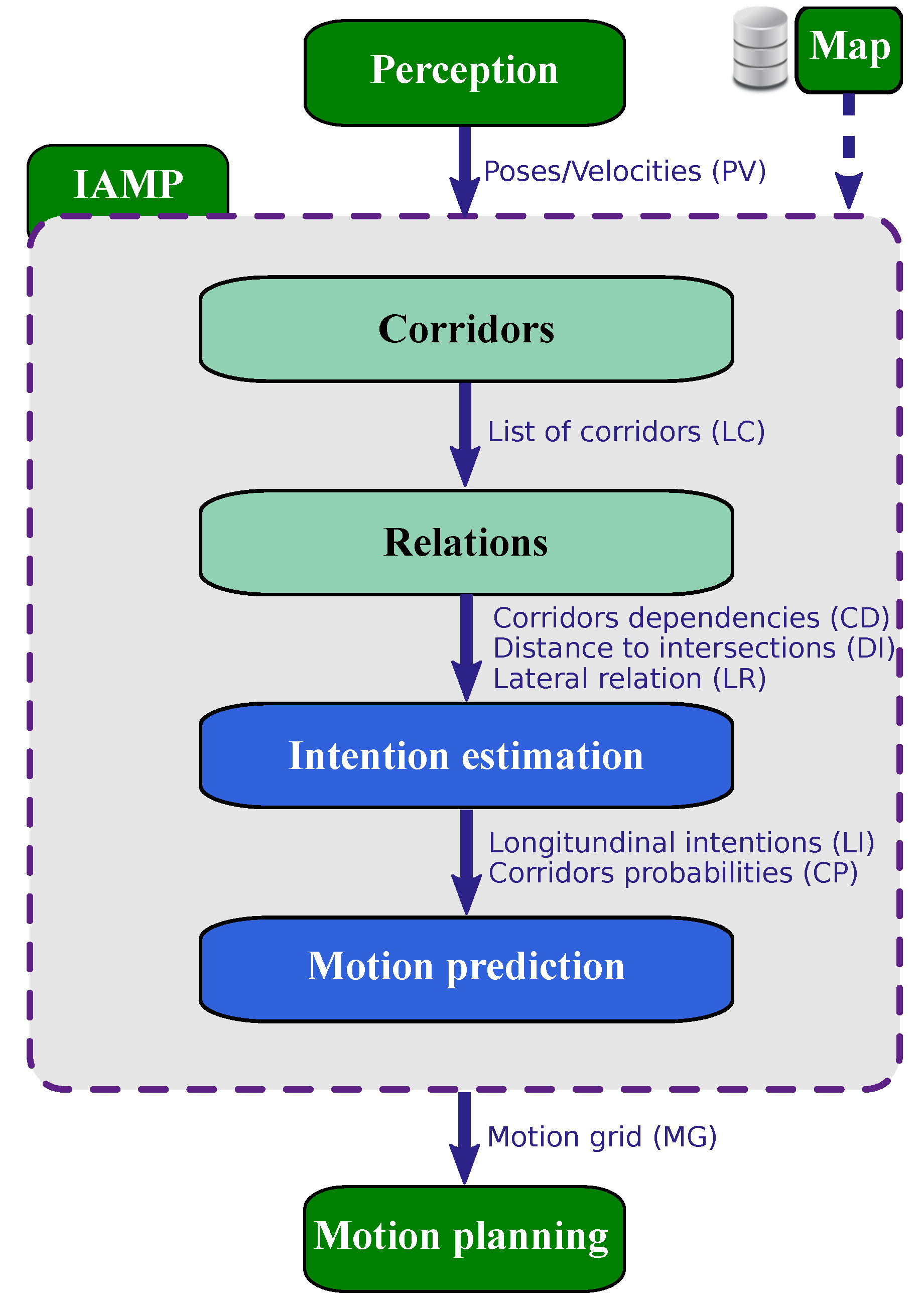
3. Architecture Overview
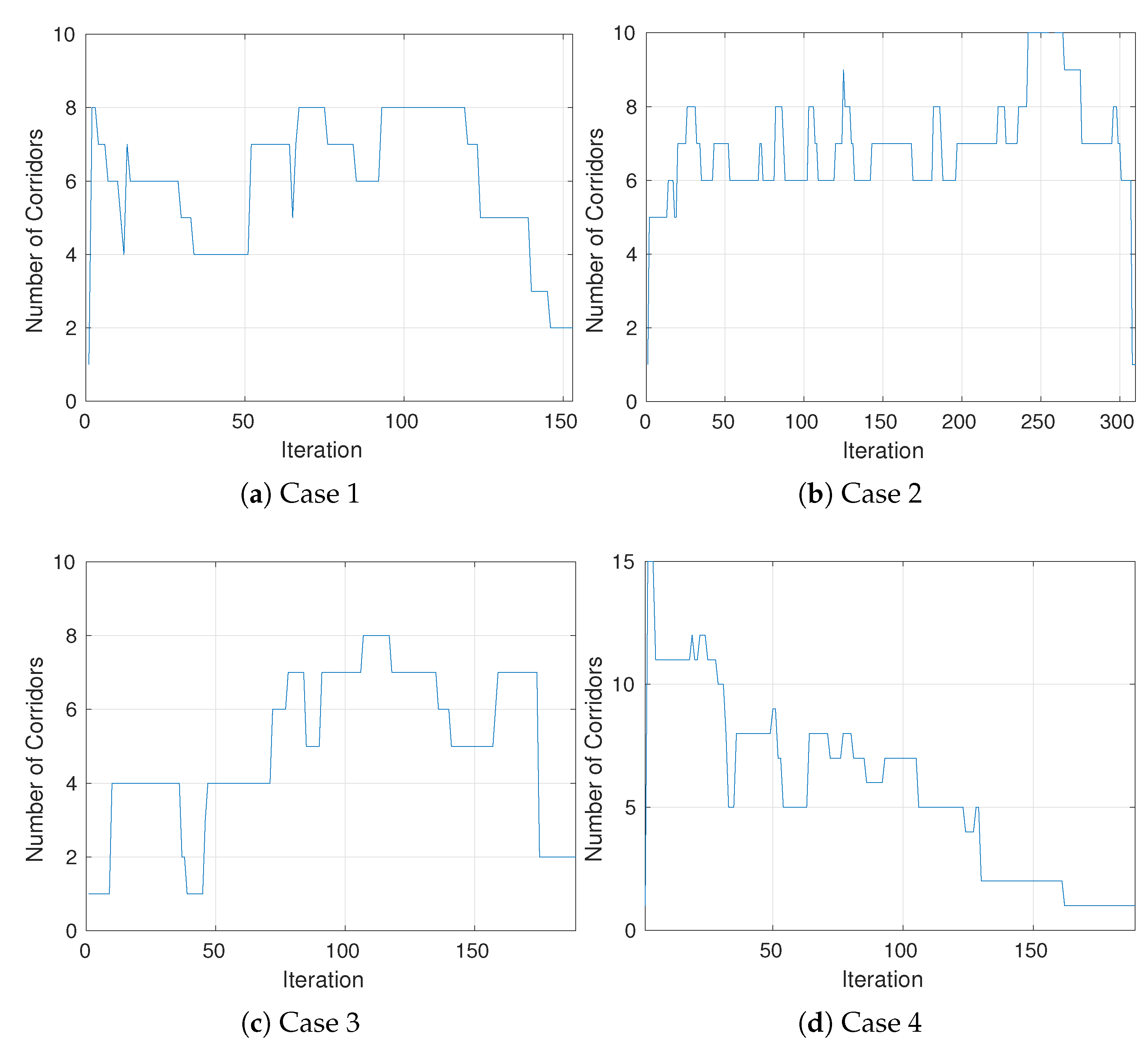
3.1. Corridors
3.2. Relations
- Lateral relation: For each target vehicle, a search of the surrounding vehicles is performed, and the bumper-to-bumper distance and their velocities are stored.
- Corridor-to-intersection: The intersections each corridor goes through are determined by intersecting the lanelet’s identifiers. Then, for all intersections a corridor goes through, the distance to the intersection is computed in the Frenet frame.
- Corridor-to-corridor: In order to determine which corridor will influence the predictions of the other, a search is performed by pairwise intersecting the centerlines of all corridors. This generates a list of possible collisions. Based on a set of rules, one (if any) corridor is selected as the corridor influencing the motion of another vehicle.
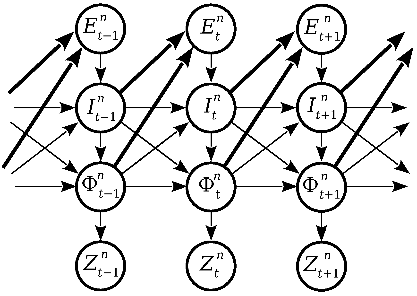
3.3. Intention Estimation
- Expectation : This describes the expected maneuver of a vehicle n at time t based on the road geometry, traffic regulation and other vehicles behavior. It is decomposed in two dimensions: longitudinal and lateral. Longitudinal Expectation, also called Expectation to Stop (), estimates the probability of a vehicle stopping at an intersection. Lateral Expectation, also called Expectation to Change (), estimates the probability of a vehicle changing lanes. Both values are binary, their possible values are go and stop for and stay and change for .
- Intention : This describes the intended maneuver of a vehicle n at time t based on the previous intention, current expectation and vehicle physical state. There are also Lateral and Longitudinal intentions ( and , respectively).
- Physical vehicle state : This describes the estimated position, orientation and speed of each vehicle.
- Measured vehicle state : This describes the measured pose, orientation and speed of each vehicle. They are obtained through the available sensors of the vehicle.
3.4. Motion Prediction
4. Real-Time Framework
4.1. GPU Programming Model
- Global memory is accessible from all threads in the GPU and is the highest in size but it also has the most access latency.
- Shared memory is accessed from within the streaming multiprocessors, is shared across the threads in a block, and has very low latency.
- Local memory is the memory that each thread can statically allocate and is only visible from within the thread.
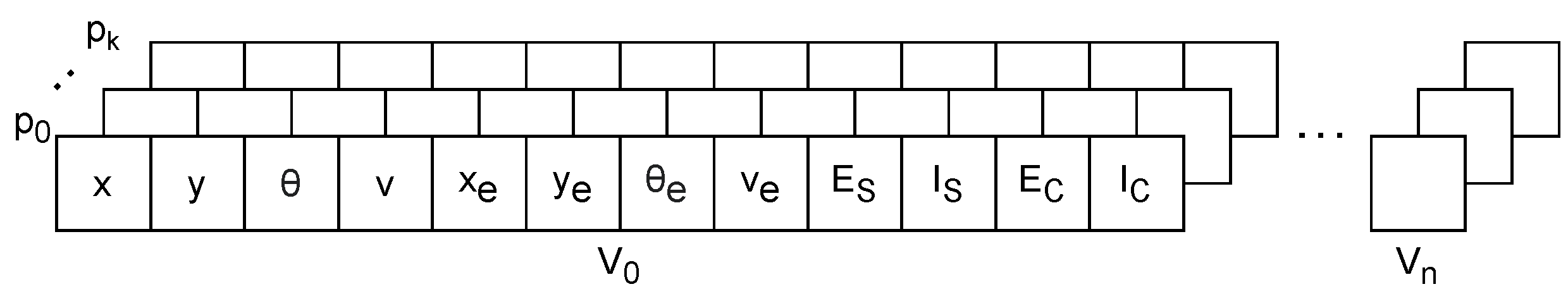
4.2. Parallel Particle Filter
4.2.1. Predict
4.2.2. Update
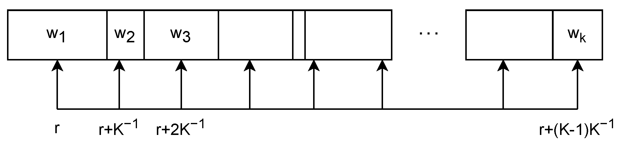
4.2.3. Resample
4.2.4. Output Generation
4.3. Parallel Motion Prediction
4.3.1. Memory-Aligned Matrix Combination
5. Experiments
5.1. Experimental Setup
5.1.1. inD and openDD
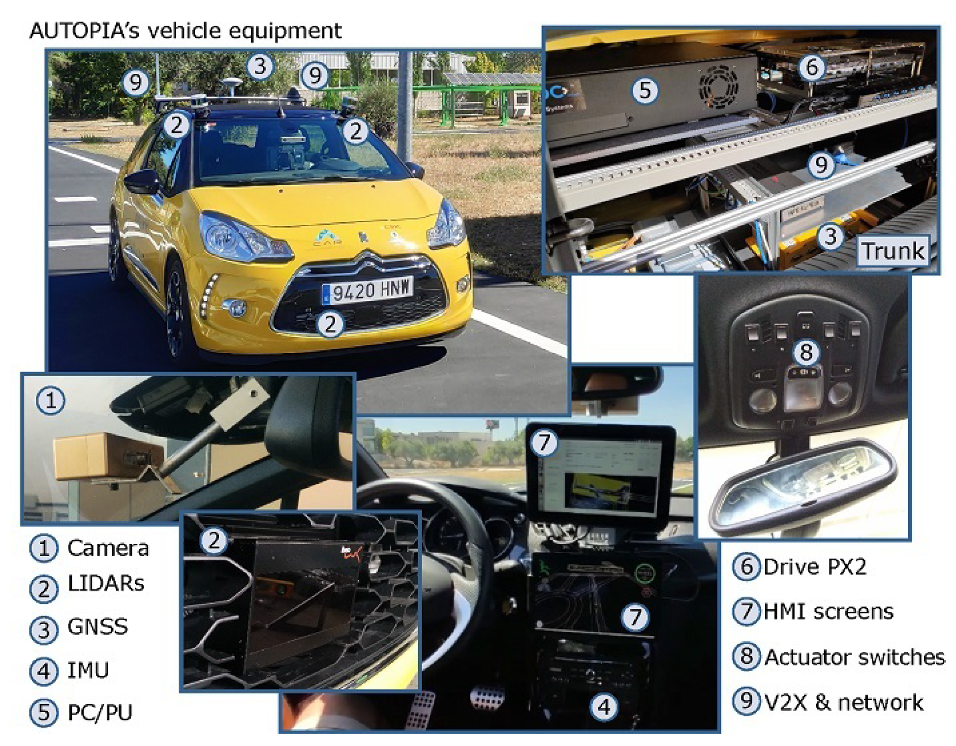
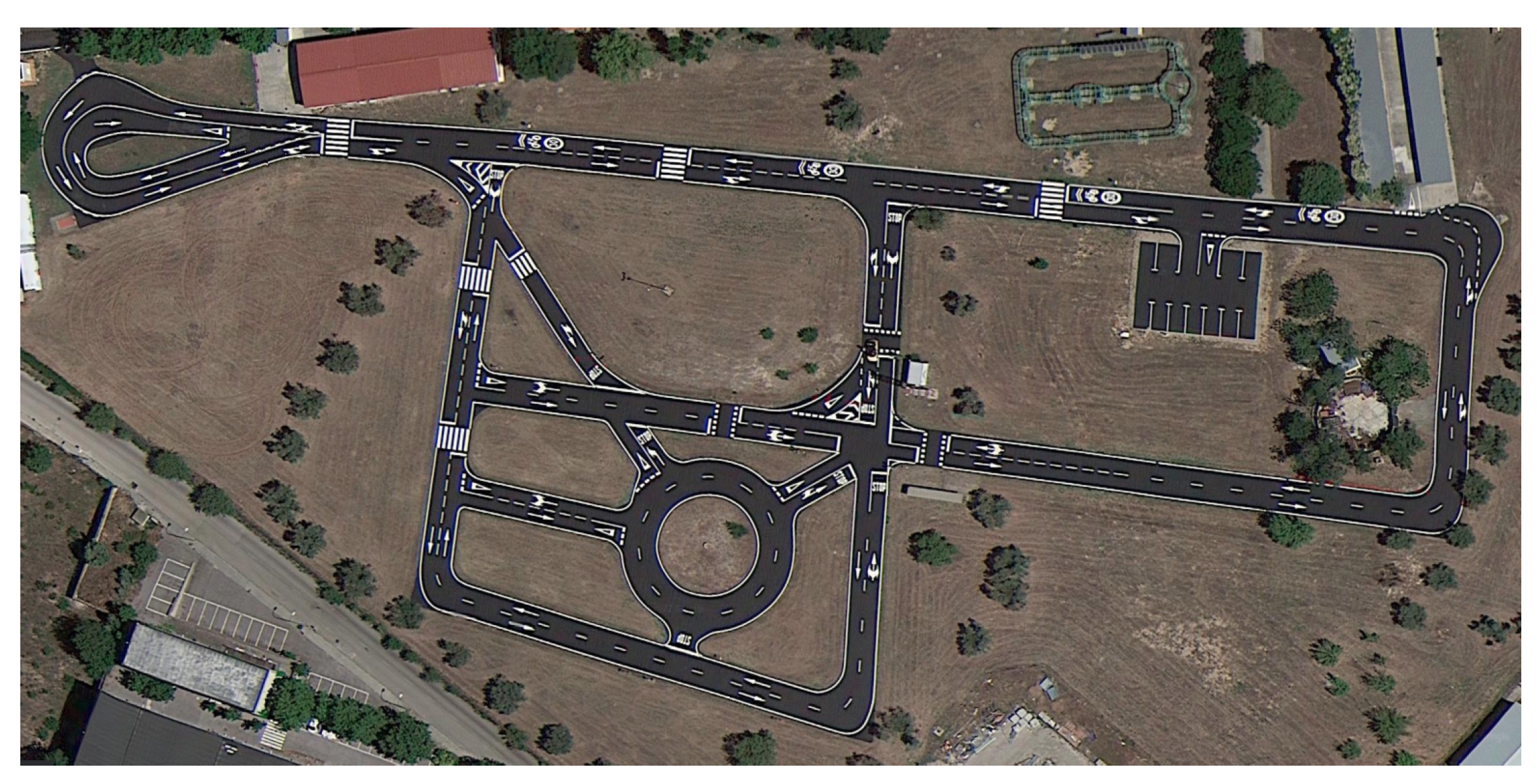
5.1.2. Autopia Test Track
5.1.3. Timing Computation
5.2. Particle Filter
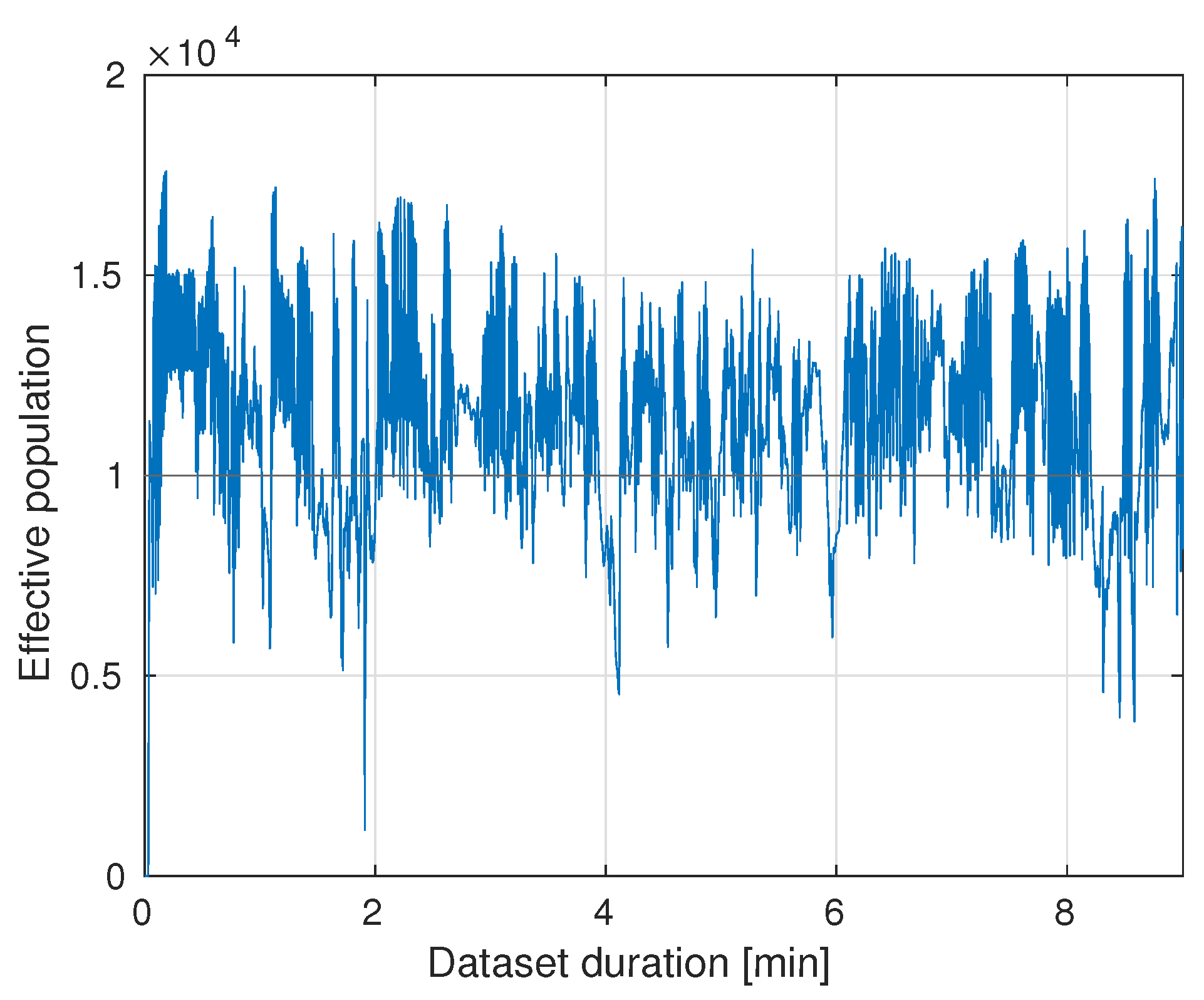
5.2.1. Effective Population
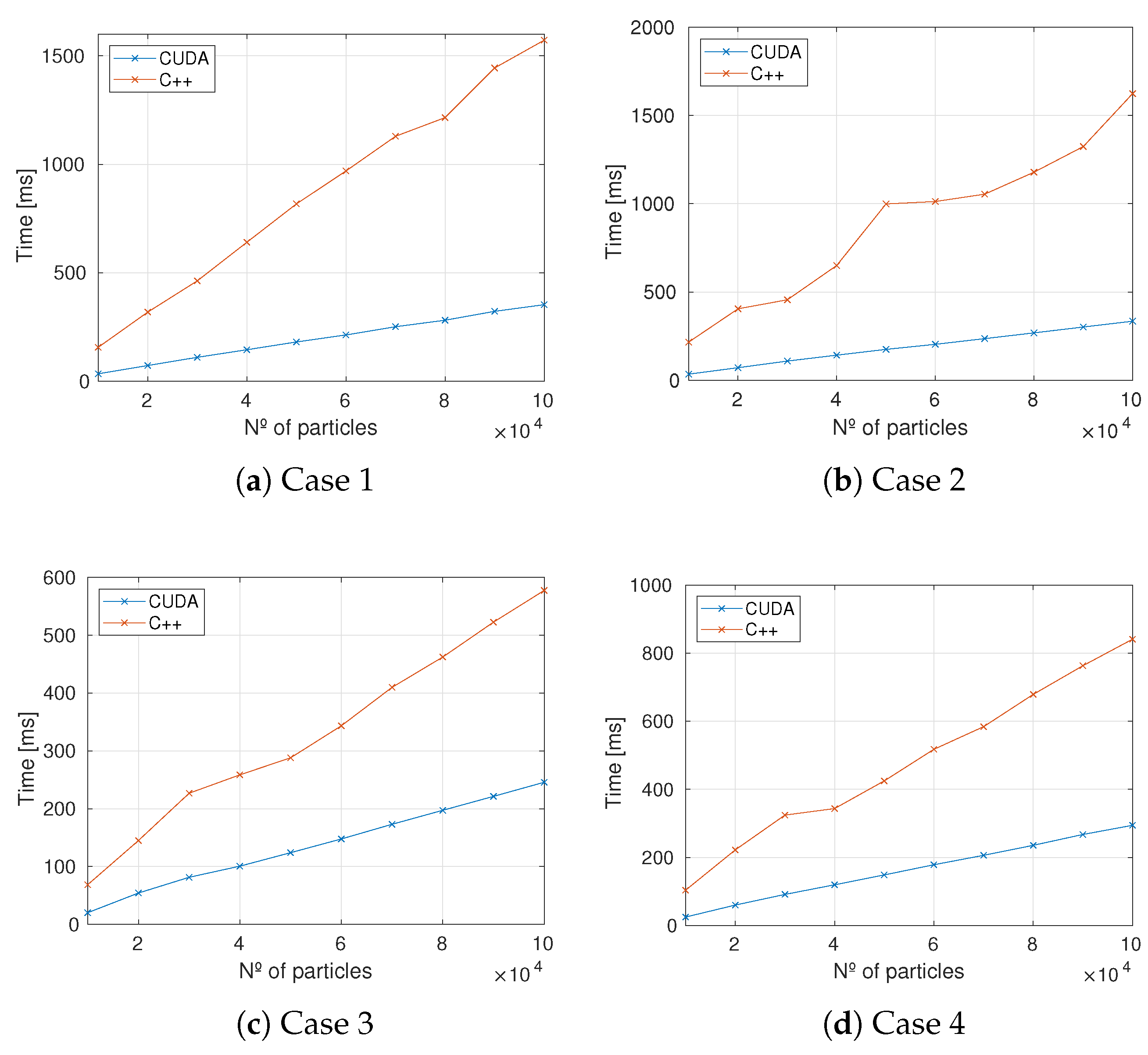
5.2.2. Scalability
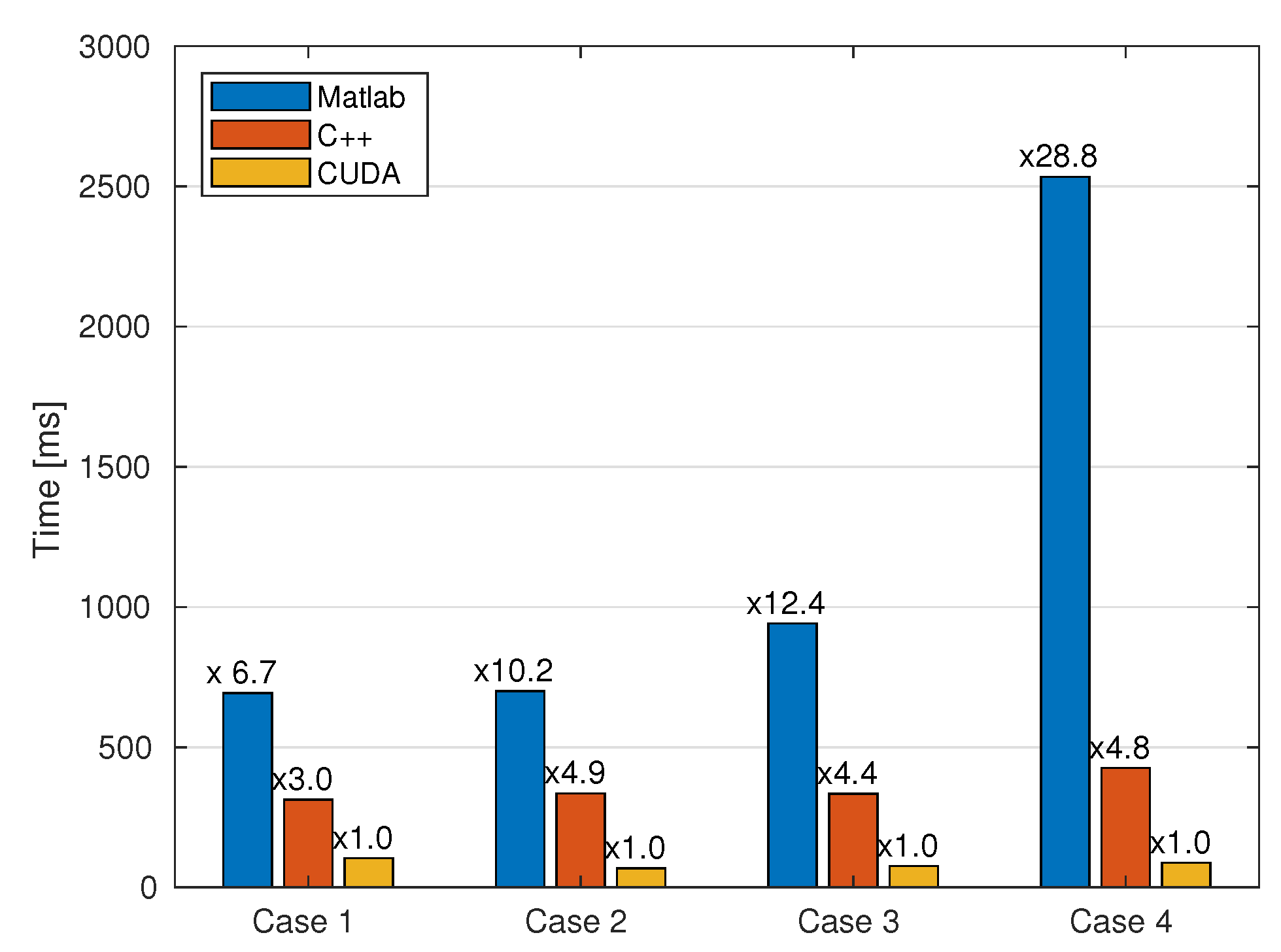
5.3. Motion Prediction
5.4. Complete Loop
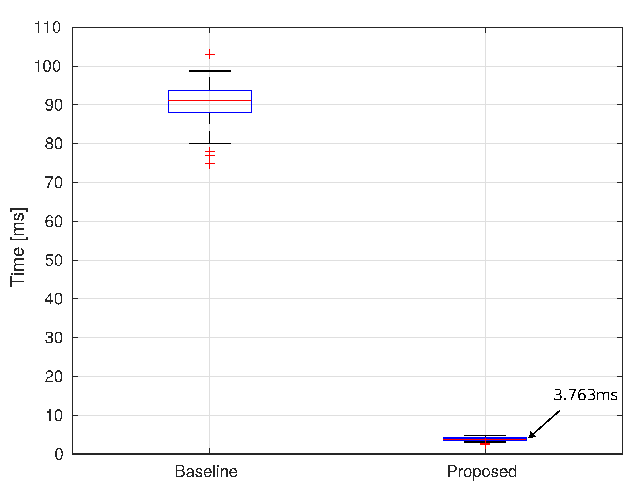
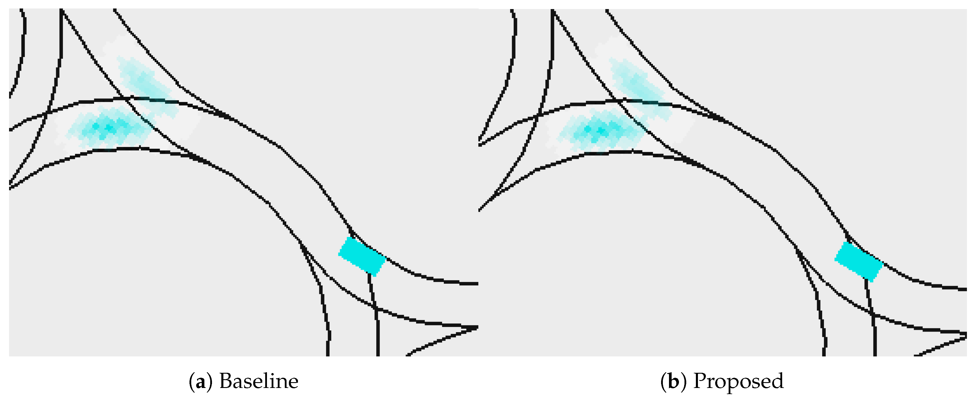
5.5. Baseline Comparison
5.6. Nvidia Drive PX2 Tests
6. Prediction Evaluation
- ADE (average displacement error): average distance between the ground truth positions and the weighted average position of the predictions,
- FDE (final displacement error): distance between the last ground truth position and the weighted average position of the last prediction,
7. Conclusions
Supplementary Materials
Author Contributions
Funding
Institutional Review Board Statement
Informed Consent Statement
Data Availability Statement
Conflicts of Interest
References
- Wang, J.S.; Knipling, R.R.; Goodman, M.J. The role of driver inattention in crashes: New statistics from the 1995 Crashworthiness Data System. In Proceedings of the 40th Annual Proceedings of the Association for the Advancement of Automotive Medicine, Vancouver, BC, Canada, 7–9 October 1996; Volume 377, p. 392. [Google Scholar]
- Rathery, A. Traffic flow problems in Europe. Transp. Rev. 1993, 13, 1–23. [Google Scholar] [CrossRef]
- Berg, J.; Ihlström, J. The importance of public transport for mobility and everyday activities among rural residents. Soc. Sci. 2019, 8, 58. [Google Scholar] [CrossRef]
- Large, R.O.; Breitling, T.; Kramer, N. Driver Shortage and Fluctuation: Occupational and Organizational Commitment of Truck Drivers. Supply Chain Forum Int. J. 2014, 15, 66–72. [Google Scholar] [CrossRef]
- Villagra, J.; Clavijo, M.; Díaz-Álvarez, A.; Trentin, V. Motion prediction and risk assessment. In Decision-Making Techniques for Autonomous Vehicles; Elsevier: Amsterdam, The Netherlands, 2023; pp. 61–101. [Google Scholar]
- Gerlein, E.A.; Díaz-Guevara, G.; Carrillo, H.; Parra, C.; Gonzalez, E. Embbedded system-on-chip 3D localization and mapping—eSoC-SLAM. Electronics 2021, 10, 1378. [Google Scholar] [CrossRef]
- Hao, C.; Sarwari, A.; Jin, Z.; Abu-Haimed, H.; Sew, D.; Li, Y.; Liu, X.; Wu, B.; Fu, D.; Gu, J.; et al. A hybrid GPU+ FPGA system design for autonomous driving cars. In Proceedings of the 2019 IEEE International Workshop on Signal Processing Systems (SiPS), Nanjing, China, 20–23 October 2019; IEEE: Piscataway, NJ, USA, 2019; pp. 121–126. [Google Scholar]
- Nadales, J.; Manzano, J.; Barriga, A.; Limon, D. Efficient FPGA Parallelization of Lipschitz Interpolation for Real-Time Decision-Making. IEEE Trans. Control Syst. Technol. 2022, 30, 2163–2175. [Google Scholar] [CrossRef]
- Haneche, A.; Lachachi, Y.; Niar, S.; Ouarnoughi, H. A GPU enhanced LIDAR Perception System for Autonomous Vehicles. In Proceedings of the 2020 28th Euromicro International Conference on Parallel, Distributed and Network-Based Processing (PDP), Västerås, Sweden, 11–13 March 2020; IEEE: Piscataway, NJ, USA, 2020; pp. 232–236. [Google Scholar]
- Xie, X.; Bai, L.; Huang, X. Real-time LiDAR point cloud semantic segmentation for autonomous driving. Electronics 2021, 11, 11. [Google Scholar] [CrossRef]
- Shah, H.; Ghadai, S.; Gamdha, D.; Schuster, A.; Thomas, I.; Greiner, N.; Krishnamurthy, A. GPU-Accelerated Collision Analysis of Vehicles in a Point Cloud Environment. IEEE Comput. Graph. Appl. 2022, 42, 37–50. [Google Scholar] [CrossRef] [PubMed]
- Mufti, S.; Roberge, V.; Tarbouchi, M. A GPU accelerated path planner for multiple unmanned aerial vehicles. In Proceedings of the 2019 IEEE Canadian Conference of Electrical and Computer Engineering (CCECE), Edmonton, AB, Canada, 5–8 May 2019; IEEE: Piscataway, NJ, USA, 2019; pp. 1–4. [Google Scholar]
- Chen, Z.; Khemmar, R.; Decoux, B.; Atahouet, A.; Ertaud, J.Y. Real time object detection, tracking, and distance and motion estimation based on deep learning: Application to smart mobility. In Proceedings of the 2019 Eighth International Conference on Emerging Security Technologies (EST), Colchester, UK, 22–24 July 2019; IEEE: Piscataway, NJ, USA, 2019; pp. 1–6. [Google Scholar]
- Nicely, M.A.; Wells, B.E. Improved parallel resampling methods for particle filtering. IEEE Access 2019, 7, 47593–47604. [Google Scholar] [CrossRef]
- Chen, X.; Sun, L. Bayesian temporal factorization for multidimensional time series prediction. IEEE Trans. Pattern Anal. Mach. Intell. 2021, 44, 4659–4673. [Google Scholar] [CrossRef]
- Wang, P.; Zhang, Y.; Hu, T.; Zhang, T. Urban traffic flow prediction: A dynamic temporal graph network considering missing values. Int. J. Geogr. Inf. Sci. 2023, 37, 885–912. [Google Scholar] [CrossRef]
- Althoff, M.; Mergel, A. Comparison of Markov chain abstraction and Monte Carlo simulation for the safety assessment of autonomous cars. IEEE Trans. Intell. Transp. Syst. 2011, 12, 1237–1247. [Google Scholar] [CrossRef]
- Hubmann, C.; Becker, M.; Althoff, D.; Lenz, D.; Stiller, C. Decision making for autonomous driving considering interaction and uncertain prediction of surrounding vehicles. In Proceedings of the 2017 IEEE Intelligent Vehicles Symposium (IV), Los Angeles, CA, USA, 11–14 June 2017; IEEE: Piscataway, NJ, USA, 2017; pp. 1671–1678. [Google Scholar]
- Poggenhans, F.; Pauls, J.H.; Janosovits, J.; Orf, S.; Naumann, M.; Kuhnt, F.; Mayr, M. Lanelet2: A High-Definition Map Framework for the Future of Automated Driving. In Proceedings of the 2018 21st International Conference on Intelligent Transportation Systems (ITSC), Maui, HI, USA, 4–7 November 2018; pp. 1672–1679. [Google Scholar]
- Trentin, V.; Artuñedo, A.; Godoy, J.; Villagra, J. Multi-Modal Interaction-Aware Motion Prediction At Unsignalized Intersections. IEEE Trans. Intell. Veh. 2023, 1–17. [Google Scholar] [CrossRef]
- Trentin, V.; Artuñedo, A.; Godoy, J.; Villagra, J. Interaction-Aware Motion Prediction at Highways: A Comparison of Three Lane Changing Models. In Proceedings of the Smart Cities, Green Technologies, and Intelligent Transport Systems; Klein, C., Jarke, M., Helfert, M., Berns, K., Gusikhin, O., Eds.; Springer: Cham, Switzerland, 2022; pp. 274–296. [Google Scholar]
- Trentin, V.; Artuñedo, A.; Godoy, J.; Villagra, J. Interaction-Aware Intention Estimation at Roundabouts. IEEE Access 2021, 9, 123088–123102. [Google Scholar] [CrossRef]
- Lefèvre, S.; Laugier, C.; Ibañez-Guzmán, J. Intention-Aware Risk Estimation for General Traffic Situations, and Application to Intersection Safety; Research Report RR-8379; INRIA, Hal: Le Chesnay-Rocquencourt, France, 2013. [Google Scholar]
- Derks, I.P.; de Waal, A. A Taxonomy of Explainable Bayesian Networks. In Proceedings of the Artificial Intelligence Research; Gerber, A., Ed.; Springer: Cham, Switzerland, 2020; pp. 220–235. [Google Scholar]
- Arulampalam, M.S.; Maskell, S.; Gordon, N.; Clapp, T. A tutorial on particle filters for online nonlinear/non-Gaussian Bayesian tracking. IEEE Trans. Signal Process. 2002, 50, 174–188. [Google Scholar] [CrossRef]
- Althoff, M. Reachability Analysis and its Application to the Safety Assessment of Autonomous Cars. Ph.D. Thesis, Technische Universität München, Munchen, Germany, 2010. [Google Scholar]
- NVIDIA. CUDA API Documentation. Available online: https://docs.nvidia.com/cuda/cuda-runtime-api/index.html (accessed on 30 June 2022).
- NVIDIA. CUDA C Programming Guide. Available online: https://docs.nvidia.com/cuda/cuda-c-programming-guide (accessed on 24 May 2022).
- Gil, A.; Segura, J.; Temme, N. Numerical Methods for Special Functions; SIAM: Philadelphia, PA, USA, 2007; pp. 193–197. [Google Scholar]
- Li, T.; Bolic, M.; Djuric, P.M. Resampling methods for particle filtering: Classification, implementation, and strategies. IEEE Signal Process. Mag. 2015, 32, 70–86. [Google Scholar] [CrossRef]
- Thrun, S.; Burgard, W.; Fox, D. Probabilistic Robotics (Intelligent Robotics and Autonomous Agents); The MIT Press: Cambridge, MA, USA, 2005. [Google Scholar]
- Cano, A.; Zafra, A.; Ventura, S. Parallel evaluation of Pittsburgh rule-based classifiers on GPUs. Neurocomputing 2014, 126, 45–57. [Google Scholar] [CrossRef][Green Version]
- Bock, J.; Krajewski, R.; Moers, T.; Runde, S.; Vater, L.; Eckstein, L. The inD Dataset: A Drone Dataset of Naturalistic Road User Trajectories at German Intersections. In Proceedings of the 2020 IEEE Intelligent Vehicles Symposium (IV), Las Vegas, NV, USA, 19 October–13 November 2020; pp. 1929–1934. [Google Scholar] [CrossRef]
- Breuer, A.; Termöhlen, J.A.; Homoceanu, S.; Fingscheidt, T. openDD: A large-scale roundabout drone dataset. In Proceedings of the 2020 IEEE 23rd International Conference on Intelligent Transportation Systems (ITSC), Rhodes, Greece, 20–23 September 2020; IEEE: Piscataway, NJ, USA, 2020; pp. 1–6. [Google Scholar]
- AUTOPIA. CAR CSIC. Available online: https://autopia.car.upm-csic.es/ (accessed on 30 June 2022).
- MATLAB. TIC/TOC Timing Framework. Available online: https://es.mathworks.com/help/matlab/ref/tic.html?lang=en (accessed on 16 April 2023).
- Linux. gettimeofday—Linux Manual Page. Available online: https://man7.org/linux/man-pages/man2/gettimeofday.2.html (accessed on 16 April 2023).
- MATLAB. Creating More Accurate Time Values. Available online: https://es.mathworks.com/company/newsletters/articles/improvements-to-tic-and-toc-functions-for-measuring-absolute-elapsed-time-performance-in-matlab.html (accessed on 16 April 2023).
- STD. steady_clock—Chrono Manual Page. Available online: https://en.cppreference.com/w/cpp/chrono/steady_clock (accessed on 16 April 2023).
- Linux. clock_gettime—Linux Manual Page. Available online: https://linux.die.net/man/3/clock_gettime (accessed on 16 April 2023).
- NVIDIA. CUDA Event Manual Page. Available online: https://docs.nvidia.com/cuda/cuda-runtime-api/group__CUDART__EVENT.html (accessed on 16 April 2023).
- Artunedo, A.; Villagra, J.; Godoy, J. Real-time motion planning approach for automated driving in urban environments. IEEE Access 2019, 7, 180039–180053. [Google Scholar] [CrossRef]
- Medina-Lee, J.; Artuñedo, A.; Godoy, J.; Villagra, J. Merit-Based Motion Planning for Autonomous Vehicles in Urban Scenarios. Sensors 2021, 21, 3755. [Google Scholar] [CrossRef]
- Thrust. Permutation Iterator Documentation. Available online: https://thrust.github.io/doc/classthrust_1_1permutation__iterator.html (accessed on 15 April 2023).
- Thrust. Parallel Copy Documentation. Available online: https://thrust.github.io/doc/group__copying_ga3e43fb8472db501412452fa27b931ee2.html (accessed on 15 April 2023).
- Thrust. The C++ Parallel Algorithms Library. Available online: https://github.com/NVIDIA/thrust (accessed on 15 April 2023).
- NVIDIA. CUDA Programming Guide. Available online: https://docs.nvidia.com/cuda/archive/9.2/cuda-c-programming-guide/index.html#atomicadd (accessed on 15 May 2023).
- NVIDIA. cuSPARSE Documentation. Available online: https://docs.nvidia.com/cuda/archive/9.2/cusparse/index.html#cusparse-lt-t-gt-csrgemm (accessed on 10 April 2022).
- Jiménez, V.; Godoy, J.; Artuñedo, A.; Villagra, J. Object-level Semantic and Velocity Feedback for Dynamic Occupancy Grids. IEEE Trans. Intell. Veh. 2023, 8, 1–18. [Google Scholar] [CrossRef]
- Godoy, J.; Jiménez, V.; Artuñedo, A.; Villagra, J. A grid-based framework for collective perception in autonomous vehicles. Sensors 2021, 21, 744. [Google Scholar] [CrossRef]
- Li, X.; Ying, X.; Chuah, M.C. Grip++: Enhanced graph-based interaction-aware trajectory prediction for autonomous driving. arXiv 2019, arXiv:1907.07792. [Google Scholar]
- Trentin, V.; Ma, C.; Villagra, J.; Al-Ars, Z. Learning-enabled multi-modal motion prediction in urban environments. In Proceedings of the 2023 IEEE Intelligent Vehicles Symposium (IV), Dearborn, MI, USA, 4–7 June 2023; pp. 1–7. [Google Scholar]


| Implementation | Case 1 | Case 2 | Case 3 | Case 4 |
|---|---|---|---|---|
| C++ | 0.068 | 0.137 | 0.028 | 0.011 |
| CUDA | 0.152 | 0.250 | 0.174 | 0.135 |
| Scenario | Matlab | C++ | CUDA |
|---|---|---|---|
| Case 1 | 24.536× | 4.841× | 1× |
| Case 2 | 41.280× | 4.570× | 1× |
| Case 3 | 57.341× | 4.664× | 1× |
| Case 4 | 115.098× | 6.131× | 1× |
| Scenario | Matlab [Hz] | C++ [Hz] | CUDA [Hz] |
|---|---|---|---|
| Case 1 | 0.199 | 1.013 | 4.906 |
| Case 2 | 0.207 | 1.870 | 8.549 |
| Case 3 | 0.105 | 1.300 | 6.065 |
| Case 4 | 0.050 | 1.938 | 5.755 |
| Approach | Metric | Case 1 | Case 2 | Case 3 | Case 4 |
|---|---|---|---|---|---|
| IAMP | ADE | 1.08 | 1.13 | 1.53 | 1.84 |
| FDE | 2.42 | 2.80 | 4.20 | 4.98 | |
| GRIP | ADE | 1.82 | 2.38 | 4.81 | 3.95 |
| FDE | 4.63 | 6.06 | 12.18 | 10.31 |
| Scenario | IAMP [ms] | GRIP [ms] |
|---|---|---|
| Case 1 | 103 | 65 |
| Case 2 | 68 | 65 |
| Case 3 | 76 | 64 |
| Case 4 | 87 | 68 |
Disclaimer/Publisher’s Note: The statements, opinions and data contained in all publications are solely those of the individual author(s) and contributor(s) and not of MDPI and/or the editor(s). MDPI and/or the editor(s) disclaim responsibility for any injury to people or property resulting from any ideas, methods, instructions or products referred to in the content. |
© 2023 by the authors. Licensee MDPI, Basel, Switzerland. This article is an open access article distributed under the terms and conditions of the Creative Commons Attribution (CC BY) license (https://creativecommons.org/licenses/by/4.0/).
Share and Cite
Hortelano, J.L.; Trentin, V.; Artuñedo, A.; Villagra, J. GPU-Accelerated Interaction-Aware Motion Prediction. Electronics 2023, 12, 3751. https://doi.org/10.3390/electronics12183751
Hortelano JL, Trentin V, Artuñedo A, Villagra J. GPU-Accelerated Interaction-Aware Motion Prediction. Electronics. 2023; 12(18):3751. https://doi.org/10.3390/electronics12183751
Chicago/Turabian StyleHortelano, Juan Luis, Vinicius Trentin, Antonio Artuñedo, and Jorge Villagra. 2023. "GPU-Accelerated Interaction-Aware Motion Prediction" Electronics 12, no. 18: 3751. https://doi.org/10.3390/electronics12183751
APA StyleHortelano, J. L., Trentin, V., Artuñedo, A., & Villagra, J. (2023). GPU-Accelerated Interaction-Aware Motion Prediction. Electronics, 12(18), 3751. https://doi.org/10.3390/electronics12183751