Investigation of the Feasibility of the Dynamic Equivalent Model of Large Photovoltaic Power Plants in a Harmonic Resonance Study

Abstract

In recent years, there have been several harmonic resonance accidents around the world that involve renewable energy power plants. The frequency scanning method is the most widely used technique in engineering practice to evaluate the severity of resonance due to its simple operation and clear physical meaning. However, when establishing electromagnetic transient simulation models and conducting frequency scans, a single generation unit or a few renewable generation units are usually used to represent the original power plant for the purpose of reducing model complexity and improving the simulation efficiency. Such a practice has been found to be effective in dynamic studies around the fundamental frequency. However, its feasibility in harmonic resonance studies has not yet been fully investigated. Because of this research gap, a feasibility study is conducted in this paper by using a real-life photovoltaic power plant. The detailed harmonic model of the plant is first established using the harmonic linearization method, and the equivalent harmonic model is then developed using the power loss conservation method. The feasibility of the equivalent model was investigated in detail, and the impact of the different impedance models on the resonance analysis was analyzed. The results indicate that the conventional dynamic equivalent model can effectively reflect the harmonic resonance characteristics of photovoltaic power plants. Furthermore, a more simplified model that ignores the inductance of the collector line is recommended in this paper to further reduce the modeling complexity.

1. Introduction

With the increasing prominence of environmental issues, the development of renewable energy power plants, such as solar power plants, has rapidly progressed; moreover, renewable energy power plants have become an important supporting power source for power systems around the world [1,2]. However, in the grid integration practice of large-scale renewable energy power plants, several harmonic resonance accidents have occurred, as shown in Table 1. This resonance phenomenon involves the interaction of various voltage-source inverters, transmission networks, and other power electronic devices [3], exhibiting strong harmonic coupling [4] and a wide resonance frequency range [5]. In severe situations, it may even cause the system to lose its stability [6], posing a threat to the safe and reliable operation of the system.

Table 1. Harmonic resonance events that occur in actual power systems.

References	Spot	Resonant Frequency/Hz	Possible Cause of Resonance
[7]	Offshore wind farms in Denmark (Horns Rev)	300–350, 750–800	Filters, Submarine Cables
[8]	A 49 MW photovoltaic power station in Yueyang City	1050–1200	Filter
[9]	A photovoltaic power station in Huyanghe City	2500	Static Synchronous Compensator
[10]	Offshore wind farms in Germany (BorWin1)	250–300	Voltage Source Converter
[11]	A 50 MW photovoltaic power station in Qinghai Province	1050–1350	Voltage Source Converter
[12]	A wind farm in Guangdong province	650	Filter
[13]	A wind farm in Guangdong province	3–12	weak grid

Table 1. Harmonic resonance events that occur in actual power systems.

References	Spot	Resonant Frequency/Hz	Possible Cause of Resonance
[7]	Offshore wind farms in Denmark (Horns Rev)	300–350, 750–800	Filters, Submarine Cables
[8]	A 49 MW photovoltaic power station in Yueyang City	1050–1200	Filter
[9]	A photovoltaic power station in Huyanghe City	2500	Static Synchronous Compensator
[10]	Offshore wind farms in Germany (BorWin1)	250–300	Voltage Source Converter
[11]	A 50 MW photovoltaic power station in Qinghai Province	1050–1350	Voltage Source Converter
[12]	A wind farm in Guangdong province	650	Filter
[13]	A wind farm in Guangdong province	3–12	weak grid

Currently, the commonly used methods for harmonic resonance analysis include eigenvalue analysis [14], impedance analysis [15], and frequency scan analysis [16]. Due to its simplicity and clear physical interpretation, frequency scan analysis has been widely applied in engineering practices [17]. Reference [18] used frequency scan analysis to reveal the sub-synchronous control interaction between the control loop of doubly fed induction generators and series capacitor compensation in the power system. They further discussed the influence mechanism of the control parameters on the system impedance and resonance frequency. Reference [19] utilized frequency scan analysis to plot the impedance curve of doubly fed wind turbines to explore their high-frequency resonance characteristics in the grid connection. Notably, references [18,19] did not use detailed electromagnetic transient models in their frequency scan analysis of large-scale renewable energy power plants but instead employed aggregated dynamic equivalent models to reduce the model complexity.

In fact, using a single generation unit or a few units to represent a large-scale renewable energy power plant is a popular approach for electromagnetic transient simulations and related analysis. References [13,20,21,22] ignored the collector lines between photovoltaic/wind generation units and analyzed photovoltaic/wind power plants using an equivalent photovoltaic/wind turbine unit. Reference [23] studied the equivalent method of photovoltaic arrays, transformers, and collector lines for the equivalent model of a large-scale photovoltaic (PV) power plant. They validated the proposed method using a 100 MW real-life PV power plant in northern Chile. References [24,25] used the equal voltage loss method to obtain the parameters of the collector lines in the single-unit equivalent model, considering different topological structures in wind farms. Reference [26] used the power loss conservation method to obtain the equivalent impedance model of a wind farm. Notably, the dynamic equivalent models established in the aforementioned references are only demonstrated for transient studies or oscillation issues near the fundamental frequency. However, the feasibility of the equivalent method in the harmonic frequency range still needs to be investigated. The result is very important for determining whether the frequency scan result of a single equivalent unit can be used for harmonic resonance analysis with confidence.

Therefore, in this paper, a large-scale PV power plant is taken as an example, an accurate impedance model is established using a bottom-up modeling method, and a dynamic equivalent model is established using the power loss conservation method. The differences between the equivalent model and the accurate model in the harmonic frequency range are analyzed in detail. The result indicates that the capacitance of the collector line plays an important role in the harmonic frequency, while the impact of the series impedance of the line is much smaller. Therefore, the collector line can be further simplified as a capacitor, which leads to a more simplified model. The findings provide guidance on the selection of proper models in practical harmonic resonance analysis.

The rest of the paper is organized as follows: In Section 2, the system structure and parameters of the PV plant under study are explained. In Section 3, the accurate impedance model of the PV plant is derived using the bottom-up modeling method. In Section 4, the equivalent impedance model of the PV plant is derived using the power loss conservation method. In Section 5, the accurate model and the equivalent model are used to conduct a harmonic resonance study of a real-life power plant, and the performances of the two methods are compared in detail. Finally, in Section 6, the paper is concluded.

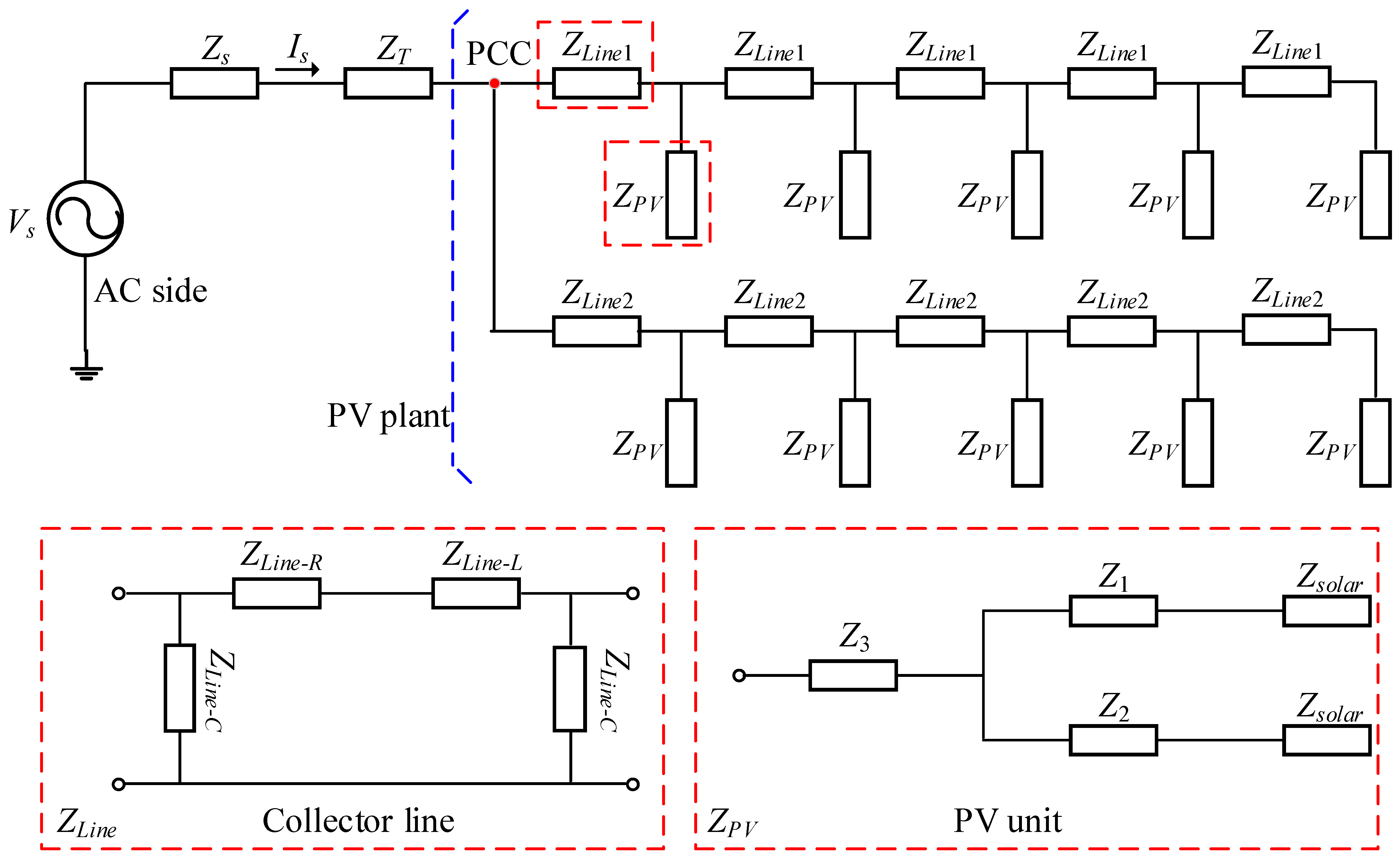
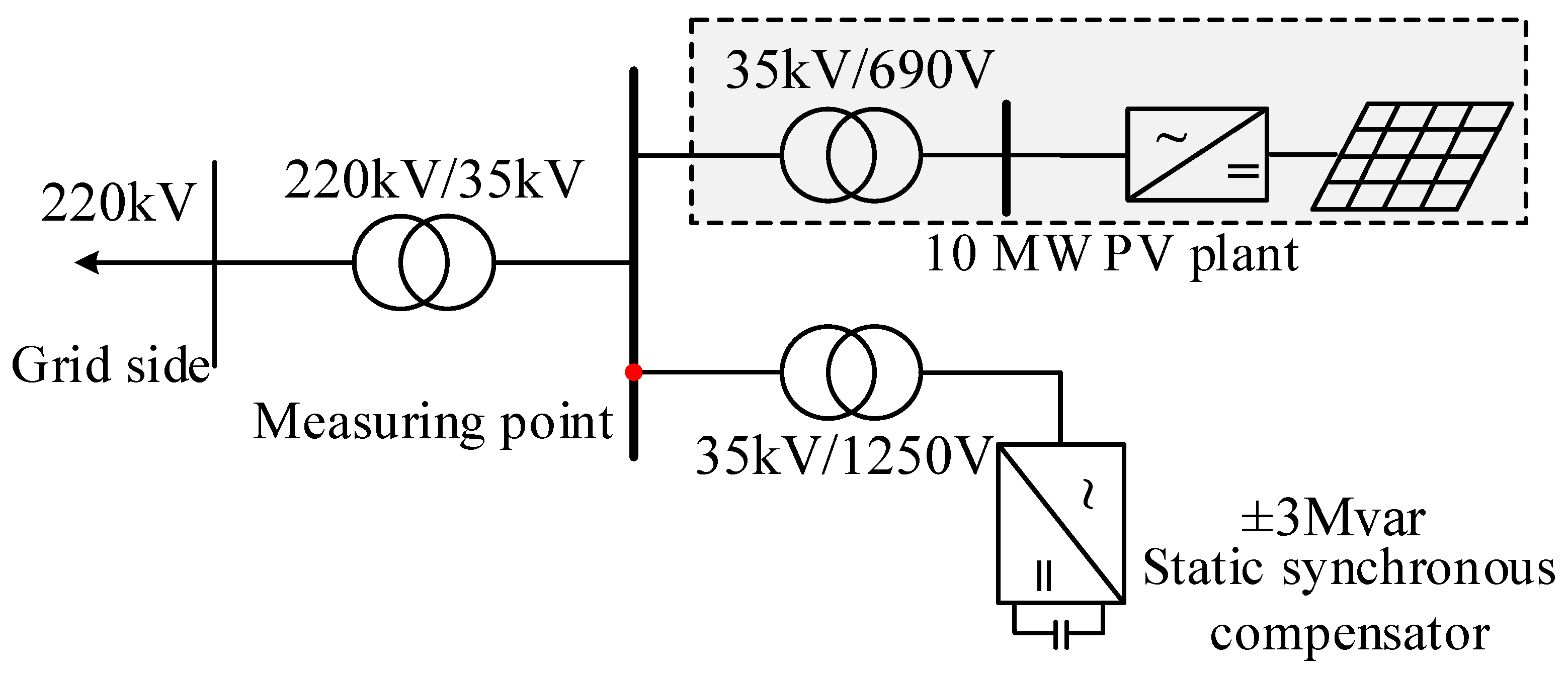
2. System Structure and Parameters of the PV Plant

Figure 1 illustrates the topology structure of a large-scale PV power plant with an installed capacity of 2 × 5 MW. The plant consists of two feeders, with each feeder connecting five 1 MW PV generation units. Each PV generation unit comprises two sets of 0.5 MW grid-connected inverters and a 35 kV/690 V/690 V distribution transformer. The adjacent PV generation units are connected by collector lines, which typically have a cross-sectional area ranging from 3 × 50 mm² to 3 × 300 mm².

The grid-connected inverter adopts a dual-loop control structure, as shown in Figure 2. The power control loop is responsible for regulating the active power (P) and reactive power (Q) to ensure stability and provide reference signals to the current control loop. The current control loop further outputs a modulation signal (m_abc), which is fed into the pulse width modulation (PWM) switch to generate the switching function for the conversion from DC voltage to AC output voltage (V_c). Here, V_g and I_g represent the grid voltage and current at the point of the grid connection, respectively. H_PQ(s) = k_pPQ + k_iPQ/s is the transfer function of the power control loop, while H_i(s) = k_pi + k_ii/s is the transfer function of the internal current control loop. K_i represents the decoupling term.

3. Accurate Impedance Model of the PV Plant

Figure 3 illustrates the process of establishing an accurate impedance model for a large-scale PV plant. First, key variables and parameters of the PV plant, including the solar irradiance, control structure, and parameters of the grid-connected inverters, electrical parameters of the transformers, and impedances of the collector lines, are collected. Next, the steady-state operating parameters of the system, such as the bus voltage and the branch power, are determined using the load flow study. Then, the nonlinear PV plant can be linearized at the steady state. Impedance modeling techniques such as harmonic linearization can be applied to obtain the impedance model of each component. Finally, the impedances of various components in the PV power plant are connected based on the network topology, resulting in a site-level impedance network. When studying harmonic resonance characteristics or harmonic instability issues at the site level, complex impedance networks can be aggregated into a single high-order impedance through network transformation. In the rest of this section, the model of each component in the PV plant will be explained.

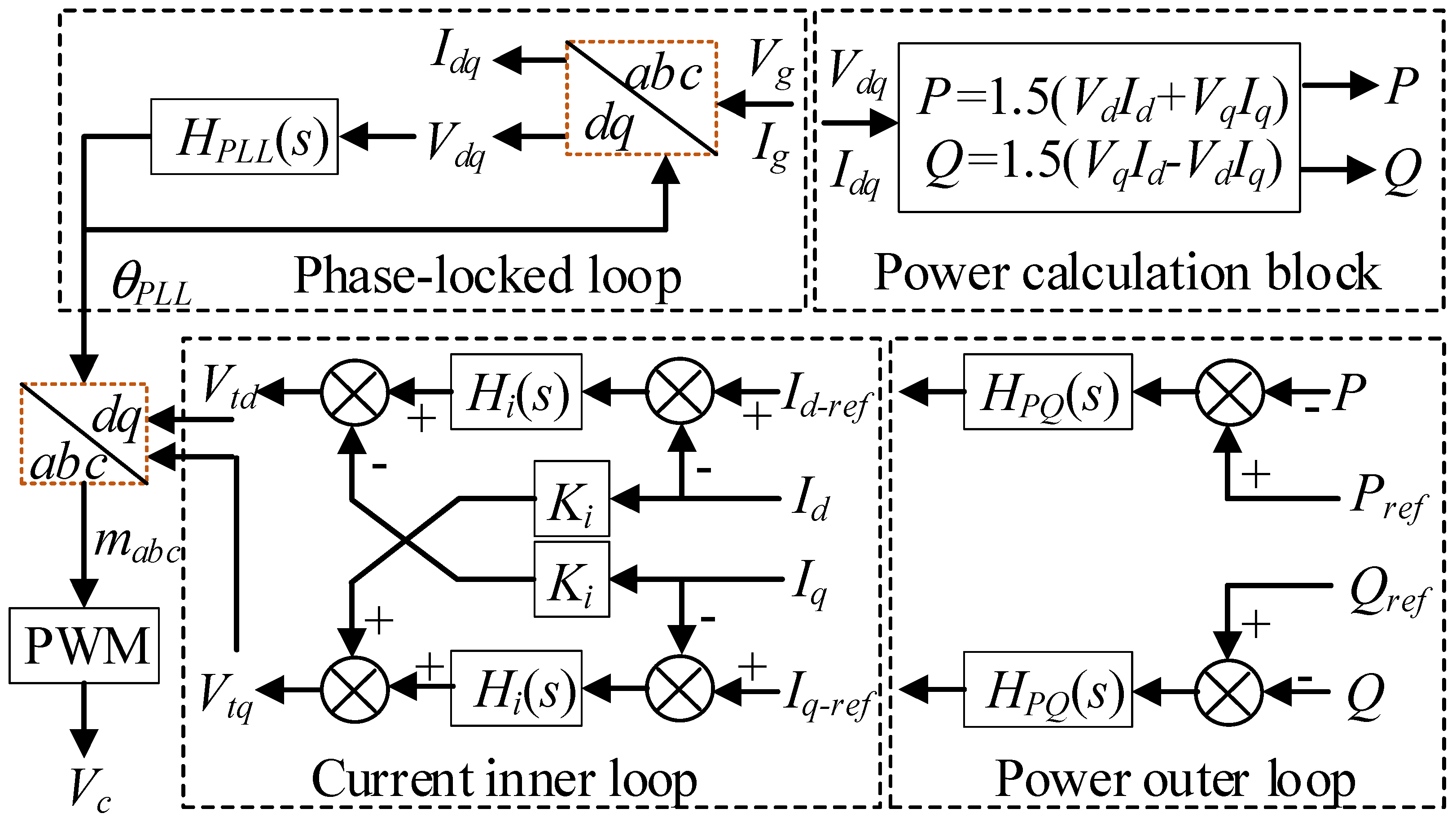
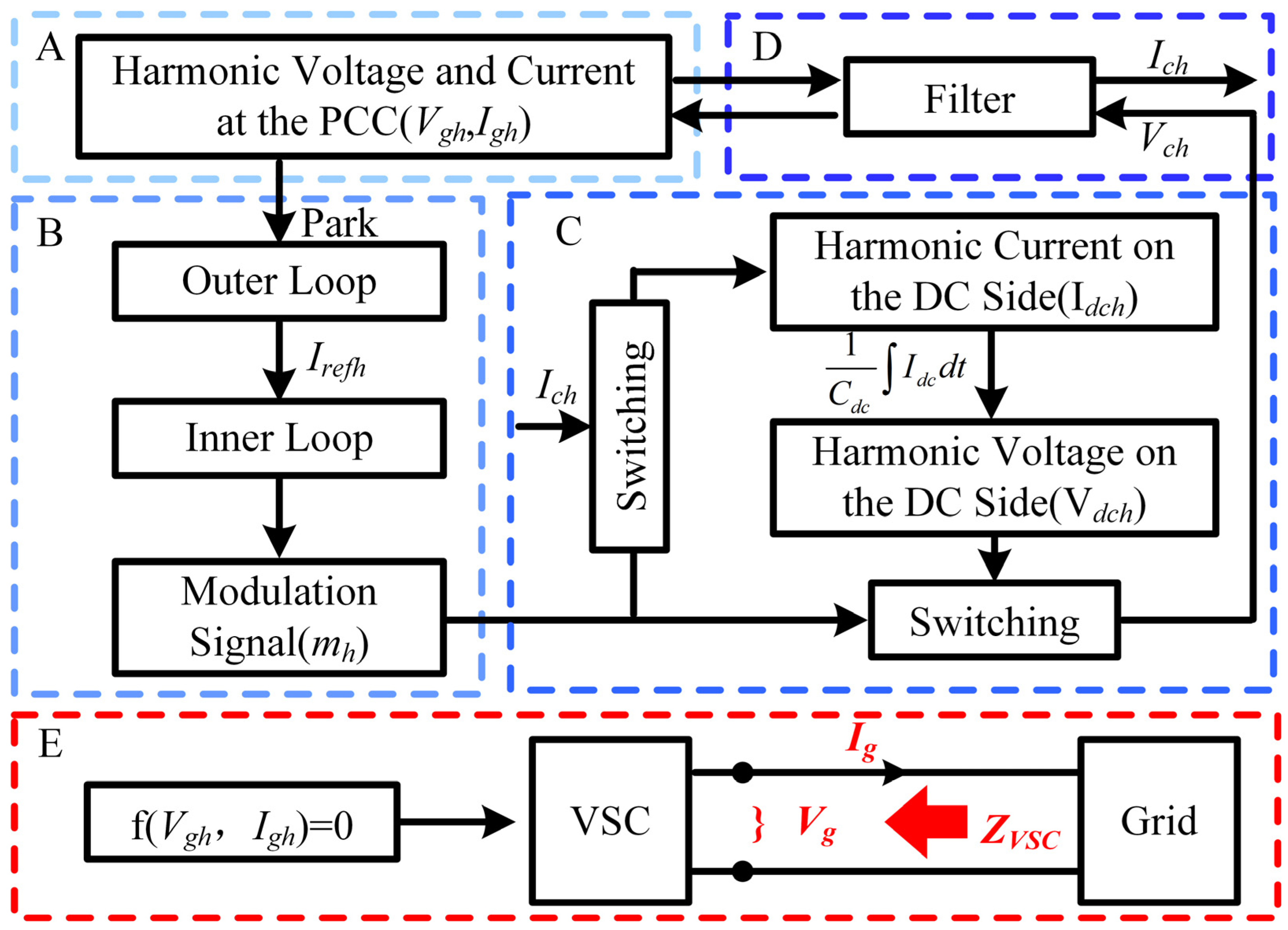
3.1. Grid-Connected PV Inverters

The impedance characteristics of grid-connected PV inverters are one of the main causes of harmonic resonance [27]. As the dynamics of the front-end DC system have a limited impact on the harmonic response of the inverter, it is reasonable to ignore the DC system and directly replace it with a capacitor [28]. Figure 4 shows the closed-loop harmonic response of a PV inverter, which clearly shows how a harmonic disturbance flows inside the inverter and induces the harmonic voltage/current at the alternating current (AC) side. Specifically, the harmonic disturbance at the AC side leads to a distorted modulation signal and the switching function via the control loop. The distorted switching function then changes the harmonic voltage at the AC side of the VSC. Meanwhile, the DC-link voltage is also affected by the harmonics at the AC side through the switching process. By mathematically calculating the harmonic response along the closed loop, we can establish the relation between the harmonic voltage and current at the Point of Common Coupling (PCC) to develop the final harmonic model of the Voltage Source Converter (VSC).

According to Figure 4, a multi-frequency harmonic voltage disturbance is assumed at the PCC. Then, the harmonic response of the control loop, the DC capacitor, and the filter are derived, which leads to the harmonic current at the PCC. The relationship between the harmonic voltage and the harmonic current of a grid-connected PV inverter can be then determined as a 2 × 2 harmonic coupling matrix, as shown in Equation (1). Please refer to [28] for detailed steps.

$$\begin{array}{l}\left[\begin{array}{c}{V}_{gm}\\ V_{gn}\end{array}\right]=\left[\begin{array}{cc}{Z}_{mm}& Z_{mn}\\ Z_{nm}& Z_{nn}\end{array}\right]\left[\begin{array}{c}{I}_{gm}\\ I_{gn}\end{array}\right]\\ (m\in h+,n\in h-,m=n+2)\end{array}$$

(1)

where Z_mm and Z_nn represent the positive sequence impedance and negative sequence impedance, respectively. Z_mn and Z_nm represent the coupling impedance. It can be demonstrated that the coupling between the positive and negative sequences follows the relationship of m = n + 2, where m is the harmonic order of the positive sequence harmonic and n is the harmonic order of the negative sequence harmonic. The detailed expressions for each impedance element are derived in Equation (2):

$$\begin{array}{l}{Z}_{mm}=\frac{-H_d(s-j{\omega }_1)H_i(s-j{\omega }_1)-H_d(s-j{\omega }_1)K_i+Z_L}{\frac{Z_L+Z_C}{Z_C}+\frac{3}{2}{H}_d(s-j{\omega }_1)H_{PQ}(s-j{\omega }_1)H_i(s-j{\omega }_1)I_{\mathrm{g}1}}\\ Z_{nn}=\frac{-H_d(s+j{\omega }_1)H_i(s+j{\omega }_1)+H_d(s+j{\omega }_1)K_i+Z_L}{\frac{Z_L+Z_C}{Z_C}+\frac{3}{2}{H}_d(s+j{\omega }_1)H_{PQ}(s+j{\omega }_1)H_i(s+j{\omega }_1)I_{\mathrm{g}1}}\\ Z_{mn}=\frac{-\frac{3}{2}{H}_d(s+j{\omega }_1)H_{PQ}(s+j{\omega }_1)H_i(s+j{\omega }_1)V_{g1}{e}^{j(2{\theta }_1)}}{\frac{Z_L+Z_C}{Z_C}+\frac{3}{2}{H}_d(s-j{\omega }_1)H_{PQ}(s-j{\omega }_1)H_i(s-j{\omega }_1)I_{\mathrm{g}1}}\\ Z_{nm}=\frac{-\frac{3}{2}{H}_d(s-j{\omega }_1)H_{PQ}(s-j{\omega }_1)H_i(s-j{\omega }_1)V_{g1}{e}^{j(-2{\theta }_1)}}{\frac{Z_L+Z_C}{Z_C}+\frac{3}{2}{H}_d(s+j{\omega }_1)H_{PQ}(s+j{\omega }_1)H_i(s+j{\omega }_1)I_{\mathrm{g}1}}\end{array}$$

(2)

In Equation (2), H_d(s) = e^−1.5τs represents the transfer function of the sampling delay component, where $\tau$ is the sampling period. Moreover, Z_L and Z_C denote the harmonic impedances of the inverter-side filtering inductor and filtering capacitor, respectively. The definitions of other variables can be found in Figure 2.

It should be mentioned that the frequency coupling strength of PV inverters is relatively small [28], since the coupling impedance (Z_mn/Z_nm) is much smaller than the self-impedance (Z_mm/Z_nn). As a result, the harmonic coupling matrix can be further decoupled into positive and negative sequence impedances, i.e., Z_mm/Z_nn.

3.2. Collector Lines

Regarding collector lines, the lumped $\pi$ model is commonly used for harmonic studies, as shown in Figure 5, where the parameters are defined by Equation (3).

$$\left\{\begin{array}{l}{Z}_{Line-R} =l{R}_0\\ Z_{Line-L} =lj\omega L_0\\ Z_{Line-C} =l/j\omega C_0\end{array}\right.$$

(3)

In Equation (3), l represents the actual length of the collector line. R₀, L₀, and C₀ represent the resistance, inductance, and capacitance per unit length of the collector line, respectively. The feasible frequency range to use the lumped $\pi$ model can be determined by Equation (4).

$$l_c=\frac{150}{h}(\mathrm{km})$$

(4)

where the parameter l_c represents the critical length of the collector line and h denotes the harmonic order. When the actual length l of the collector line is shorter than the critical length l_c, the lumped parameter model can be used with confidence. Otherwise, the distributed $\pi$ model must be used. Since the length of the collector lines between adjacent PV generators is generally below 5 km, the lumped $\pi$ model is applicable as long as the harmonic order of interest is below 30 harmonics.

3.3. Double-Split Transformer

The impedance model of a double-split transformer is shown in Figure 6, where number 1 and 2 represent the two low-voltage windings, and number 3 represents the high-voltage winding of the double split transformer; Z₁ and Z₂ represent the equivalent impedances of the two low-voltage windings, and Z₃ represents the equivalent impedance of the high-voltage winding. The values of Z₁, Z₂, and Z₃ can be determined by Equation (5).

$$\left\{\begin{array}{l}{Z}_1=Z_2=\frac{K_f}{2}{Z}_p\\ Z_3=(1-\frac{K_f}{4})Z_p\end{array}\right.$$

(5)

$$K_f=\frac{Z_f}{Z_p}$$

(6)

In Equations (5) and (6), Z_p is the short-circuit impedance at which the two low-voltage windings operate in parallel, while Z_f is the short-circuit impedance at which the two low-voltage windings operate independently. K_f is the split factor, which typically ranges from 0 to 4 and depends on the relative positions of the two low-voltage windings in the double-split transformer.

3.4. Complete Impedance Model

Once the impedance models of the PV inverter, the transformer, and the collector line are established, the complete impedance model of the PV plant can be established based on the network topology. The overall impedance model for the PV power plant at the site level is depicted in Figure 7, where the two dashed boxes represent the detailed structures of the collector line and PV unit respectively.

Using the network transformation method, the impedance network shown in Figure 7 is equivalently transformed into the aggregated impedance model shown in Figure 8, where the blue dashed line means the equivalence is done for the PV system, whereas the AC system remains the same.

Here, Z_PV-GET is calculated by the equivalent impedance of the two feeders, i.e., $Z_5^1$ and $Z_5^2$, by Equation (7).

$$Z_{PV-GET}=Z_5^1//Z_5^2$$

(7)

The superscripts of $Z_5^1$ and $Z_5^2$ represent the first and second feeders, respectively, while the subscripts of $Z_5^1$ and $Z_5^2$ represent the number of PV units in the first and second feeders, respectively. The values of $Z_5^1$ and $Z_5^2$ can be obtained based on Equation (8).

$$\begin{array}{l}{Z}_1^k=(1/Y_l)//Z_{PV}//(Z_{PV}//Y_l+Z_l)\\ ......\\ Z_{n-1}^k=Y_l//Z_{PV}//(Z_{n-2}^k//Y_l+Z_l)\\ Z_n^k=Y_l//(Z_{n-1}^k//Y_l+Z_l)\end{array}$$

(8)

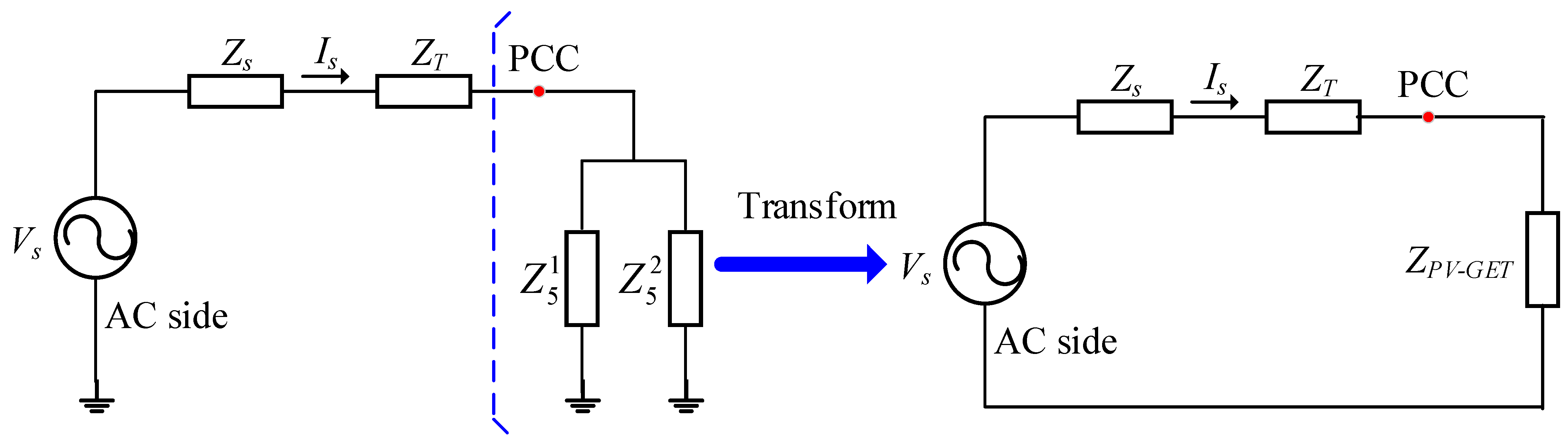
4. Dynamic Equivalent Model of the PV Plant

Although the model developed in Section 3 is accurate, it is not widely used in the industry because the analytical modeling process is theoretically complicated and time-consuming. Alternatively, the utility prefers to utilize electromagnetic transient simulation models with frequency scan techniques. Due to software limitations, it is very challenging to run detailed PV plant models in commercial simulation platforms, such as MATLAB/Simulink and PSCAD/EMTDC. A common solution is to replace the detailed model with the dynamic equivalent model of the plant, as shown in Figure 9.

According to Figure 9, multiple serially or parallelly connected PV units in Figure 1 are replaced by a single equivalent PV unit in Figure 8. Similarly, multiple double-split transformers are replaced by a single double-winding transformer, and the complex topology of the collector lines is simplified to a single segment. The step-up transformer and the AC system remain unchanged. Such a practice significantly reduces the modeling complexity and improves the efficiency of the frequency scan.

The following two requirements are commonly considered in the development of the equivalent model: First, the total rated capacity should remain unchanged before and after the equivalence process. This means that the active and reactive power outputs of the equivalent model should match those of the detailed model at the PCC, as shown in Equation (9). Second, the voltage at the PCC should remain unchanged before and after the equivalence process, as shown in Equation (10).

$$\left\{\begin{array}{l}{P}_{PVeq}={\displaystyle \sum _{i=1}^n{P}_{PVi}}\\ Q_{PVeq}={\displaystyle \sum _{i=1}^n{Q}_{PVi}}\end{array}\right.$$

(9)

$$V_{pcceq}=V_{pcci}$$

(10)

where subscript “eq” represents the equivalent system; subscript “i” represents the i-th PV generation unit, and “n” represents the total number of PV generation units in the power plant.

Next, the parameters of the PV generation units (including the control and filter parameters of the PV inverter), transformers, and collector lines in the equivalent model will be determined.

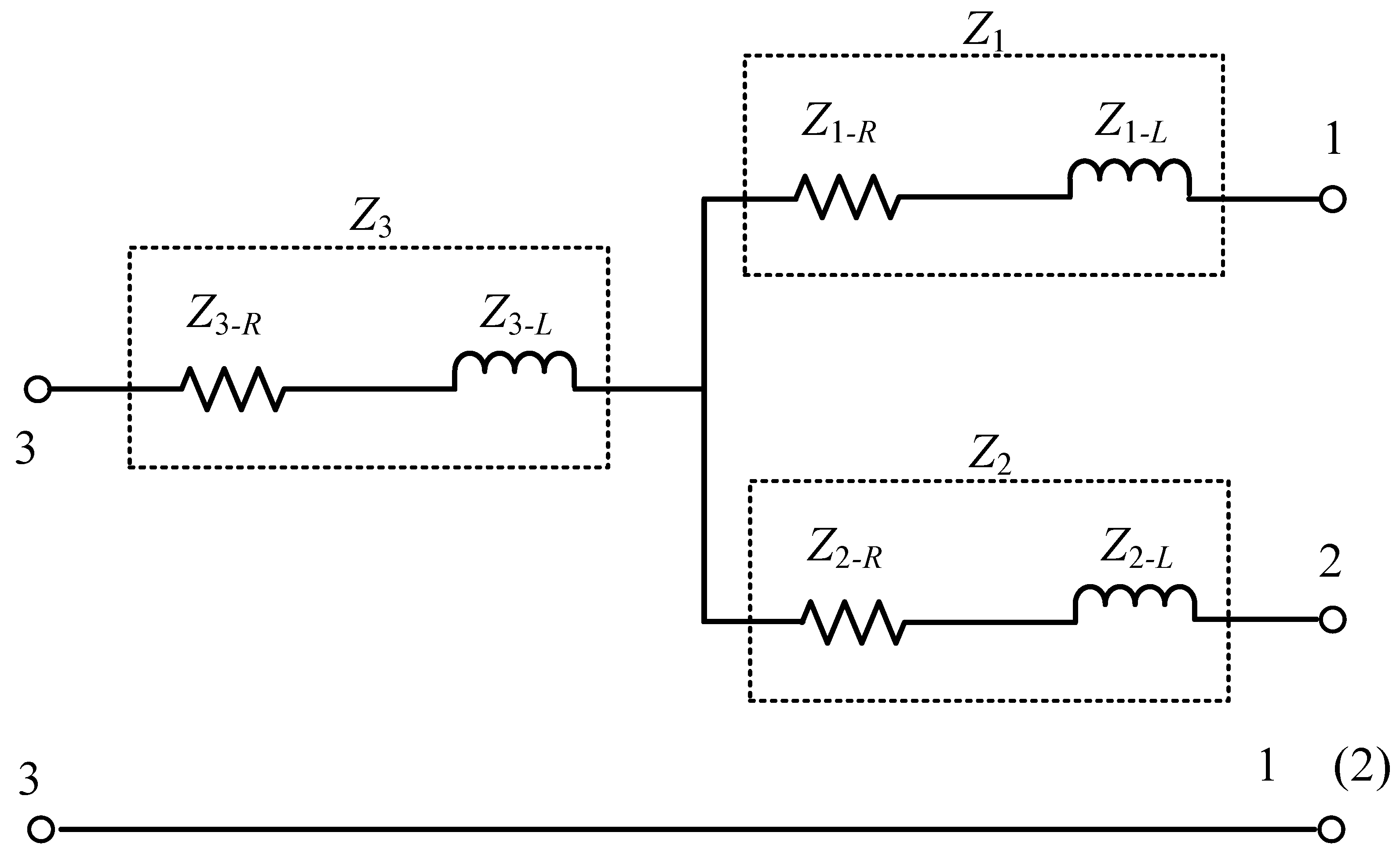
4.1. Equivalent Parameters of the PV Inverters

Due to the identical configuration and parameters of each PV array unit in the plant and the adoption of a power control strategy, the equivalent model of the inverter involves aggregating 20 inverters with a capacity of 500 kW each into a single inverter with a capacity of 10 MW. Since the simulation model utilizes per unit values for control, the control parameters remain unchanged. Considering the filtering effect of the grid-tied inverters and the need to ensure that the reactive power consumption of the aggregated inverter model matches the sum of the reactive power consumption of the individual inverters before aggregation, the aggregation formulas for the DC-side capacitance C_dc, filtering inductance L, and filtering capacitance C are given as Equation (11).

$$\left\{\begin{array}{cc}{C}_{dceq}=n{C}_{dci}& C_{eq}=n{C}_i\\ \frac{1}{L_{1eq}}=n\frac{1}{L_{1i}}& \frac{1}{L_{2eq}}=n\frac{1}{L_{2i}}\end{array}\right.$$

(11)

4.2. Equivalent Parameters of the Transformers

The impedance of the step-up transformer can be considered part of the network-side inductance of the LCL filter. According to Equation (11), the reciprocal of the inductance of the distribution transformer in the equivalent model is the sum of the reciprocals of the distribution transformer inductances in each PV unit of the power plant. It is important to note that the impedance voltage on the transformer nameplate is expressed in per-unit values. Therefore, the parameters of the transformer in the equivalent system can be directly determined based on the aggregated power. This means that only the capacity of the transformer is increased to the sum of the capacities of the parallel transformers without changing the per-unit values of the short-circuit impedance.

4.3. Equivalent Parameters of the Collector Lines

In this paper, the power loss conservation method is adopted to calculate the equivalent parameters of the collector lines. The core idea is to maintain the power loss of the collector lines unchanged before and after equivalence. As Figure 1 shows, the plant consists of both radial and parallel collector lines. Therefore, it is necessary to calculate the equivalent parameters for each type.

In the case that multiple PV inverters are connected in series along a feeder, the equivalence calculation formula is as follows:

$$\begin{array}{l}{S}_{de}=S_{Z1}+S_{Z2}+\cdots \cdots +S_{Zn}\\ ={(I_1+I_2+\cdots \cdots +I_n)}^2{Z}_1\\ +{(I_1+I_2+\cdots \cdots +I_{n-1})}^2{Z}_2\cdots \cdots +I_n{}^2{Z}_n\\ S_{eq}={(I_1+I_2+\cdots \cdots +I_n)}^2{Z}_{eq}\\ S_{de}=S_{eq}\end{array}$$

(12)

where S_de is the total apparent power of a feeder, S_eq is the total apparent power of the feeder after equivalence, n represents the number of segments of the collector lines in a feed line, and I represents the current injected into the feeder by each PV unit through the distribution transformer. In many cases, I₁ = I₂ … = I_n = I, and Z₁ = Z₂ = … Z_n = Z; then, we have:

$$Z_{eq}=\frac{n(1+n)(2n+1)Z}{6n^2}$$

(13)

In the case that no PV inverters are connected in series and all PV inverters are connected in parallel, the equivalence calculation formula is as follows:

$$\begin{array}{l} S_{de}=S_{Z1}+S_{Z2}+\cdots \cdots +S_{Zn}\\ =I_1{}^2{Z}_1+I_2{}^2{Z}_2+\cdots \cdots +I_n{}^2{Z}_n\\ S_{eq}={(I_1+I_2+\cdots \cdots +I_n)}^2{Z}_{eq}\\ S_{de}=S_{eq}\end{array}$$

(14)

If I₁ = I₂ = … I_n = I and Z₁ = Z₂ = … Z_n = Z, then we have:

$$Z_{eq}=\frac{Z}{n}$$

(15)

Equations (12) and (14) represent the equivalent calculation formulas for the resistance and inductance of the collector lines. Regarding the capacitance of the collector line, if we neglect the voltage differences between PV units, the equivalent capacitance can then be calculated as the summation of the capacitance of the collector lines on the same feeder.

5. Comparative Study

In this section, a comparative study on the accurate impedance model and the equivalent impedance model is conducted using the PV system described in Section 2. A harmonic resonance study of the PV system is also presented. The key parameters of the system are listed in

Table 2. Main parameters of the PV inverters.

Parameter	Value	Parameter	Value
Rated line voltage	690	Direct current Capacitor/μF	1300
Filter inductance/mH	1	Filter capacitance/μF	100
Outer loop power control PI KiPQ	4	Outer loop power control PI KpPQ	0.04
Current inner loop PI Kii	200	Current inner loop PI Kpi	0.6

,

Table 3. Main parameters of the collector lines.

Cross-Section of the Cable/(mm2)	Resistance/(Ω/km)	Inductance/(mH/km)	Capacitance/(μF/km)
50	0.3448	2.51681	0.163398
95	0.1815	2.45092	0.205812
120	0.1437	2.42775	0.224132
185	0.0932	2.38438	0.264385
240	0.0718	2.35517	0.296633
300	0.0575	2.33258	0.324904

and

Table 4. Main parameters of the double-split transformer.

Parameter	Value
Transformer ratio/kV	35/0.69
Short-circuit impedance/%	8
Fission coefficient	3.5
Rated capacity/kVA	1250
Connected group	D,yn11-yn11

.

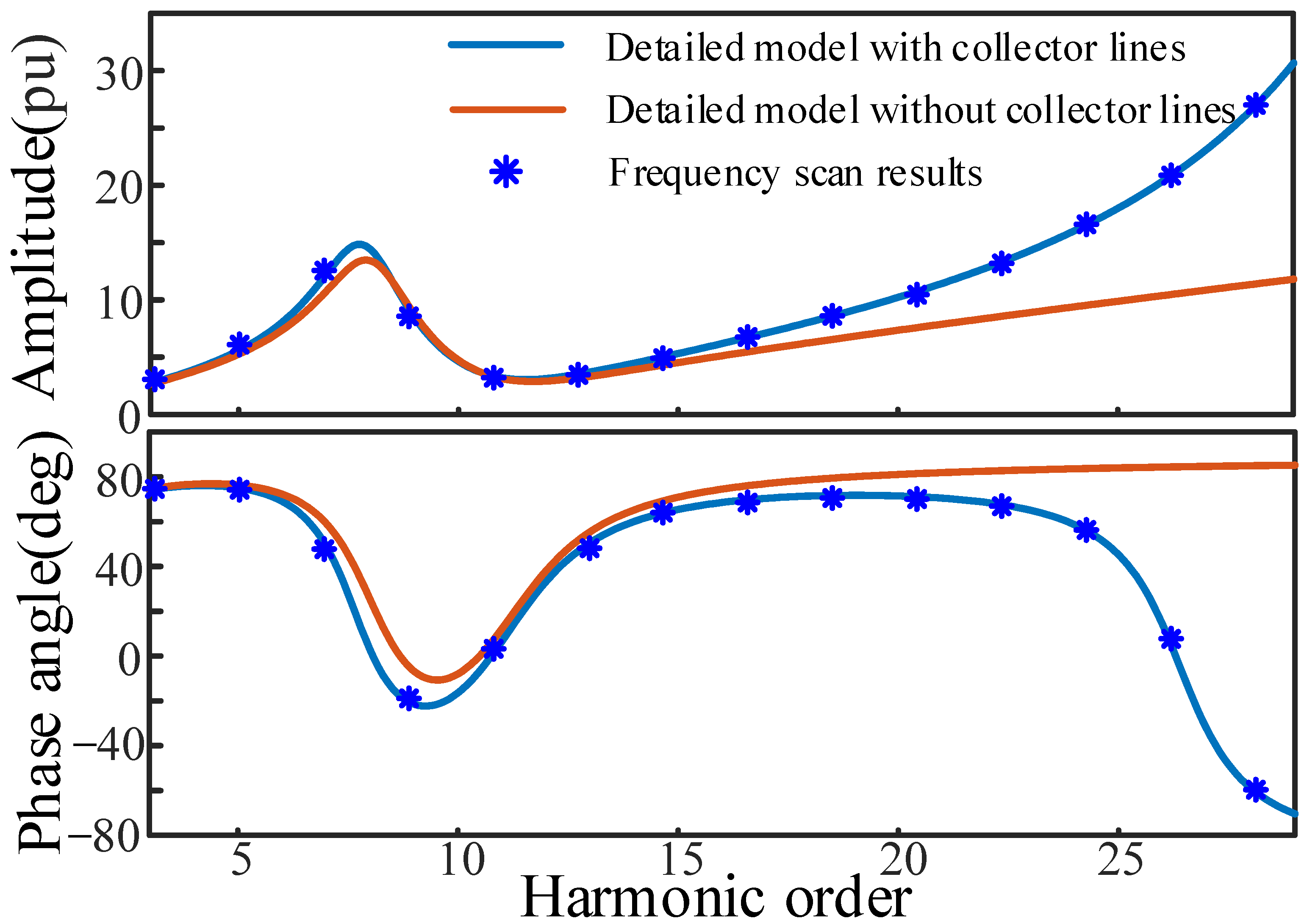
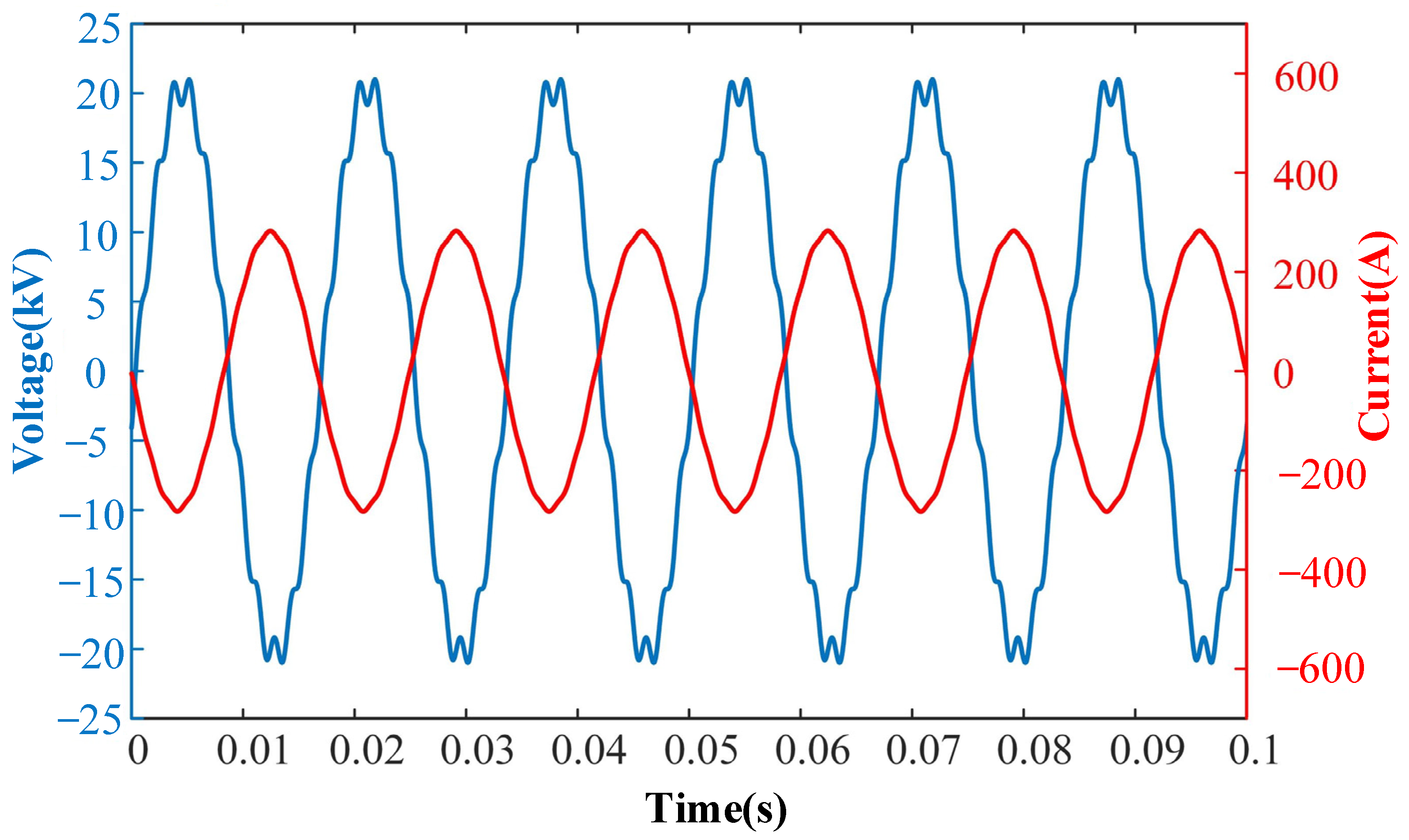
5.1. Validation of Detailed Model

The detailed model of the PV plant is established using the bottom-up method, and the results are shown in Figure 10. In the figure, frequency scan results marked by blue stars indicate the impedance determined by the frequency scan of a detailed PV plant in MATLAB/Simulink; thus, it can be regarded as a benchmark in comparison. The blue line indicates the calculated detailed model of the PV system with collector lines. The consistency between the blue line and the blue stars demonstrates the high accuracy of the detailed model.

In many studies, the influence of the collector lines is overlooked when establishing the impedance model of a PV plant. To verify the feasibility of this assumption, the impedance of the detailed model that neglects the collector lines is also depicted in Figure 10, which is marked in red. The results indicate that such a practice can introduce significant errors in the impedance model of the PV plant, especially in the high frequency range. The reason is that the shunt capacitor of the collector line has a more significant impact at high frequency ranges; thus, it cannot be ignored.

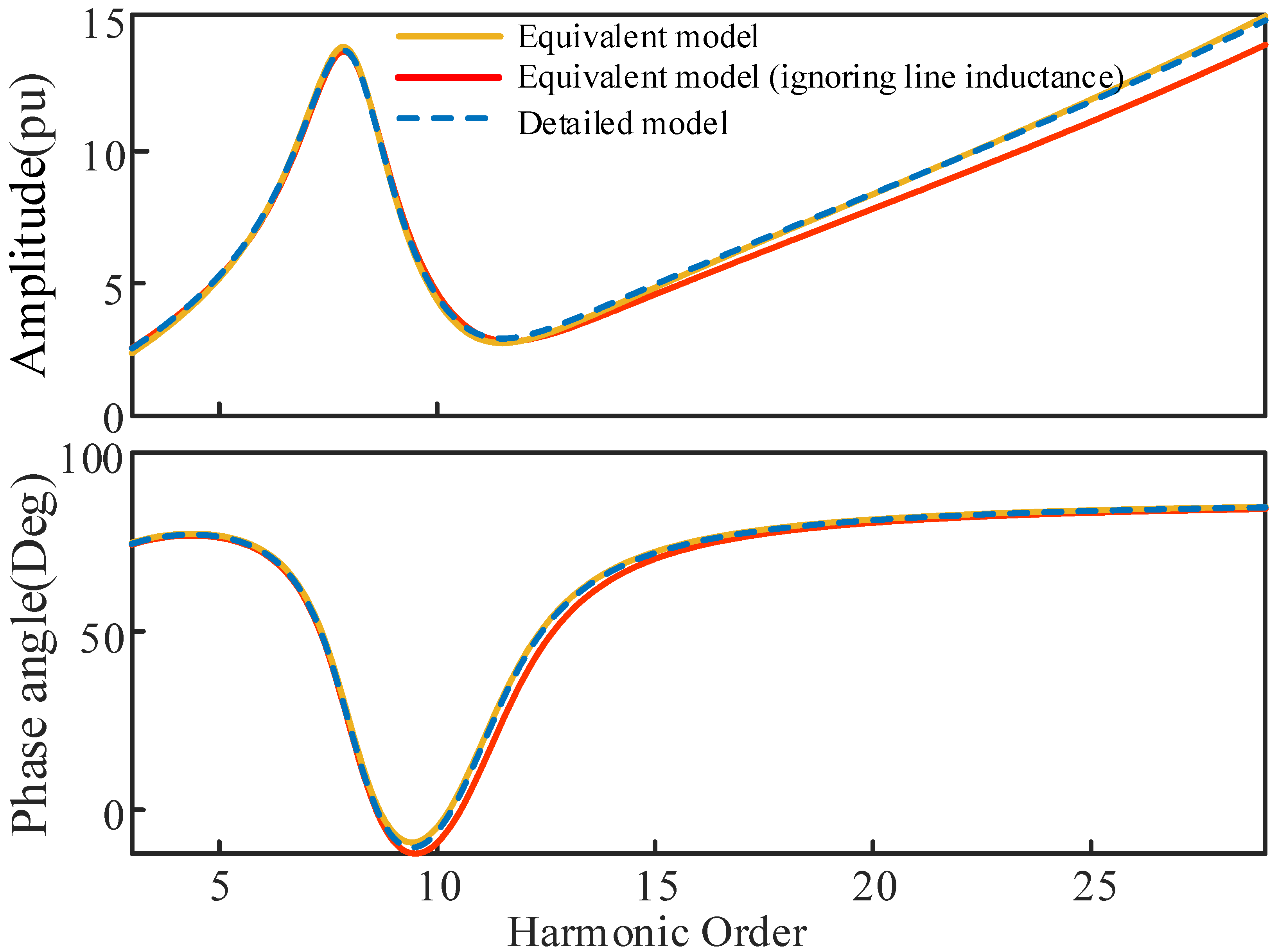
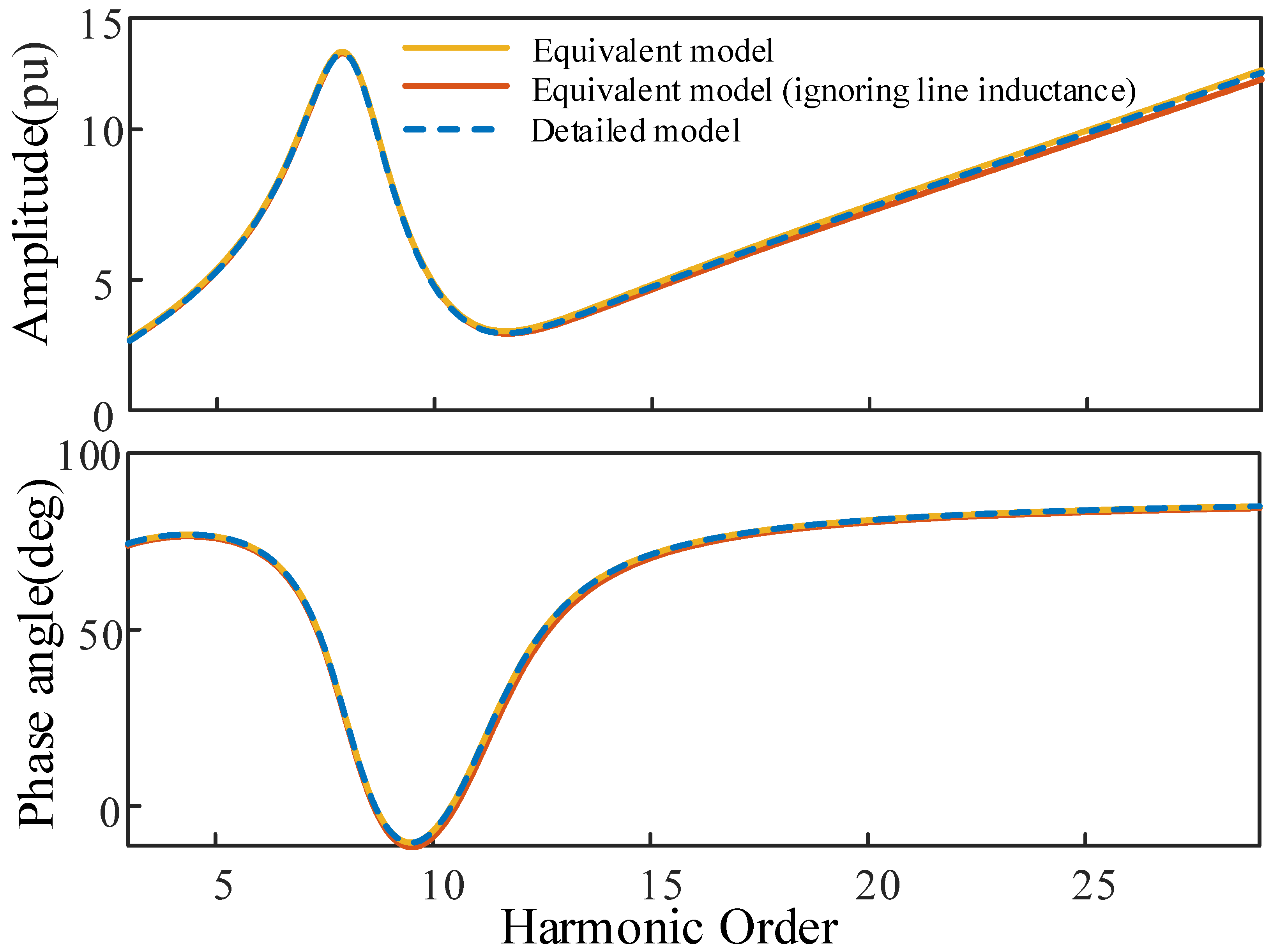
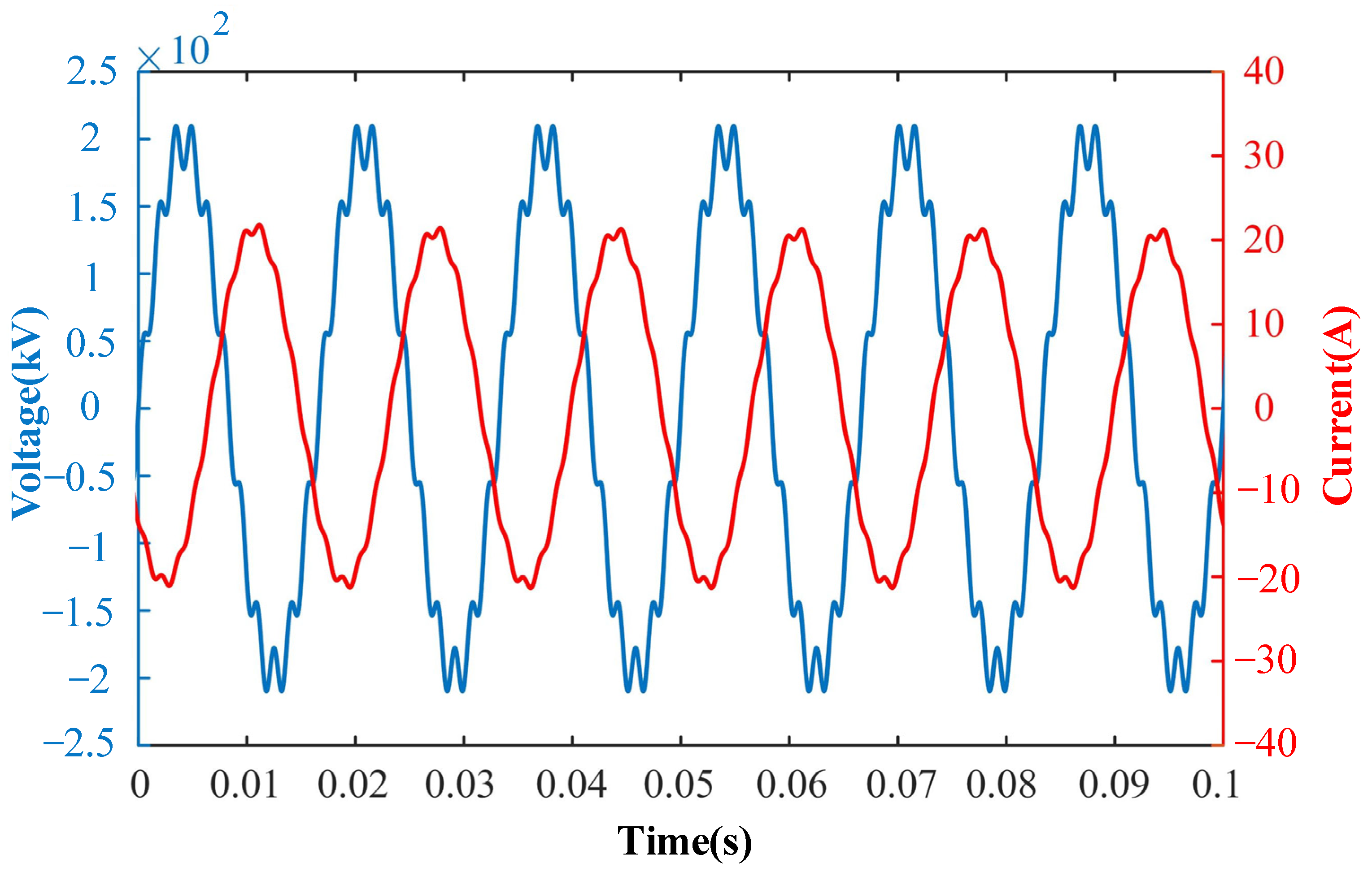
5.2. Validation of the Dynamic Equivalent Model

From Table 3, it can be observed that the unit resistance and inductance of the collector lines increase as the cross-sectional area decreases, while the unit capacitance decreases with the cross-sectional area. The longer the cable length is, the larger the inductance at the same frequency, which means a greater impact on the impedance aggregation of the PV plant. However, the series impedance of the collector lines is generally much smaller than the impedance of the PV generation units. Therefore, it is possible to replace the π-circuit model of a collector line as a capacitor.

When a ZC-YJV22 3 × 50 mm² underground cable with a length of 5 km is used in the PV plant, a comparison is conducted between the detailed model and the dynamic equivalent model of the PV plant, as shown in Figure 11. According to the figure, it can be observed that the frequency response of the dynamic equivalent model obtained by the power loss conservation method is highly consistent with the detailed model across the entire frequency range. On the other hand, the equivalent model that ignores the line inductance also matches well with the detailed model within the harmonic range up to the 13th harmonic, but the discrepancy increases to 10% at the 30th harmonic.

The above analysis demonstrates that the dynamic equivalent model can be used for harmonic resonance analysis with confidence. The key is to model the equivalent capacitance of the collector line, whereas the impact of the series impedance of the collector line is much smaller. Regarding practical PV plants [8], the cross-sectional area of the collector lines ranges from 3 × 95 to 3 × 185 mm², and the length of the collector lines ranges from 0.5 to 2.5 km. Therefore, another comparison is made considering a ZC-YJV22 3 × 120 mm² underground cable with a length of 1.5 km, which represents the average parameters in practical PV plants. The results are shown in Figure 12.

According to Figure 12, it can be observed that the impedance of the equivalent model obtained by neglecting the series impedance closely matches the impedance of the detailed model across the entire frequency range. The maximum impedance error is only 3.25%. The result indicates that for most PV plants, Equations (12)–(15) are not needed to calculate the equivalent series impedance of the collector line. Such a finding significantly simplifies the modeling process of the PV plant and enhances the confidence of frequency scan results.

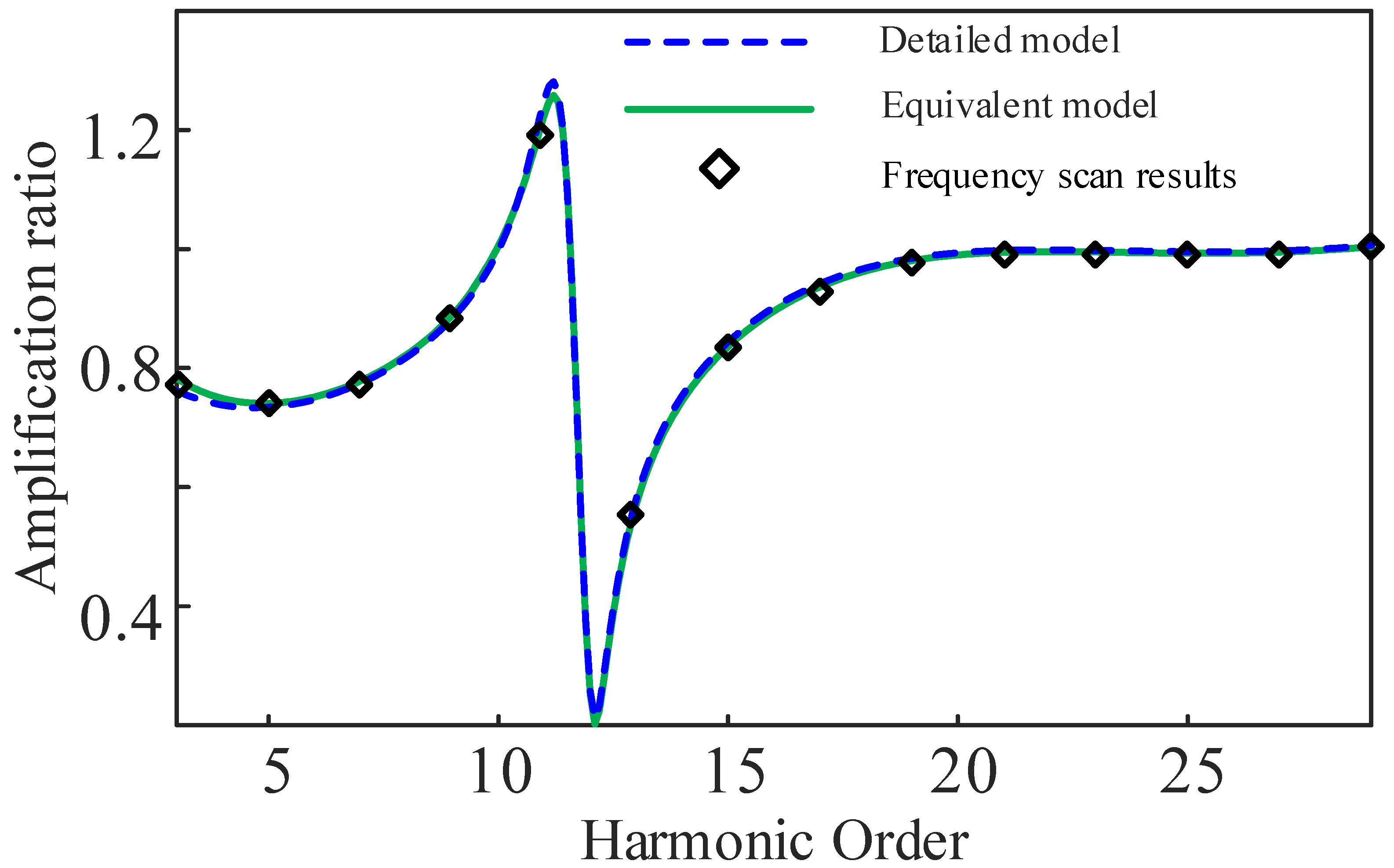
5.3. Harmonic Resonance Analysis

Based on the impedance model developed above, a harmonic resonance study that involves a 10 MW PV plant and a ±3 Mvar Static Synchronous Compensator (STATCOM) is presented in this section, as shown in Figure 13. The control structure and parameters of the STATCOM are consistent with those specified in [28], as shown in

Table 5. Main parameters of the STATCOM.

Parameter	Value	Parameter	Value
Rated line voltage	2165 V	DC voltage	5000 V
Filter inductance	0.8 mH	Filter capacitance	45 µF
AC voltage PI Kiac	2500	AC voltage PI Kpac	0.55
DC voltage PI Kidc	0.15	DC voltage PI Kpdc	0.001
current PI Kii	200	current PI Kpi	0.8

.

To validate the feasibility of the equivalent impedance model for harmonic resonance analysis, harmonics ranging from the 3rd to the 29th are added to the voltage at the grid side. Figure 14 and Figure 15 show the time-domain simulation results of the voltage and current of the PCC and the 220 kV bus, respectively, when the 11th and 13th harmonics are considered.

The harmonic amplification ratio at the PCC point (35 kV side) is calculated using the ratio of the harmonic voltage with and without the connection of the PV plant. This measured ratio is then compared with the analytical value calculated using the detailed impedance model and the equivalent impedance model. The results, as shown in Figure 16, demonstrate the effectiveness of the equivalent model for the harmonic resonance study. As seen from the figure, the connection of the PV plant amplifies approximately the 11th harmonic for a ratio of 1.2.

Figure 17 shows the harmonic amplification ratios under different operating conditions of the PV system. These ratios are calculated using the detailed impedance models of the PV system under different power outputs. It can be seen that the amplification ratios remain almost constant regardless of the output power of the PV units. The reason is that the Phase Locked Loop (PLL), the power outer loop, and the DC capacitor of the PV unit have limited impact on the frequency response at the harmonic frequency. As a result, the harmonic model of the entire PV system is approximately linear, which will not be affected by the operating condition of the system. This finding indicates that the harmonic resonance study in one operating condition is sufficient.

6. Conclusions

In this paper, the feasibility of the dynamic equivalent model in a harmonic resonance study is investigated using a real-life PV plant. For this purpose, a detailed harmonic model of the PV plant is established using the bottom-up modeling technique, which is regarded as the benchmark for comparison, while the dynamic equivalent model is established based on the principle of power loss conservation. The following conclusions are drawn:

• The equivalent model exhibits good consistency with the detailed model across the entire frequency range. Therefore, the frequency scan result of the dynamic equivalent model can be used for harmonic resonance analysis with confidence.
• The collector lines between the PV units have a significant impact on the impedance models of the plant at the harmonic frequency. Therefore, the assumption of ignoring collector lines that has been used in many papers is not acceptable.
• The capacitance of the collector line has a dominant impact on the harmonic impedance of the PV plant, while the impact of the series impedance is much smaller. If a precise quantitative analysis is not needed, the equivalent model of the collector line can be further simplified as a capacitor. The error is expected to be below 10%, if the harmonic order of interest is not higher than the 30th harmonic.

References

1. Liu, F.; Mu, Y.; Chen, Z. Control Strategy for Improving the Voltage Regulation Ability of Low-Carbon Energy Systems with High Proportion of Renewable Energy Integration. Electronics 2023, 12, 2513. [Google Scholar] [CrossRef]
2. Tong, D.; Farnham, D.J.; Duan, L.; Zhang, Q.; Lewis, N.S.; Caldeira, K.; Davis, S.J. Geophysical constraints on the reliability of solar and wind power worldwide. Nat. Commun. 2021, 12, 6146. [Google Scholar] [CrossRef]
3. Gao, B.; Wang, Y.; Xu, W. Modeling Voltage Source Converters for Harmonic Power Flow Studies. IEEE Trans. Power Deliv. 2021, 36, 3426–3437. [Google Scholar] [CrossRef]
4. Dai, L.; Wang, H.; Qin, Y.; Shi, G.; Zhang, J.; Cai, X. Analysis and Suppression of High-Frequency Resonance for Offshore Wind Power Grid-Connected Converter Considering Cable Capacitance Effect. Electronics 2023, 12, 2638. [Google Scholar] [CrossRef]
5. Gao, B.; Wang, Y.; Xu, W. An Improved Model of Voltage Source Converters for Power System Harmonic Studies. IEEE Trans. Power Deliv. 2022, 37, 3051–3061. [Google Scholar] [CrossRef]
6. Zheng, T.; Kong, F.; Li, G.; Wang, Z.; Chen, Y. A Gray-Box Stability Analysis Method of Grid-Connected Inverter Considering Synchronization Dynamics. Electronics 2023, 12, 2509. [Google Scholar] [CrossRef]
7. Ackermann, T. Transmission systems for offshore wind farms. IEEE Power Eng. Rev. 2003, 22, 23–27. [Google Scholar] [CrossRef]
8. Liu, Q.; Liu, F.; Zou, R.; Li, Y. Harmonic Resonance Characteristic of Large-scale PV Plant: Modelling, Analysis and Engineering Case. IEEE Trans. Power Deliv. 2022, 37, 2359–2368. [Google Scholar] [CrossRef]
9. Zhang, D.; Chen, X.; Yang, S. Analysis of High-Frequency Resonance and Suppression Strategy of Photovoltaic Power Plant with Static Reactive Power Compensation Device. Proc. CSEE 2022, 1–15. [Google Scholar]
10. Buchhagen, C.; Rauscher, C.; Menze, A.; Jung, J. BorWin1—First Experiences with harmonic interactions in converter dominated grids. In Proceedings of the International ETG Congress 2015; Die Energiewende—Blueprints for the Renewable Energy Age, Bonn, Germany, 17–18 November 2015; pp. 1–7. [Google Scholar]
11. Ning, X.; An, L.; Ma, F. Harmonic interaction between large-scale photovoltaic power stations and grid. Proc. CSEE 2013, 33, 9–16. [Google Scholar]
12. Qin, S.; Li, S.; Wang, R. Resonance and suppression strategy of large-capacity permanent magnet synchronous generator wind turbine system. Autom. Electr. Power Syst. 2014, 38, 11–16. [Google Scholar]
13. Wang, L.; Xie, X.; Jiang, Q.; Liu, H.; Li, Y.; Liu, H. Investigation of SSR in Practical DFIG-Based Wind Farms Connected to a Series-Compensated Power System. IEEE Trans. Power Syst. 2015, 30, 2772–2779. [Google Scholar] [CrossRef]
14. Erlich, I.; Feltes, C.; Shewarega, F. Enhanced Voltage Drop Control by VSC–HVDC Systems for Improving Wind Farm Fault Ridethrough Capability. IEEE Trans. Power Deliv. 2014, 29, 378–385. [Google Scholar] [CrossRef]
15. Ren, Y.; Wang, X.; Chen, L.; Min, Y.; Li, G.; Wang, L.; Zhang, Y. A Strictly Sufficient Stability Criterion for Grid-Connected Converters Based on Impedance Models and Gershgorin’s Theorem. IEEE Trans. Power Deliv. 2020, 35, 1606–1609. [Google Scholar] [CrossRef]
16. Messo, T.; Luhtala, R.; Aapro, A.; Roinila, T. Accurate Impedance Model of Grid-Connected Inverter for Small-Signal Stability Assessment in High-Impedance Grids. In Proceedings of the 2018 International Power Electronics Conference, Niigata, Japan, 20–24 May 2018; pp. 3156–3163. [Google Scholar] [CrossRef]
17. Ren, W.; Larsen, E. A Refined Frequency Scan Approach to Sub-Synchronous Control Interaction (SSCI) Study of Wind Farms. IEEE Trans. Power Syst. 2016, 31, 3904–3912. [Google Scholar] [CrossRef]
18. Wang, Y. Vector-fitting-based quantitative ssci analysis for Seriescompensated wind power systems. IET Renew. Power Gener. 2020, 14, 3023–3034. [Google Scholar] [CrossRef]
19. Zhu, L.; Hu, X.; Li, S. High-Frequency Resonance of DFIG-Based Wind Generation under Weak Power Network. In Proceedings of the 2018 International Conference on Power System Technology, Guangzhou, China, 10–12 September 2018; pp. 2719–2724. [Google Scholar] [CrossRef]
20. Wang, Y.; Jiang, X.; Xie, X.; Yang, X.; Xiao, X. Identifying Sources of Subsynchronous Resonance Using Wide-Area Phasor Measurements. IEEE Trans. Power Deliv. 2021, 36, 3242–3254. [Google Scholar] [CrossRef]
21. Liu, H.; Xie, X.; He, J.; Xu, T.; Yu, Z.; Wang, C.; Zhang, C. Subsynchronous Interaction Between Direct-Drive PMSG Based Wind Farms and Weak AC Networks. IEEE Trans. Power Syst. 2017, 32, 4708–4720. [Google Scholar] [CrossRef]
22. Liu, H.; Xie, X.; Zhang, C.; Li, Y.; Liu, H.; Hu, Y. Quantitative SSR Analysis of Series-Compensated DFIG-Based Wind Farms Using Aggregated RLC Circuit Model. IEEE Trans. Power Syst. 2017, 32, 474–483. [Google Scholar] [CrossRef]
23. Remon, D.; Cantarellas, A.M.; Rodriguez, P. Equivalent Model of Large-Scale Synchronous Photovoltaic Power Plants. IEEE Trans. Ind. Appl. 2016, 52, 5029–5040. [Google Scholar] [CrossRef]
24. Li, W.; Chao, P.; Liang, X.; Ma, J.; Xu, D.; Jin, X. A Practical Equivalent Method for DFIG Wind Farms. IEEE Trans. Sustain. Energy 2018, 9, 610–620. [Google Scholar] [CrossRef]
25. Hussein, D.N.; Matar, M.; Iravani, R. A Type-4 Wind Power Plant Equivalent Model for the Analysis of Electromagnetic Transients in Power Systems. IEEE Trans. Power Syst. 2013, 28, 3096–3104. [Google Scholar] [CrossRef]
26. Shao, H.; Yan, H.; Cai, X.; Qin, Y.; Zhang, Z. Aggregation Modeling Algorithm of PMSM Wind Farm Considering Submarine Cable Power Loss. In Proceedings of the 2021 IEEE 12th Energy Conversion Congress & Exposition—Asia (ECCE-Asia), Singapore, 24–27 May 2021; pp. 1169–1174. [Google Scholar] [CrossRef]
27. Wang, S.; Li, Y.; Zhang, M.; Peng, Y.; Tian, Y.; Lin, G.; Chang, F. Harmonic Resonance Suppression with Inductive Power Filtering Method: Case Study of Large- Scale Photovoltaic Plant in China. IEEE Trans. Power Electron. 2023, 38, 6444–6454. [Google Scholar] [CrossRef]
28. Wang, Y.; Chen, H.; Gao, B.; Xiao, X.; Torquato, R.; Trindade, F.C. Harmonic resonance analysis in high-renewable-energy-penetrated power systems considering frequency coupling. Energy Convers. Econ. 2022, 3, 333–344. [Google Scholar] [CrossRef]
Figure 1. Topological structure of a PV plant.
Electronics 12 03746 g001
Figure 2. Dual-loop control of the PV inverter.
Electronics 12 03746 g002
Figure 3. Impedance Modeling Process of a Large PV Plant.
Electronics 12 03746 g003
Figure 4. Explanation of the harmonic response of the PV inverter. (A) Harmonic measurement; (B) Control loop; (C) AC/DC interaction; (D) Filter; (E) Grid connection.
Electronics 12 03746 g004
Figure 5. Impedance Model of the Collector Lines.
Electronics 12 03746 g005
Figure 6. Impedance model of a double-split transformer.
Electronics 12 03746 g006
Figure 7. Complete impedance model of the PV plant.
Electronics 12 03746 g007
Figure 8. Aggregated impedance model of the PV plant.
Electronics 12 03746 g008
Figure 9. Dynamic Equivalent Model for the PV plant.
Electronics 12 03746 g009
Figure 10. Accuracy of the detailed model with and without collector lines.
Electronics 12 03746 g010
Figure 11. Comparison results of the impedance models.
Electronics 12 03746 g011
Figure 12. Comparison of the impedance models with average cable parameters.
Electronics 12 03746 g012
Figure 13. Circuit diagram of the PV system in harmonic resonance analysis.
Electronics 12 03746 g013
Figure 14. Simulated voltage and current of the PCC.
Electronics 12 03746 g014
Figure 15. Simulated voltage and current of the 220 kV bus.
Electronics 12 03746 g015
Figure 16. Harmonic amplification ratios calculated by different models.
Electronics 12 03746 g016
Figure 17. Harmonic amplification ratios under different output powers.
Electronics 12 03746 g017