Abstract
The widely used wavelet-thresholding techniques (DWT-H and DWT-S) have a near-optimal behavior that cannot be enhanced by any local denoising filter, but they cannot utilize the similarity of small-size image patches to enhance the denoising performance. Two of the latest improvements (WNLM and NLMW) introduced the Euclidean distance to measure the similarity of image patches, and then used the non-local meaning of similar patches for further denoising. Since the Euclidean distance is not a good similarity measurement, these two improvements are limited. In this study, we introduced the earth mover’s distance (EMD) as the similarity measure of small-scale patches within the wavelet sub-bands of noisy images. Moreover, at higher noise levels, we further incorporated joint bilateral filtering, which can filter both the spatial domain and the intensity domain of images. Denoising simulation experiments on BSDS500 demonstrated that our algorithm outperformed the DWT-H, DWT-S, WNLM, and NLMW algorithms by 4.197 dB, 3.326 dB, 2.097 dB, and 1.162 dB in terms of the average PSNR, and by 0.230, 0.213, 0.132, and 0.085 in terms of the average SSIM.
1. Introduction
The emergence of wavelet techniques has brought fundamental changes in signal and image analysis. The concept of wavelet decomposition appeared first during the 1980s, when Meyer found that the integer translation and dyadic dilation of one single function could form an orthonormal basis (the so-called Meyer wavelet; see [1]). By incorporating a multiresolution idea into computer science, Mallat and Meyer proposed the structure of multiresolution analysis, which is viewed as a rebirth of wavelet theory, as it can provide a general formalism for wavelet constructions [2]. The main highlight of multiresolution analysis is that it can approximate any data at progressively coarser scales, while recording the differences between approximations at consecutive scales, leading to various algorithms on the fast computation of wavelet coefficients (so-called discrete wavelet transforms). The main steps in these fast wavelet algorithms are to calculate the convolution of data and wavelet filters. If the used wavelet filters are not finite-length, then such a convolution cannot be implemented efficiently in the real world. Since Daubechies [3] constructed many finite-length wavelet filters, wavelet techniques have been widely used in diverse domains, e.g., image watermarking [4], image compression [5], image denoising and feature extraction [6], and image retrieval [7].
Gray images are often contaminated by various noises during the process of generation, transportation, and processing, leading to a serious destruction of the visual effect of images. Denoising is an indispensable step, before the images are further subjected to edge detection, feature extraction, and object recognition. The ultimate goal of image denoising is to suppress noise, and then produce clear images without the loss of fine details or edges [8]. Earlier techniques include median filters [9], total variance techniques [10], Wiener filters [11], anisotropic filters [12], and bilateral filters [13]. As these conventional filters are based on Fourier spectral design, and have no capability for local time–frequency extractions, these filters often produce blurring and excessive smoothing in images, that lead to the loss of key edge or texture information. Compared with these filters, due to strong capacity for time–frequency localization, discrete wavelet transform may provide a sparse representation for the smooth regions and texture regions of any image, at the same time. The image information is always conserved in just a few high-magnitude wavelet coefficients, while inherent noise is represented by a large number of coefficients with small magnitudes [14,15]. Johnstone and Silverman [16] showed that for images contaminated by stationary Gaussian noise, level-dependent wavelet thresholding has a near-optimal behavior that cannot be enhanced by any local denoising filter. At the same time, wavelet thresholding provides effective denoising with minimum computational complexity [15]. The whole wavelet-denoising process depends largely on the use of wavelet thresholding, which is performed directly on the wavelet coefficients, then the noise-free wavelet coefficients can be estimated from the noisy ones [17,18,19]. The wavelet thresholds can be divided into hard thresholds and soft thresholds and, generally, a soft threshold has a better denoising performance than a hard threshold [20,21,22,23]. Except for classic image denoising, wavelet-threshold techniques are introduced to denoise laser self-mixing interference signals [24].
Although wavelet thresholding has a near-optimal behavior that cannot be enhanced by any local denoising filter [16], the obvious drawback in conventional wavelet-threshold techniques lies in the fact that they cannot utilize the similarity of small-size image patches to improve the denoising results. This leads to two enhanced wavelet-denoising techniques. The WNLM technique means that, after images are denoised according to wavelet thresholds, the Euclidean distance is used to search existing small-size similar patches within the low-frequency domain of the image, and the value of the center of each patch is replaced by the non-local mean (NLM) of the center of all the similar image patches [25,26,27]. The NLMW technique means that, for each wavelet sub-band of image decomposition, the Euclidean distance is used to search all the similar image patches, the non-local mean of similar patches is used to denoise each wavelet sub-band and, then, the inverse wavelet transform is used to reconstruct the image [28,29]. As these two wavelet improvements (WNLM and NLMW) introduce the Euclidean distance as the similarity measurement for small-size image patches, they demonstrate a better denoising performance. However, it is well known that the Euclidean distance is not a suitable measurement in classification and cluster analyses, so these two improvements are limited.
In this study, we propose a novel approach to improving classic wavelet-denoising techniques and their extensions. As the earth mover’s distance has been witnessed to have many advantages over the Euclidean distance and other distance measures in classification and cluster analyses (e.g., it is very applicable to clustering, naturally reflects nearness, and allows for partial matching), we introduced the earth mover’s distance as the similarity measure for small-scale patches of images, to improve the denoising efficiency of the wavelet-thresholding technique. Instead of the widely used Gaussian filters at higher noise levels, we further incorporated joint bilateral filters, which can filter both the spatial domain and the intensity domain of images simultaneously. Denoising simulation experiments demonstrate that our algorithm achieves a significantly better visual denoising performance than various wavelet techniques, and obtains a higher peak signal-to-noise ratio (PSNR) and structural similarity index measure (SSIM).
2. Background Techniques
Wavelets are well suited to catching and isolating the discontinuity across edges inside images, meaning that wavelets are a mainstream tool in image analysis and processing. Johnstone and Silverman [16] showed that, for images contaminated by stationary Gaussian noise, level-dependent thresholding on wavelet coefficients has a near-optimal behavior that cannot be enhanced by any local denoising filter. Moreover, hard wavelet thresholds always demonstrate a better denoising performance than soft wavelet thresholds. The main steps in wavelet-denoising techniques are:
- ➢
- Starting from the wavelet coefficients of an image Y:
- ➢
- The wavelet threshold Tj at each wavelet level j is set to
- ➢
- The wavelet coefficients after soft thresholds are
- ➢
- The inverse discrete wavelet transform of thresholding wavelet coefficients is just the denoised image.
Classic wavelet-thresholding techniques in denoising cannot utilize the similarity of different image patches to improve the denoising results. This leads to the incorporation of Euclidean-distance-similarity measures and non-local-mean filters into wavelet-denoising techniques. The WNLM algorithm uses the Euclidean distance to search small-size similar patches in low-frequency wavelet sub-bands after thresholding and, then, perform non-local means on these similar patches [25,26,27]. The NLMW algorithm is used to perform non-local-mean filtering with the Euclidean distance as a weight to denoise each wavelet sub-band without thresholding [28,29,30]. Subsequently, wavelet techniques have been extensively adopted in diverse domains, such as image watermarking [4], compression [5], denoising, transmission, and feature extraction [6].
The Earth Mover’s Distance (EMD) [31] is the minimum cost to transform one histogram into another. It has the intuitive interpretation of the minimum amount of work required by earth movers to move piles of earth into holes, as follows:
Let represent earth piles with location and weight and represent holes with location and size . Let be the distance matrix among earth piles and holes. We want to find a flow of earth movers from earth piles to holes, with minimal cost:
subject to the following constraints:
the Earth mover’s distance (EMD) between earth piles and holes is
The EMD is closer to the way in which humans perceive distance, and is robust to outlier noise and quantization effects. Pele and Werman (2008 & 2010) improved the classic EMD as
which is more suited to dealing with cases in which the net weight of earth is not equal to the net size of holes. The EMD has many advantages over the Euclidean distance and other distance measures, including the fact that it naturally reflects nearness, and allows for partial matching. The earth mover’s distance (EMD) has seen a widespread utilization across a range of data analysis domains, encompassing, for example, cardiovascular disease determination [32], computational aesthetics [33], and visible thermal person re-identification [34].
The joint bilateral filter [35,36] is the combination of a Gaussian filter and a range filter. The range filter in the joint bilateral filter can detect high-frequency oscillations, and then preserve image edges, meaning that the joint bilateral filter has significant advantages over classic Gaussian filters.
The joint bilateral filtering of any noisy image is processed as
where the Gaussian filter is
and the range filter is
where and are the geometric spread and photometric spread, respectively. For the noise level , the optimal choice of and are and , respectively [35,37].
3. Proposed Methods
In this study, we propose a novel approach to improving classic wavelet-denoising techniques. We introduced the earth mover’s distance as the similarity measure of small-scale patches of images to improve the noise efficiency of the wavelet-thresholding technique. This combination of the wavelet and earth mover’s distance makes full use not only of the localization feature of the wavelet-denoising technique, but also the interior similarity and redundancy embedded in the whole image.
The main steps of the full version of our method are as below:
Step 1. The noisy image is decomposed via a stationary wavelet transform. Under a high noise level (), all the wavelet coefficients are pre-processed via joint bilateral filtering (JBF).
Step 2. Wavelet soft thresholds are applied to the wavelet coefficients in all the wavelet sub-bands, to roughly denoise local noise.
Step 3. In order to utilize the similarity of small image patches to denoise the image further, the earth mover’s distance (EMD) is used to measure the similarity among different image patches inside the search window . After that, a non-local mean with the earth mover’s distance as a weight is used to denoise the image:
where the weight is an exponential decay function whose decaying rate is controlled by the earth mover’s distance between two similar image patches with centers and :
It is clear that the more similar two image patches are, the greater the weight assigned to the non-local mean.
Step 4. The inverse stationary wavelet transform is used to obtain the denoised image.
Our denoising algorithm embeds the EMD similarity measurement into the wavelet algorithm. As a result, our algorithm is called the wavelet–EMD coupling algorithm. The simple version of our algorithm is just to remove Step 2 from the above full version of our algorithm.
4. Denoising Experiments
We conducted denoising experiments using the Berkeley Segmentation Dataset and Benchmark500 (BSDS500), as shown in Figure 1 (128 × 128). We selected 24 test images through the following process: we eliminated images with occlusion, noise, or irregular alterations from the image datasets; then we selected images which encompassed diverse scenes, lighting scenarios, viewpoints, and complexities, and covered various types, including landscape, portrait, objects, and textures. This diversity allows for an examination of the generalization ability of our denoising models. Moreover, the selected images have complex textures, patterns, or subtle details which further support rigorous testing of the resilience of denoising algorithms. We added different Gaussian noises to these images, ranging from low noise levels , to medium noise levels = 30, 40, and strong noise levels . By denoising these images, we compared the full version (and simple version) of our denoising algorithms with classic wavelet denoising with hard/soft thresholds (DWT-H, DWT-S), and two improvements (WNLM, NLMW). The denoising performance was evaluated according to the metrics of the peak signal-to-noise ratio (PSNR), and the structure similarity index measure (SSIM), as well as visual comparisons among the denoised images.
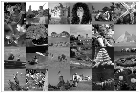
Figure 1.
The 24 test images used in the denoising experiments.
4.1. Low Noise Level
Both the full version and simple versions of our algorithm consistently demonstrated a superior performance in terms of the PSNR and SSIM, compared to the traditional DWT-H/DWT-S/WNLM/NLMW algorithms across very different types of images (Table 1). In terms of PSNR results (Table 1), the simple version of our algorithm achieved significant improvements, with 1.218–5.666 dB, 0.662–5.388 dB, 0.248–3.117 dB, and 0.017–3.025 dB over the DWT-H/DWT-S/WNLM/NLMW algorithm, respectively. The incorporation of wavelet thresholding into the full version of our algorithm further enhanced the denoising performance, leading to an additional improvement of approximately 0.163 dB over the simple version. Regarding the SSIM results (Table 1), the simple version of our algorithm also consistently outperformed the other four wavelet methods, with an average advantage of 0.171, 0.153, 0.086, and 0.083. Our full-version algorithm further enhanced the average SSIM result by approximately 0.004, compared to the simple version.

Table 1.
The PSNR (dB) and SSIM results of six wavelet-denoising algorithms at low noise levels.
Figure 2 demonstrates the denoising visual effects of different algorithms for flower images at a low noise level (). Notably, compared to the four traditional wavelet algorithms, our algorithm demonstrated more convincing improvements in the visual quality of the flower image, especially in reconstructing the edges of the petals and the blurry background. DWT-H and DWT-S over-smooth the image, causing the loss of most details in the flower. NLMW and WNLM manage to retain some structures and details, but noticeable noise remains around the edges of the flower. Compared with these, our algorithms preserve a higher level of detailed information; the reconstruction of the flower exhibits sharper edges, and the overall background appears cleaner. This highlights the enhanced denoising capabilities of our algorithm, especially in terms of producing sharper and more visually pleasing results.
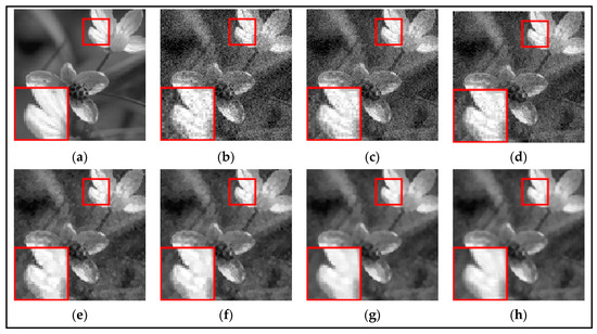
Figure 2.
Denoising performance comparison for a flower image at the noise level . (a) The original image. (b) The noisy image. (c) DWT-H (PSNR = 24.433 dB, SSIM = 0.538). (d) DWT-S (PSNR = 24.701 dB, SSIM = 0.542). (e) WNLM (PSNR = 26.714 dB, SSIM = 0.656). (f) NLMW (PSNR = 27.270 dB, SSIM = 0.680). (g) The simple version of our algorithm (PSNR = 29.346 dB, SSIM = 0.830). (h) The full version of our algorithm (PSNR = 29.481 dB, SSIM = 0.826).
4.2. Middle Noise Level
For middle noise levels ( = 30, 40), the PSNR results (Table 2) demonstrated significant advantages in our simple version over four wavelet algorithms (DWT-H/DWT-S/WNLM/NLMW), with the maximum PSNR differences reaching up to 7.757 dB, 5.985 dB, 3.665 dB, and 2.927 dB, respectively. Moreover, our full version exhibited a superior performance over the simple version in almost all the denoised images. The SSIM results (Table 2) also showed substantial advantages in our algorithms over four traditional wavelet algorithms (DWT-H/DWT-S/WNLM/NLMW). The maximum SSIM differences reached up to 0.491, 0.452, 0.321, and 0.273, respectively. The considerable improvements in PSNR and SSIM values further highlight the effectiveness and potential of our algorithms in handling noise reduction tasks.
Table 2.
The PSNR (dB) and SSIM results of six wavelet-denoising algorithms at middle noise levels.
Figure 3 demonstrates an example of denoising at a middle noise level ( = 30). The DWT-H/DWT-S algorithms yield significantly artifacts, and NLMW and WNLM manage to reduce them in some sense; compared with these algorithms, the simple version of our algorithm exhibited a better performance, by effectively separating the koala’s silhouette from the black background, and producing a clearer image. The full version of our algorithm output the clearest details of the koala silhouette, resulting in a more visually pleasing and aesthetically appealing image. The higher PSNR and SSIM values further support the superiority of our algorithm.
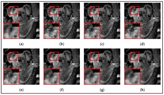
Figure 3.
Denoising performance comparison for the koala image at the noise level = 30. (a) The original image. (b) The noisy image. (c) DWT-H (PSNR = 20.284 dB, SSIM = 0.441). (d) DWT-S (PSNR = 21.745 dB, SSIM = 0.476). (e) WNLM (PSNR = 24.064 dB, SSIM = 0.587). (f) NLMW (PSNR = 25.413 dB, SSIM = 0.675). (g) The simple version of our algorithm (PSNR = 26.225 dB, SSIM = 0.718). (h) The full version of our algorithm (PSNR = 26.258 dB, SSIM = 0.719).
4.3. High Noise Level
At the high noise level, the PSNR/SSIM values of the full and simple versions of our algorithm also outperformed the four known wavelet algorithms (Table 3). At the noise level , the PSNR/SSIM values of the simple version of our algorithm were consistently, on average, 2.415 dB/0.172 higher than the other four algorithms, and the full version of our algorithm, utilizing wavelet thresholding, achieved an additional improvement of approximately 0.449 dB/0.019. Similarly, at the noise level , the PSNR/SSIM values of the simple version of our algorithm were, on average, 1.652 dB/0.1045 higher than four known wavelet algorithms, and the full version of our algorithm achieved an additional 0.151 dB/0.006 improvement. Especially when , all the competing wavelet-denoising algorithms only achieved a low SSIM value, while our algorithm showed a better resilience to a high noise level, by maintaining an SSIM value of 0.5, or even 0.6.
Table 3.
The PSNR (dB) and SSIM results of six wavelet-denoising algorithms at high noise levels.
Figure 4 shows a building image after denoising via six wavelet algorithms at , with a partial zoom in the red box in the lower left corner, to allow for a clearer and more intuitive sense of the denoising effect. It can be seen from the zoomed area that DWT-H and DWT-S brought many ringtone artifacts to the background of the denoised images. As a result, it is difficult to recognize the demarcation and details of the sky and houses. NLMW and WNLM made the image too smooth, leaving some noise at the edge of the chimney. Our algorithm produced clear edges, and restored the basic contours of the dark clouds in the sky.
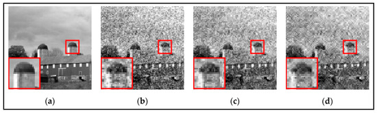
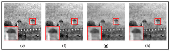
Figure 4.
Denoising performance comparison for the building image at the noise level . (a) The original image. (b) The noisy image. (c) DWT-H (PSNR = 20.002 dB, SSIM = 0.340). (d) DWT-S (PSNR = 20.914 dB, SSIM = 0.350). (e) WNLM (PSNR = 21.937 dB, SSIM = 0.442). (f) NLMW (PSNR = 22.562 dB, SSIM = 0.600). (g) The simple version of our algorithm (PSNR = 23.819 dB, SSIM = 0.657). (h) The full version of our algorithm (PSNR = 24.372 dB, SSIM = 0.688).
4.4. Average Denoising Performance
Table 4 presents the average PSNR and SSIM values for the denoising of the 24 test images at different noise levels. The full version and simple version of our algorithm achieved the best and the second-best denoising results, significantly better than the classic wavelet algorithms (DWT-H, DWT-S) and their extensions (WNLM, NLMW). The full/simple versions of our algorithm outperformed the DWT-H, DWT-S, WNLM, and NLMW algorithms by 4.197/3.946 dB, 3.326/3.075 dB, 2.097/1.846 dB, and 1.162/0.911 dB in terms of average PSNR, and by 0.230/0.219, 0.213/0.202, 0.132/0.121, and 0.085/0.074 in terms of average SSIM. The full and simple versions of our algorithm achieved the smallest mean square error (MSE), with an average reduction of 306.791 compared to other algorithms (Figure 5)
Table 4.
The average PSNR (dB)/SSIM for the denoised images via six wavelet-denoising methods.
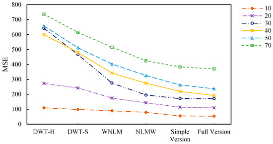
Figure 5.
The average MSE values for the denoised images via six wavelet-denoising methods.
4.5. Denoising Experiments on Kodak24 Dataset
To further demonstrate the feasibility of our improved wavelet-denoising algorithms, we conducted 16 image-denoising experiments images with the higher-resolution Kodak24 (500 × 500) dataset (Figure 6).
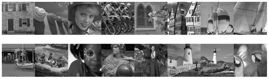
Figure 6.
The 16 test images on Kodak24 used in the denoising experiments.
We present the final PSNR/SSIM results for the denoising of images from the Kodak24 image dataset in Table 5. It is clear that the full version and simple version of our algorithm achieved a better PSNR/SSIM than the other competing algorithms. The full/simple versions of our algorithm outperformed the DWT-H, DWT-S, WNLM, and NLMW by approximately 3.67/3.34 dB, 3.01/2.68 dB, 1.94/1.60 dB, and 1.08/0.82 dB in terms of average PSNR, and by approximately 0.191/0.158, 0.182/0.149, 0.110/0.077, and 0.068/0.038 in terms of average SSIM (Table 5).
Table 5.
The average PSNR (dB)/SSIM for the denoised images on Kodak24 via six wavelet-denoising methods.
4.6. Other Denoising Experiments
We have demonstrated the effectiveness of our improvement in successfully restoring images corrupted by Gaussian noise. However, the practice of image formation often involves a combination of Gaussian and Poisson noises. Hence, we conducted denoising experiments on the images in Figure 1, and considered a mixture of Gaussian noise () and different Poisson noises (λ = 0.4, 5, 10). Across all levels of noise, the full/simple versions of our algorithm consistently exhibited a superior performance compared to the DWT-H, DWT-S, WNLM, and NLMW algorithms (Table 6), manifesting advantages of approximately 3.88/3.68 dB, 3.44/3.24 dB, 2.02/1.83 dB, and 1.28/1.08 dB in terms of average PSNR, respectively, and by 0.252/0.229, 0.231/0.209, 0.149/0.127, and 0.102/0.080 in terms of average SSIM, respectively.
Table 6.
The average PSNR (dB)/SSIM for the denoised images via six wavelet-denoising methods.
5. Conclusions
Compared with classic wavelet algorithms (DWT-H, DWT-S) and their extensions (WNLM, NLMW), our denoising algorithms coupling the wavelet and earth mover’s distance not only yields higher PSNR and SSIM values, but also produces more visually appealing images. Denoising simulations demonstrated that the robustness of our algorithms to various noise intensities highlights its versatility and adaptability to real-world scenarios. The denoising process using our wavelet algorithm does not introduce unwanted artifacts or distortions, resulting in clearer and more aesthetically pleasing results.
The main mechanisms behind our superior denoising performance comprise:
- ➢
- Our algorithm makes full use of not only the wavelet-denoising technique at a local scale, but also the interior similarity and redundancy embedded in the whole image, leading to our superior denoising performance over classic wavelet algorithms (DWT-H, DWT-S). Moreover, the use of joint bilateral filtering as a processing step, which detects high-frequency oscillations inside images, and then preserves image edges, further enhanced the denoising performance.
- ➢
- We used the earth mover’s distance as the similarity measure of small-scale patches of images. The earth mover’s distance (EMD) naturally extends the concept of distance between individual elements to the concept of distance between sets of elements. As the EMD tolerates the distortion of some moving features, it is well recognized as a much more robust clustering measure than the Euclidean distance, leading to our superior denoising performance over WNLM and NLMW, which use the Euclidean distance to measure the similarity.
Denoising experiments on 40 images demonstrated that our algorithm achieved the best and the second-best denoising results, significantly better than classic wavelet algorithms (DWT-H, DWT-S) and their extensions (WNLM, NLMW). While our improvement consistently demonstrates a remarkable performance in contrast to conventional DWT-H, DWT-S, WNLM, and NLMW on various gray images, residual artifacts and subtle discontinuities are possibly discernible along certain boundaries of minor blocks in a few denoised images. Although there is an increasing trend in the application of deep learning in denoising, the deep learning technique must use a huge number of noisy images; the numbers of parameters used in deep learning techniques are very large; and the computation cost is high. However, wavelet-denoising techniques have no such drawbacks. In the future, we intend to couple EMD distance and wavelet techniques into deep-learning-driven denoising models, to reduce the computational cost, and enhance the interpretability. Recently, simple nonlocal similarity measurements are incorporated into classic compressive sensing, and demonstrated the advantage of such an improvement on the denoising of three images (Barbara, Cameraman, and Lena) [38]. Inspired by this approach, we plan to use the EMD distance to further enhance the denoising performance of compressive sensing in the future. Meanwhile, our future efforts will expand our algorithm’s scope, to cover color image denoising, image segmentation, focal point detection, and image deblurring.
Author Contributions
Z.Z. and X.X. are co-first author. Conceptualization, Z.Z.; Methodology, Z.Z.; Software, X.X.; Validation, X.X.; Formal analysis, Z.Z., X.X. and M.J.C.C.; Investigation, Z.Z.; Data curation, X.X.; Writing—original draft, Z.Z. and X.X.; Writing—review & editing, Z.Z. and M.J.C.C.; Visualization, X.X.; Supervision, Z.Z. All authors have read and agreed to the published version of the manuscript.
Funding
The corresponding author was supported by the European Commission Horizon 2020 Framework Program No. 861584 and the Taishan Distinguished Professor Fund No. 20190910.
Institutional Review Board Statement
Not applicable.
Informed Consent Statement
Not applicable.
Data Availability Statement
Not applicable.
Conflicts of Interest
The authors declare no conflict of interest.
References
- Meyer, Y.; Coifman, R.; Salinger, D. Wavelets: Calderón-Zygmund and Multilinear Operators; Cambridge University Press: Cambridge, UK, 1997. [Google Scholar]
- Mallat, S. A Wavelet Tour of Signal Processing: The Sparse Way; Academic Press: Cambridge, MA, USA, 2008. [Google Scholar]
- Daubechies, I. Ten Lectures on Wavelets; Society for Industrial and Applied Mathematics: Philadelphia, PA, USA, 1992. [Google Scholar]
- Gurkahraman, K.; Karakis, R.; Takci, H. A Novel Color Image Watermarking Method with Adaptive Scaling Factor Using Similarity-Based Edge Region. Tech. Sci. Press 2023, 47, 55–77. [Google Scholar] [CrossRef]
- Gowthami, V.; Bagan, K.B.; Pushpa, S.E.P. A novel approach towards high-performance image compression using multilevel wavelet transformation for heterogeneous datasets. J. Supercomput. 2023, 79, 2488–2518. [Google Scholar] [CrossRef]
- Syed, S.H.; Muralidharan, V. Feature extraction using Discrete Wavelet Transform for fault classification of planetary gearbox—A comparative study. Appl. Acoust. 2022, 188, 108572. [Google Scholar] [CrossRef]
- Samantaray, A.K.; Gorre, P.; Sahoo, P.K. Design of CSD based Bi-orthogonal Wavelet Filter Bank for Medical Image Retrieval. Adv. Electr. Eng. Electron. Energy 2023, 5, 100242. [Google Scholar] [CrossRef]
- Gonzalez, R.C.; Woods, R.E. Digital Image Processing, 3rd ed.; Prentice Hall Press: Englewod Cliffs, NJ, USA, 2007. [Google Scholar]
- Huang, T.; Yang, G.; Tang, G. A fast two-dimensional median filtering algorithm. IEEE Trans. Acoustic. Speech. Signal Process. 1979, 27, 13–18. [Google Scholar] [CrossRef]
- Tomasi, C.; Manduchi, R. Stereo matching as a nearest-neighbor problem. IEEE Trans. Pattern Anal. Mach. Intell. 1998, 20, 333–340. [Google Scholar] [CrossRef]
- Lee, J.S. Digital image enhancement and noise filtering by use of local statics. IEEE Trans. Pattern Anal. Mach. Intell. 2009, 2, 165–168. [Google Scholar]
- Perona, P.; Malik, J. Scale-space and edge detection using anisotropic diffusion. IEEE Trans. Pattern Anal. Mach. Intell. 2002, 12, 629–639. [Google Scholar] [CrossRef]
- Elad, M. On the origin of the bilateral filter and ways to improve it. Image Process. IEEE Trans. 2002, 11, 1141–1151. [Google Scholar] [CrossRef]
- Rabbani, H. Image denoising in steerable pyramid domain based on a local Laplace prior. Pattern Recognit. 2009, 42, 2181–2193. [Google Scholar] [CrossRef]
- Srivastava, M.; Anderson, C.L.; Freed, J.H. A New Wavelet Denoising Method for Selecting Decomposition Levels and Noise Thresholds. IEEE Access 2016, 4, 3862–3877. [Google Scholar] [CrossRef]
- Johnstone, M.; Silverman, B.W. Wavelet Threshold Estimators for Data with Correlated Noise. J. R. Stat. Soc. 1997, 59, 319–351. [Google Scholar] [CrossRef]
- Donoho, D.L.; Johnstone, I.M. Adapting to unknown smoothness via wavelet shrinkage. J. Am. Stat. Assoc. 1995, 90, 1200–1224. [Google Scholar] [CrossRef]
- Luiser, F.; Blu, T.; Unser, M. A new SURE approach to image denoising: Inters ale orthonormal wavelet thresholding. IEEE Trans Image Process. 2007, 9, 593–606. [Google Scholar] [CrossRef]
- Chang, S.G.; Yu, B.; Vetterli, M. Adaptive wavelet thresholding for image denoising and compression. IEEE Trans. Image Process 2000, 9, 1532–1546. [Google Scholar] [CrossRef]
- Blu, T.; Luisier, F. The SURE-LET approach to image denoising. IEEE Trans. Image Process 2007, 16, 2778–2786. [Google Scholar] [CrossRef]
- Chen, G.Y.; Bui, T.D.; Krzyzak, A. Image denoising with neighbor dependency and customized wavelet and threshold. Pattern Recognit. 2005, 38, 115–124. [Google Scholar] [CrossRef]
- Zhou, D.; Cheng, W. Image denoising with an optimal threshold and neighboring window. Pattern Recognit. 2008, 29, 1694–1697. [Google Scholar]
- Yi, T.H.; Li, H.N.; Zhao, X.Y. Noise Smoothing for Structural Vibration Test Signals Using an Improved Wavelet Thresholding Technique. Sensors 2012, 12, 11205–11220. [Google Scholar] [CrossRef]
- Liu, H.; You, Y.; Li, S.; He, D.; Sun, J.; Wang, J.; Hou, D. Denoising of Laser Self-Mixing Interference by Improved Wavelet Threshold for High Performance of Displacement Reconstruction. Photonics 2023, 10, 943. [Google Scholar] [CrossRef]
- Iqbal, M.Z.; Ghafoor, A.; Siddiqui, A.M. Satellite image resolution enhancement using dual-tree complex wavelet transform and nonlocal means. IEEE Geosci. Remote Sens. Lett. 2012, 10, 451–455. [Google Scholar] [CrossRef]
- Diwakar, M.; Kumar, M. CT image denoising using NLM and correlation-based wavelet packet thresholding. IET Image Process. 2018, 12, 708–715. [Google Scholar] [CrossRef]
- Diwakar, M.; Kumar, P.; Singh, A.K. CT image denoising using NLM and its method noise thresholding. Multimed. Tools Appl. 2020, 79, 14449–14464. [Google Scholar] [CrossRef]
- Suresh, K.V. An improved image denoising using wavelet transform. In Proceedings of the 2015 International Conference on Trends in Automation, Communications and Computing Technology, I-TACT-15, Bangalore, India, 21–22 December 2015. [Google Scholar]
- Singh, K.; Ranade, S.K.; Singh, C. Comparative performance analysis of various wavelet and nonlocal means-based approaches for image denoising. OPTIK-Int. J. Light Electron Opt. 2017, 131, 423–437. [Google Scholar] [CrossRef]
- Ye, S.; Mei, Y. Super resolution image reconstruction based on wavelet transform and non-local means. J. Comput. Appl. 2014, 34, 1182–1186. [Google Scholar]
- Rubner, Y.; Tomasi, C.; Guibas, L.J. The Earth Mover’s Distance as a Metric for Image Retrieval. Int. J. Comput. Vis. 2000, 40, 99–121. [Google Scholar] [CrossRef]
- Basha, B.; Nandi, D.; Kaur, K.N.; Arambam, P.; Gupta, S.; Segan, M.; Ranjan, P.; Kaul, U.; Janardhanan, R. Earth Mover’s Distance-Based Automated Disease Tagging of Indian ECGs. In Machine Learning in Information and Communication Technology: Proceedings of ICICT 2021, SMIT; Springer Nature Singapore: Singapore, 2023; Volume 498, pp. 3–19. [Google Scholar]
- Zhang, L.; Zhang, P. Research on aesthetic models based on neural architecture search. J. Intell. Fuzzy Syst. 2021, 8, 1–15. [Google Scholar] [CrossRef]
- Ling, Y.; Zhong, Z.; Cao, D.; Luo, Z.; Lin, Y.; Li, S.; Sebe, N. Cross-modality earth mover’s distance for visible thermal person re-identification. In Proceedings of the Computer Vision and Pattern Recognition, New Orleans, LA, USA, 18–24 June 2022; Volume 14. [Google Scholar]
- Yu, H.; Zhao, L.; Wang, H. Image Denoising Using Triradiate Shrinkage Filter in the Wavelet Domain and Joint Bilateral Filter in the Spatial Domain. IEEE Trans. Image Process. 2009, 18, 2364–2369. [Google Scholar]
- Karthikeyan, P.; Vasuki, S. Multiresolution joint bilateral filtering with modified adaptive shrinkage for image denoising. Multimed. Tools Appl. 2016, 75, 16135–16152. [Google Scholar]
- Zhang, M.; Gunturk, B.K. Multiresolution Bilateral Filtering for Image Denoising. IEEE Trans. Image Process. 2008, 17, 2324–2333. [Google Scholar] [CrossRef]
- Mahdaoui, A.E.; Ouahabi, A.; Moulay, M.S. Image Denoising Using a Compressive Sensing Approach Based on Regularization Constraints. Sensors 2022, 22, 2199. [Google Scholar] [CrossRef] [PubMed]
Disclaimer/Publisher’s Note: The statements, opinions and data contained in all publications are solely those of the individual author(s) and contributor(s) and not of MDPI and/or the editor(s). MDPI and/or the editor(s) disclaim responsibility for any injury to people or property resulting from any ideas, methods, instructions or products referred to in the content. |
© 2023 by the authors. Licensee MDPI, Basel, Switzerland. This article is an open access article distributed under the terms and conditions of the Creative Commons Attribution (CC BY) license (https://creativecommons.org/licenses/by/4.0/).