Abstract
As the Artificial Intelligence of Things (AIOT) and ubiquitous sensing technologies have been leaping forward, numerous scholars have placed a greater focus on the use of Impulse Radio Ultra-Wide Band (IR-UWB) radar signals for Region of Interest (ROI) population estimation. To address the problem concerning the fact that existing algorithms or models cannot accurately detect the number of people counted in ROI from low signal-to-noise ratio (SNR) received signals, an effective 1DCNN-LSTM model was proposed in this study to accurately detect the number of targets even in low-SNR environments with considerable people. First, human-induced excess kurtosis was detected by setting a threshold using the optimized CLEAN algorithm. Next, the preprocessed IR-UWB radar signal pulses were bundled into frames, and the resulting peaks were grouped to develop feature vectors. Subsequently, the sample set was trained based on the 1DCNN-LSTM algorithm neural network structure. In this study, the IR-UWB radar signal data were acquired from different real environments with different numbers of subjects (0–10). As indicated by the experimental results, the average accuracy of the proposed 1DCNN-LSTM model for the recognition of people counting reached 86.66% at ROI. In general, a high-accuracy, low-complexity, and high-robustness solution in IR-UWB radar people counting was presented in this study.
1. Introduction
As AIOT [1] and pervasive sensing technology have been rapidly advancing, the development of smart homes, the smart industry, and smart security fields has been boosted over the past few years. Under this context, several problems are triggered (e.g., abnormal crowd flow leading to stampede events, inaccurate business analysis in critical areas, as well as low level of indoor security). Accordingly, numerous scholars worldwide have used sensors to analyze the people counting [2,3] and population density [4] in a fixed area ROI over the past few years. In the literature [5], the video image extraction of features was adopted to address the problem of people counting. However, the critical disadvantage of video-image-based algorithms is that they can be easily affected by lighting conditions, viewpoint diversity, and spatial complexity, and their performance fluctuates wildly. Under extreme conditions (e.g., fog and smoke), video-image-based algorithms exhibit poor performance or even fail to work; they are prone to problems regarding the disclosure of personal privacy. Moreover, most video-image-based algorithms collect high-resolution HD images or videos as the training samples, and the algorithms consume huge memory and computational space. Thus, researchers have placed their focus on Radio Frequency (RF)−based algorithms [6,7]. RF-based people counting methods [8] are mainly: WiFi-based people counting methods and Radio Frequency Identification (RFID)−based people counting methods. WiFi-based people counting methods include the following two: on the one hand, there is the use of RSSI [9] in WiFi for people counting. On the other hand, it is categorized using a Channel State Information (CSI) [10] subcarrier variation rule of the WiFi physical layer. However, since WiFi signals can be easily interfered with via the multipath effect, it cannot indicate the subject information timely and accurately, leading to the dilemma of low recognition accuracy. An RFID-based [7,8] people counting method is not convenient for daily use and maintenance due to the considerable number of RF sensor devices required. Besides RF-based people counting methods, there are also detection methods using (Passive Infrared Detectors) PIR [11] and thermal imaging-based techniques [12]. PIR-based detection methods are simple in principle and in terms of equipment and exhibit low algorithmic complexity; however, they are susceptible to detection failures under the effect of the surrounding temperature. The advantage of the thermal imaging-based detection method is that it can be applied to low-light environments. However, the disadvantage is that it is still as susceptible to the effect of ambient temperature as the PIR-based detection method. Furthermore, thermal imaging-based detection methods consume more computational resources since the algorithms exhibit higher complexity.
Ultra-Wide Band (UWB) technology complies with the communication band of 3.1–10.6 GHz, which was mandated by the U.S. FCC in 2002 [13]. UWB uses a higher and wider frequency band compared to other communication technologies. The popular Bluetooth and WiFi communications use a narrow bandwidth of 2.4 GHz and 5 GHz, respectively, and are very high power, as shown in Figure 1. IR-UWB radar transmits data using non-positive-wave pulses in the nanosecond (ns) to picosecond (ps) range, which occupies bandwidths up to several gigahertz so that the maximum data rate can be up to a few hundred meters per second. It can be seen that the use of pulse radio technology in the physical layer of the air interface of UWB technology is used to increase the data transmission rate of the physical layer. A comparison of conventional narrowband communication systems with the transceivers of IR-UWB shows a clear difference in the way the two technologies are implemented. Narrowband systems generally use sinusoidal carrier modulation to realize spectrum migration, the channel transmits the RF-tuned signal, and the receiver needs to demodulate after down-conversion step by step to recover the original information. In contrast, IR-UWB directly sends broadband narrow pulses after spectrum shaping. The channel transmits baseband signals, and the receiver is mainly a correlation detector, which is much simpler in structure than the traditional narrowband communication system. IR-UWB technology solves the significant problems related to propagation that plague conventional wireless technology and has the advantages of insensitivity to channel fading, low power spectral density of the transmitted signal, low system complexity, and centimeter-level positioning accuracy. Therefore, UWB technology offers low strength, high discrimination, excellent non-contact performance, and anti-interference performance. In recent years, applications based on UWB technology have sprung up, such as their use in the detection of physical signs such as breathing and heartbeat [14], non-contact subject target trajectory recording [15], and target location determination in large indoor scenes [16].
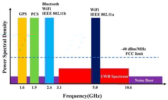
Figure 1.
Frequency band distribution map for different technologies.
In recent years, many scholars have focused on people counting methods based on pulsed radar [17] as well as Frequency Modulated Continuous Wave (FMCW) radar [18] because of their low or even negligible influence in terms of light or ambient temperatures, their high resolution in terms of people or objects, and their lack of related issues such as those relating to personal privacy. IR-UWB radar-based people counting methods generally have the following two branches, one is Line of Interest (LOI), which is the detection of people standing on the same line at a certain fixed angle, for example, in [19,20]. The authors used IR-UWB radar sensors to explore the LOI of person counting on a certain line people counting. The second is ROI, i.e., people counting on a fixed size for a fixed region, which is also the concern of the research in this paper. In [21], the authors use an iterative algorithm to detect the local maxima of IR-UWB radar signals to count people. In the paper [22], the authors simulate the theoretical model of UWB signals. In [23], the authors proposed an algorithm based on principal clustering to analyze the distribution of selected magnitudes with distance and number of people. In papers [24,25], the authors detect each signal caused by a person from the received radar echoes, thus determining the number of people. However, due to the influence of the surrounding environment, the received radar echoes are often interspersed with and contain clutter caused by multipath effects. This detection method is not accurate in counting the number of individuals.
Many scholars have been working on problems related to electromagnetic interference, scattering, and multipath effects in recent years. The article [26] investigates the problem of electromagnetic solid interference suppression without a priori information in non-cooperative scenarios, the issue of near-field EMI suppression is investigated, and the proposed algorithm effectively suppresses strong EMI without a priori knowledge while effectively capturing the target signal. In the article [27], the authors proposed a method to effectively solve the problem of near-area electromagnetic scattering of scatterers under external field irradiation. The method is based on the Helmholtz equation discretized using the finite element method. In dealing with the reverberation and interference fields of the signal, the authors [28] have combined the minimum variance distortionless response (MVDR) beamformer with Multi-Channel Linear Prediction (MCLP) to achieve active noise reduction. In order to effectively deal with multipath propagation of signals, the article [29] addresses the reverberation of radar echo data. It proposes an alternative to conventional reverberation estimation for use in time-frequency sequence to deal with reverberation. At the same time, in order to solve the multipath effect of IR-UWB radar echoes, the authors in [23] used the Probabilistic Model (PM) to analyze the variation rule of amplitude with the distance of the selected radar echoes to determine the number of individuals in the target area. Still, this algorithm is not applicable to cases where there are too many people in the target area. The authors in [30] proposed an algorithm to count the number of individuals in the target area under the condition of there being too many persons in an area using image feature extraction of 2D signals. However, this algorithm is unable to do anything for IR-UWB radar signals with low SNR.
To address the complexity of the current domestic and international research on the analysis of IR-UWB radar signals, it is difficult to accurately detect the number of people counted in the ROI from low SNR signals using the existing solutions. For this reason, in this study, an effective 1DCNN-LSTM algorithm is proposed to accurately detect the number of targets, even under the conditions of low SNR environments with considerable people. In the literature [31], Convolutional Neural Network (CNNs) [32] techniques have been adopted for the spontaneous filtering of noisy signals from the received signals and images while extracting effective features by constructing a model. Existing research suggested that CNNs apply to the extraction of features with non-temporal dependencies [33] or features that show more significant local differences. However, the received signals were time series with high time dependencies, such that the CNN technique should be adopted alone.
Long Short-Term Memory (LSTM) networks refer to a particular version of RNN that contain cyclic feedback designed to process time series [34]. Thus, the LSTM layer is capable of encoding information regarding class-specific features across time [35]. Given this finding, a model architecture combining CNN and LSTM networks was proposed in this study, considering the temporal characteristics of IR-UWB radar signals.
The remaining parts of this study are given below. The IR-UWB radar signals are modeled in Section 2. Section 3 describes the proposed people counting classification model in detail. The performance assessment of the experiments and the analysis of the results are placed in Section 4 of the paper. The last section summarizes the work of this study.
2. Signal Preprocessing
2.1. IR-UWB Radar Principle
Due to the presence of various interfering information, noise, and multipath effects in all existing experimental environments, the raw echoes received by IR-UWB radar will cover considerable useless information. Accordingly, extracting useful information from the raw echoes containing many interfering signals and clutter signals for the estimation of the number of people is a major challenge in this study. To simplify the experimental model for quantitative analysis and to focus on the improvement of the experimental scheme and algorithm, the experimental object is in the ROI area. The IR-UWB transmitter is located on the top of the device, and the receiver is placed under the device. The experimental schematic is shown in Figure 2.
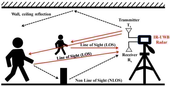
Figure 2.
Experimental schematic diagram.
In this study, the sampling of IR-UWB signals conformed to time series, i.e., on time-domain information. The sampling comprised two parts: (1) sampling the time-domain information of the propagation of a single echo pulse signal from the IR-UWB radar, which was termed fast-time sampling, and (2) defining a time axis for the sequential order of the pulse signals received by the IR-UWB radar, which was termed slow-time sampling. The IR-UWB radar emitted a pulse signal, , with the following expression [36]:
where denotes the amplitude value of the IR-UWB signal, represents the effective width of the pulse (−10 db), expresses the frequency of the carrier, and is the fast time-domain time under a single slow time sample. The IR-UWB radar transmitter will receive the pulse signal in Equation (1) through a series of reflections, and the analog signal will be converted into a digital signal. The received signal of the converted digital is given below:
In the given equation, the quantities represented by and correspond to the noise levels in the subject and the environment, respectively. Moreover, and represent the multipath effect noise signals arising from the reflected signal of the ith subject target and the ith target, respectively. expresses the value of the amplitude of the IR-UWB radar signal emitted by the subject. Furthermore, and denote the effect of multipath effects from the environment on the IR-UWB radar signal and the amplitude of the clutter signal, respectively. represents the sampling index point in the first case of the frame, while represents the sequential value of the slow time sampling. denotes the Gaussian noise value in each frame 1 case. For the proposed specific IR-UWB radar system, represents the number of samples, and the respective slow-time sampling frame comprised fast-time sampling points, which is denoted as . By obtaining the above-mentioned frames, the temporal variation of the subject target can be represented using a cumulative two-dimensional signal matrix.
Following Equation (2), can be obtained. In the following, we will first perform an integration of the sampling points along the fast time series, and every bin of was integrated into one interval. Thus, the fast-time samples of were divided into intervals, with denoting downward rounding. Next, the maximum value of the bins was used for assignment. The signal after the above processing can be expressed as:
where . To effectively solve the static clutter in the environment, the running average method [21] was adopted to eliminate in Equation (2). For the IR-UWB radar received signals in Equation (2), the human signals were masked by clutter signals arising from reflections from non-human objects (e.g., walls, ceilings, and columns). Accordingly, the clutter was characterized by less motion, thus becoming less time-varying than human signals. The running average method refers to a technique that employs the above-described characteristics to suppress the clutter signals with less time-varying per time, which is expressed in Equation (4):
where denotes the noise signal obtained from the kth pulse. denotes the original IR-UWB signal, excluding the noise signal arising from the environment, and is a weighting factor that determines how many signals with small variations over time are considered clutter. The clutter signal of the second pulse can be calculated using the clutter signal of the previous pulse and the current received pulse signal.
2.2. Clutter Suppression
After using the running average method on the IR-UWB signal, to further improve the SNR and suppress the radar clutter, the sampled signal in this study was filtered as follows. Work from the literature [37] highlighted that the experimental environment (including temperature and humidity values; dielectric constant), multipath effect, and so forth, will affect IR-UWB signals; therefore, a Butterworth filter was adopted to reduce the noise of IR-UWB signals, and the transfer function can be expressed as follows.
where denotes the frequency value of the cutoff and represents the filter order. In this study, we considered the complexity of the algorithm as well as the overall performance of the filters. Through the feedback of the experimental results two fifth-order filters were selected, i.e., set to 5. Next, the normalized cutoff frequency was given.
is the frequency during fast-time sampling. We obtain the following equation after performing the filtering operation on the slow time sample point on the fast time sample .
where means the order of the low pass filter is 5. Similarly, means the order of the high pass filter is also set to 5. and denote the filter coefficients. Moreover, in this study, we adopted a smoothing filter, which is more commonly used, to suppress non-stationary noise signals.
where is a value from 1 to , and denotes downward rounding. To enhance the SNR of the IR-UWB signals while suppressing the non-stationary noise signals, seven values are averaged over the slow time sampling interval, i.e., is set to 7.
2.3. Adaptive Gain Control
Due to the presence of distance-dependent signal attenuation in IR-UWB radar signals, the reflected signals turn out to be weaker when a person’s position is far away from the sensors. Thus, in the proposed people counting system, the above problem is compensated for by using the Adaptive Gain Control (AGC) process to minimize the distance dependence of the signal. The AGC process is conducted by multiplying with the distance-compensated signal , as expressed in Equation (9).
where denotes the th pulse passing through the final preprocessing of the AGC process. indicates the velocity of light, and is a constant that controls the degree of attenuation of the signal strength. Excess kurtosis can be used to extract non-Gaussian signals and to also determine their position in frequency. Excess kurtosis is shown in the following equation:
where denotes the second-order center distance of the overall sample. Likewise, is fourth-order. represents the expectation of the sample. Figure 3a,b present the raw and preprocessed IR-UWB radar signals received concerning three people in the ROI region, respectively. As depicted in Figure 3, the signals of the people turned out to be more prominent when the raw IR-UWB radar signals were preprocessed, as presented in Figure 3b. Lastly, the preprocessed IR-UWB radar signal comprised human signals, multipath signals, and noise signals. The above-mentioned multipath and noise signals interfered with accurate coefficient estimation and require further processing to resolve them.
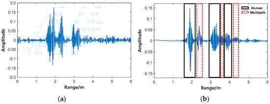
Figure 3.
Comparison of signal processing with three people in ROI. (a) IR-UWB radar signal before processing. (b) IR-UWB radar signal after processing.
3. Proposed Method
In the present section, the process of bundling preprocessed signal pulses into frames and then forming a feature vector from the respective formed frame is illustrated. First, artificially induced signal peaks were detected using a modified CLEAN algorithm by changing the threshold value. Next, the formed peaks were grouped to form a feature vector. Lastly, the feature vector was calculated for the respective number of people from 0 to 10, and the classifier was trained using the created database as the training data.
3.1. Improved CLEAN Algorithm for Peak Detection
The effect of multipath and noise signals present in the preprocessed signal should be minimized to ensure the accurate estimation of person counts. Accordingly, it is imperative to effectively suppress the above-described unwanted signals and only extract the signals corresponding to people. The CLEAN algorithm was modified to detect only the people’s peaks in the input signal [21]. The algorithm detected human peaks by removing multiplexed signals located in the vicinity of the human signal and treating signals below a certain intensity as noise. The detailed algorithm is expressed as follows (Algorithm 1).
| Algorithm 1 Improved CLEAN algorithm based on IR-UWB Radar signal threshold |
| 1: Procedure |
| 2: ←Preprocessed signal |
| 3: ←Noise threshold |
| 4: ←Multipath threshold |
| 5: ←Output signal |
| 6: calculate |
| 7: do |
| 8: calculate |
| 9: if Remove multipath |
| 10: then |
| 11: end if |
| 12: while Remove noise |
| 13: return |
| 14: End procedure |
In the above-mentioned process, the critical point is to remove the noise signal and multipath signal through proper thresholding noise threshold and multipath threshold . However, in the case of people moving randomly, it is almost impossible to set the optimal thresholds to enable accurate extraction of human signals. As depicted in Figure 4, increasing removed more noisy signals, whereas it also removed human signals with small signal strength. On the other hand, decreasing increased the probability of detecting small human signals and the probability of detecting noisy signals. For multipath signals, increasing removed multipath signals more efficiently, whereas signals from humans located in close proximity cannot be separated. In contrast, decreasing can accurately separate people in close proximity, but the multipath signal was also detected. In brief, the trade-off between increasing and decreasing the values of and makes it difficult to set the optimal value.
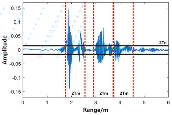
Figure 4.
IR-UWB Radar Signal threshold setting diagram.
3.2. Feature Vector Extraction
The proposed algorithm used multiple thresholds to extract human signals instead of a single threshold. Moreover, it addressed the above problem by removing the redundant information generated in the process through a later dimensionality reduction operation. First, the human signal was extracted by changing to (, , , ) in accordance with the noise signal threshold . Moreover, the extraction algorithm was performed by changing to (, , , ) following the average multipath signal threshold . Through the above-mentioned process, human signals can be extracted for a wide variety of cases. Lastly, the extraction algorithm was performed a total of 25 times.
Based on the human signals extracted by changing the threshold, the algorithm formed a frame using the signals in the slow time direction and then extracted the feature vector from it. Given , the th slow time-indexed frame is expressed as shown in Equation (11).
where denotes the person signal extracted using the threshold . represents the slow time index, and expresses the fast time index. denotes the pulse size of the sampling received signal.
A signal variable depending entirely on the number of people can be defined based on each of the formed frames. First, with the increase in the number of people, the number of peaks in the extracted signal increases. Thus, the number of peaks in the frame excluding 0 was calculated to define , as expressed in Equation (12). Second, as the number of people increased, the signal peaks increased with time. Accordingly, after the distance value was fixed, the variance value of the signal peaks over time was calculated, and the average of each variance value obtained by distance was calculated to define , as shown in Equation (13). Lastly, a frame-by-frame feature vector can be formed by calculating and for the respective frame.
Since human signals were acquired in a total of 25 threshold combinations, 25 frames were acquired for the respective impulse signal. In addition, following the above equation, two feature variables were calculated per frame, such that a total of 50 feature variables can be calculated from the signal. Thus, a feature vector can be formed with the respective feature variable as an element, as defined by the following equation.
where
Lastly, from each frames of data, a feature vector can be formed, i.e., a training database can be built, as expressed in Equation (16).
3.3. 1DCNN-LSTM Model
In general, CNNs comprise multiple convolutional layers adopted to distinguish and extract features, and pooling operations are performed after the convolutional operations. CNNs have been extensively employed in feature extraction and classified into 1-dimensional 1DCNN and 2-dimensional 2DCNN following the dimensionality of the input sequence [38]. Usually, 2DCNN is primarily applied to feature extraction of images, e.g., in the literature [39,40], whereas IR-UWB radar echo signals belong to one-dimensional time series signals, such that 1DCNN more significantly applies to 2DCNN to represent IR-UWB radar signals. Moreover, the model of 1DCNN is more straightforward than that of 2DCNN, and 1DCNN exhibits lower computational complexity [41]. Furthermore, if 2DCNN is used to process time-series IR-UWB radar echo signals, additional signal transformations are required. Thus, 1DCNN was selected instead of 2DCNN.
Accordingly, since IR-UWB signals present time-varying and noise components that should be different from the practical target signals, the idea of LSTM networks was adopted. In this study, a first framework was proposed, utilizing IR-UWB signals from LSTM networks to differentiate between perceived subject targets in ROI ambient environments as well as multipath effects and noise. The proposed deep learning network architecture (Figure 5) incorporated a 1DCNN-LSTM design. It covered a wide variety of components (e.g., a Batch Norm for network stabilization during training, three convolutional layers, two maximal pooling layers, a bi-directional LSTM layer, as well as a fully connected layer).
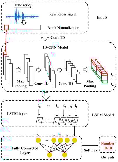
Figure 5.
The proposed 1DCNN-LSTM architecture for deep learning networks.
In this study, a nested 11-fold cross-validation method was adopted for hyperparameter optimization. The training set was divided into 11 sub-training sets of the same size according to the number of people from 0 to 10. The 11-fold cross-cycle validation is performed outside the nested sets, where 6 sub-training sets are used for training, and the remaining 5 are test sets for testing purposes. Moreover, cross-cycle validation with the same external is performed inside each nesting. Lastly, we set the hyperparameters via the use of Cohen’s kappa values. In each CNN layer, as shown in Figure 5, the input layer of the CNN layer is set to have a fixed step size of 2 and the same for the kernel. In the proposed 1DCNN-LSTM model, the Adam optimizer is used for the optimization operation [42], while the Henormal initializer is chosen for the initialization of training [43]. In this study, the earliest patient stop is set to 15, and the learning rate is 0.002, while the loss function uses the cross-entropy function. The proposed 1DCNN-LSTM model is trained in Python 3.6 with the Keras framework [44], while the open-source training platform TensorFlow [45] is used. In the proposed 1DCNN-LSTM model, the features are continuously extracted layer by layer from the lower to the higher-level features. Lastly, the higher-level features are used for training, i.e., to reach the input layer of Softmax. Note that in the convolutional layer, each unit is subjected to a batch normalization and activation function layer after the convolutional operation to improve the overall robustness and performance of the network in the proposed 1DCNN-LSTM model [46]. In this study, the total number of classes was set to 11 based on the size of the number of people in the ROI region (0–10), so the size of the output layer of the model is 11. Table 1 shows the 1DCNN-LSTM architecture of the proposed deep learning network.

Table 1.
The proposed 1DCNN-LSTM architecture for deep learning networks.
CNNs use local filters for convolution operations, i.e., they use local submatrices and local filters for inner product operations, and the convolution layer will use multiple such local filters to compute multiple output matrices, which are referred to as feature layers. For the proposed method, is the input sequence of the IR-UWB radar, is the value of each window after data segmentation, and its input data are defined as:
Additionally, the detailed operation of the convolutional layer is as follows:
where denotes the amount of layers of convolution, represents the amount of feature map layers, expresses the activation function, denotes the bias term of the th feature layer, represents the number of convolution kernels, i.e., the number of local filters, is the output of the th layer, which for the first layer is the initial input data of the model, and expresses the value of the weights of the th feature map of each layer.
The activation function takes on critical significance in artificial neural network modeling. It can learn and gain insights into very complex and nonlinear functions, such that the activation function layer was introduced to the proposed model. For the proposed 1DCNN-LSTM model, the activation function in the hidden layer used the ReLu function in Equation (19), such that the gradient descent or vanishing problem can be effectively avoided [47], which is expressed as:
The Softmax function serves as the activation function for the output layer, expressed as follows.
In Equation (20), the vectors and denote the subject target’s output and predicted output, respectively. denotes the learning rate, and expresses the value of the gradient operator. In this study, cross entropy was selected as the loss function, denoted as , for the 1DCNN-LSTM model. This loss function was utilized in relation to the parameter set .
where the cross entropy denotes the difference between the amount of information contained in and the amount of information contained in . The smaller its value, the closer the number of people the proposed model estimates to the practical value.
Since the received IR-UWB radar signals were time-series data, LSTM is recommended [48]. LSTM is capable of avoiding the situation of long-term dependencies using RNN networks. Moreover, the LSTM network exhibited high resolution in processing time-series datasets. The structure of the LSTM cell is presented in Figure 6, and the LSTM unit is expressed by Equation (22):
where represents the input sequence denoted as , where expresses the temporal length of the input sequence. represents the unit state of the LSTM input gate, whereas expresses the unit state of the output gate. Moreover, denotes the unit state of the forget gate, while represents the state of the storage unit. The unit output of the LSTM unit is denoted as , and the final output sequence is expressed as . denotes the Hyperbolic Tangent function. denotes the Sigmoid function. and denote the input weights and bias vectors regarding the inputs of the LSTM unit, respectively.
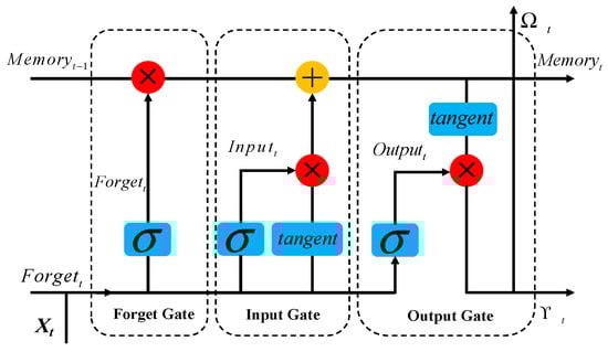
Figure 6.
Architecture of LSTM unit.
4. Experimental Results and Analysis
A comprehensive set of experiments was performed to assess the efficacy of the proposed 1DCNN-LSTM-based model. In this regard, we collected data in a meticulous manner and presented a detailed account of the data collection process. Furthermore, we provide an analysis of the results obtained from processing the collected data, shedding light on the outcomes achieved through the proposed model. To verify the performance of the proposed system, this section elaborates on the performance parameters such as data collection, accuracy, confusion matrix, and ROC curves, and we also compare the experimental performance of different algorithms.
4.1. Data Collection
For the data collection process in this study, an IR-UWB radar sensor provided by Xethru was employed. The specific model employed was the X4M02, and its physical diagram is displayed in Figure 7. Detailed specifications of the radar sensor can be found in Table 2. During the experiment, the IR-UWB radar sensor was mounted on a tripod at a height of 1.5 m above the ground. Additionally, a laptop computer was connected to facilitate data acquisition.
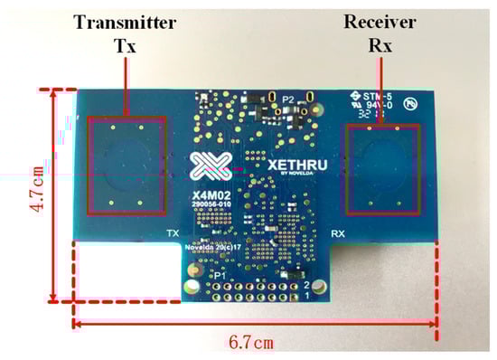
Figure 7.
IR-UWB radar diagram.
Table 2.
IR-UWB radar system parameters.
Experiments were performed in a typical scenario. The experiments were performed in two different locations, the first in an open outdoor environment (Figure 8a) and the second in a room with walls, ceiling, and so forth on all sides, which was termed an indoor open environment (Figure 8b). The experiments were performed in a right-angled sector space with a radius of 6 m and a center angle of 90°. An X4M02 radar was mounted at a height of 1.5 m at the position of the sector apex. The experiment was performed by 10 volunteers, including six males and four females. To protect the privacy of the volunteers, we did not disclose information (e.g., volunteer photographs) in the picture. The information on the volunteers is listed in Table 3.
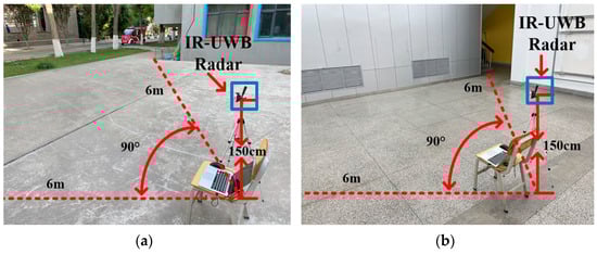
Figure 8.
Diagram of real experimental scene. (a) Outdoor open environment. (b) Indoor open environment.
Table 3.
Physical information of volunteers.
Next, radar signals were acquired for the respective number of people with a minimum of 0 and a maximum of 10 to form a feature vector database and train an IDCNN-LSTM classifier. Thus, with the aim of recording the absolute situation and relative situation cases as comprehensively as possible for the people, the volunteers fell into the ROI detection area. The volunteers’ movements were completely randomized (e.g., standing, swaying, and walking), i.e., each person was allowed to move freely within the experimental space to try to be as dispersed as possible. Each person was given 24,576 received pulses for training purposes, while the X4M02 radar can transmit and receive 48 pulses per second, thus creating one frame for every 48 pulses, forming 512 frames. The training and test datasets were created using a sliding method along the slow time axis. To be specific, an extraction was performed, and then five frames were followed and slid back to initiate a new extraction. The above-described method was adopted to form the training and test datasets. Thus, the 300 s raw data produced 60 samples. The respective case ranged from 0 to 10 people. Lastly, a dataset was generated containing 1024 samples. Due to the partitioning of the dataset for the respective case, the data of 768 samples were applied to the IDCNN-LSTM classifier, and the data of the remaining 256 samples were employed for testing. The amount of training data can exert certain effects on the estimation performance of the classifier, such that the estimation accuracy is increased with more training data [49]. However, the improvement in accuracy is not linear with more training data, and data collection is time-consuming and labor-intensive, so choosing an appropriate sample size is essential.
4.2. Performance Evaluation
4.2.1. Accuracy of the Algorithm
In the present section, the aim is to assess the performance of the proposed algorithm by defining two types of accuracies. The first type is the true accuracy, while the second one refers to the accuracy with an error of ±1 or less. The above-mentioned accuracies can be calculated using the following equations:
where represents the true accuracy, while corresponds to the accuracy with an error of ±1 or less. The variable denotes the total number of tests for a specific scenario involving people. denotes the th time denotes the estimated number of tests in the case of people, and the functions and are defined as follows:
To assess the effect of the number of subjects on the accuracy of the proposed model, a control experiment is set up according to the two accuracy assessment indexes set in Equations (23) and (24). In the outdoor empty environment and indoor empty environment, respectively, the number of subjects increases sequentially from 0 to 10. Figure 9 presents the test results, where Figure 9a presents the practical accuracy, and 9b is the accuracy within error ±1.
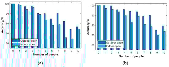
Figure 9.
Experimental results in different environments. (a) shows the true accuracy. (b) shows the accuracy within error ±1.
As depicted in Figure 9a, the true accuracies of the proposed model in both environments (outdoor and indoor open environments) decrease to different degrees with the increasing number of subjects, and the true accuracy declines more slowly in the outdoor open environment compared with the indoor open environment. In the indoor open environment, when the number of people in the ROI region reaches 4, the accuracy decreases to below 90% for the first time. Still, in the outdoor open environment, when the amount of people in the ROI region reaches 6, the accuracy declines to below 90% for the first time. The reason for the above result is that in the indoor open environment, there are walls around, and the rebar and concrete in the walls affect the IR-UWB radar echoes. Thus, the true accuracy in the outdoor open environment is generally better than in the indoor open environment.
Figure 9b presents the accuracies within ±1 error using Equation (24) for two different experimental environments (i.e., outdoor and indoor open environments). As depicted in Figure 9b, in the outdoor open environment, the accuracy within error ±1 achieved an accuracy of 90% in detecting the number of people in the ROI area within 0–6. As an experimental control group, in the indoor open environment, the accuracy within error ±1 reached 90% in detecting the number of people in the ROI area within 0–3, and the accuracy was 80% when the subject target reached 8. Based on the calculation, the test results of 89.37% true accuracy and 92.10% accuracy within error ± 1 on average in an outdoor open environment were obtained, and the experimental results are listed in Table 4. In another indoor open environment, an average of 83.96% in terms of of true accuracy and 86.60% in terms of accuracy within error ± 1 of the test results were achieved. The experimental results are listed in Table 5.
Table 4.
Outdoor open environment.
Table 5.
Indoor open environment.
4.2.2. Confusion Matrix
In this section, we will assess the performance of the 1DCNN-LSTM model proposed for this study using a confusion matrix. A confusion matrix, also known as an error matrix, is a commonly employed tool for visually evaluating the performance of supervised learning algorithms. In two subject environments (including an outdoor open environment and an indoor open environment), the number of subjects is estimated from 0 to 10 using the 1DCNN-LSTM model proposed in this study. The results of the confusion matrix for the outdoor open environment are shown in Figure 10, and the results of the confusion matrix for the indoor open environment are shown in Figure 11.
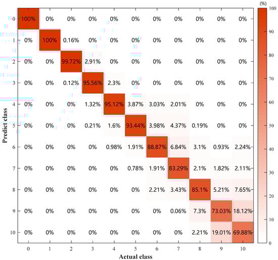
Figure 10.
Confusion matrix for different number of detections in outdoor open environment.

Figure 11.
Confusion matrix of different numbers of detections in the indoor open environment.
Figure 10 presents the confusion matrix of different detection numbers in the outdoor open environment, where the horizontal coordinate represents the practical value of the detection numbers in the ROI region of the practical test environment. The vertical coordinate represents the predicted value of the people counting in the ROI region using the proposed 1DCNN-LSTM model to predict the people counting in the IR-UWB radar signals. First, the results suggested that the prediction accuracy declined with the gradual increase in the subject targets, with the maximum prediction of 0 and 1 as the maximum value of 100% and the minimum prediction of 10 as the minimum value of 69.88%. The reason for this result is that when the number of people in the ROI region gradually increased, a multipath effect was significantly formed, generating considerable multipath signals and thus leading to inaccurate prediction. Second, due to the setting of the experimental environment in this study, we failed to fix the position of the subjects. In other words, the participants were granted to walk around freely in the ROI area. The randomness of the subject targets resulted in some errors in the number of predictions using the 1DCNN-LSTM model proposed in this study. In addition, due to the increase in the number of people, the neighboring feature vectors overlapped, resulting in an increase or decrease in the number of predictions (e.g., the predictions of eight and nine people). Although there was a certain probability of prediction error in the above case, this prediction error was limited to the number of neighboring predictions by calculating the number of predictions. Thus, the accuracy with error ±1/% in the previous section was counted. Lastly, as indicated by the confusion matrix of different detection numbers in the outdoor open environment in Figure 10, although there was a certain false detection rate, the overall tendency was under a high accuracy rate, especially during the detection of five people or less, the detection accuracy rate was as high as 90%. Furthermore, the average accuracy rate was calculated as 89.37% in the outdoor open environment, thus confirming the high accuracy rate of the proposed model in this study.
Figure 11 presents the confusion matrix for different detection numbers in the indoor empty environment, the horizontal coordinate represents the real value of the detection numbers in the ROI region of the practical test environment, and the vertical coordinate represents the prediction value of the number of people obtained using the 1DCNN-LSTM model. Similar to the outdoor empty environment, the prediction accuracy tended to decrease with the increasing number of people in the ROI region, with the maximum being the case of detecting 0 people with 100% detection accuracy and the minimum being the case of detecting 10 people with only 61.53% detection accuracy. As indicated by the comparison of Figure 10 and Figure 11 for the outdoor empty environment, the accuracy of the 1DCNN-LSTM model in the indoor environment was overall lower than that in the outdoor environment. The reason for this result is the presence of walls and ceilings in the indoor open environment, which can also lead to the generation of more multipath signals. As depicted in Figure 11, the 1DCNN-LSTM model proposed in this study was robust due to the low echo SNR generated by IR-UWB radar in indoor environments. However, the proposed model can still have a high accuracy in low SNR environments, and it is only when detecting approximately up to eight people that the model accuracy drops below 80%. Moreover, the average accuracy was calculated as 83.96% in the outdoor open environment, thus proving the high accuracy and robustness of the proposed model in this study.
4.2.3. ROC Curve and CDF
To further validate the performance of the proposed 1DCNN-LSTM model in two experimental environments (outdoor and indoor open environments) excerpted when the subject target was three, the Receiver Operating Characteristic (ROC) curves as well as the Cumulative Distribution Function (CDF), the experimental results were plotted in Figure 12a and Figure 12b, respectively. The ROC curves, indicating the different thresholds that can be applied to the classifier’s output when the classifier’s output is binary (e.g., an instance belongs to a certain class or not), were represented in this subsection for the predicted number of three people.
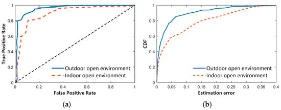
Figure 12.
Performance metrics under different experimental environments. (a) ROC curve. (b) CDF plot.
Figure 12a shows the ROC curves in different experimental environments obtained under the number of targets of three. As indicated by the horizontal coordinate FPR, the proposed 1DCNN-LSTM model was misclassified as a negative case. As indicated by the vertical coordinate TPR, the proposed 1DCNN-LSTM model was correctly categorized and was a positive case. As depicted in Figure 12a, the ROC curve in the outdoor open environment was above the indoor open environment. On the other hand, it can be better understood using another metric, i.e., the total Area under Curve (AUC) area below the ROC curve. As depicted in Figure 12a, the AUC area in the outdoor open environment was larger than that in the indoor open environment, which was calculated as 0.96 in the outdoor open environment and 0.88 in the indoor open environment. Figure 12b presents the CDF plots of the different subjective environments with the number of people of only three by using the proposed 1DCNN-LSTM model, which is the probability density function (CDF). CDF is capable of representing the effect of error accumulation, with the horizontal coordinate representing the recognition error rate and the vertical axis representing the CDF value. Maximum accuracy was achieved in the outdoor open environment, where approximately 92% of the test data achieved an error rate of less than 10%. Minimum accuracy was achieved in the indoor open environment, where approximately 63% of the test data achieved an error rate of less than 10%. Notably, in the outdoor open environment, the cumulative distribution function of the error rate was in the upper part of the indoor open environment, i.e., the closer the curve to the upper left, the better the recognition effect of the classification, and the more accurate the results. In other words, the closer it is to the number of people in the region, the closer it is to the true value of the ROI. In general, the proposed 1DCNN-LSTM model is capable of maintaining a good recognition resolution in both subject environments and conforming to the universal subject environment for detection.
4.2.4. Performance Evaluation of Different Methods
Several existing typical ROI region people counting detection algorithms were compared using ROC curves to further analyze and validate the performance of the proposed model. We trained different algorithms using the same training samples and test sets in an outdoor open environment as well as an indoor open environment. The experimental results are presented in Figure 13a and Figure 13b, respectively.
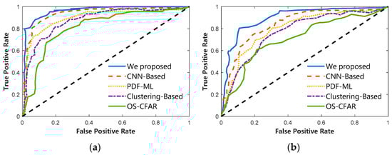
Figure 13.
ROC curves in different experimental environments. (a) Outdoor open environment with the same samples. (b) Indoor open environment with the same samples.
Figure 13a,b present the average ROC curves for the data obtained from five people counting algorithms are plotted for the same training samples and test set in an outdoor open environment and indoor open environment, respectively. The five algorithms include (1) the 1DCNN-LSTM algorithm that we proposed, (2) a CNN-based algorithm, (3) the PDF-ML algorithm, (4) a clustering-based algorithm, and (5) the OS-CFAR algorithm. As depicted in Figure 13a,b, the proposed 1DCNN-LSTM algorithm is highly competitive, i.e., higher accuracy algorithms are effective. We found that the OS-CFAR algorithm has lower accuracy and effectiveness, i.e., the AUC area is minimum. Furthermore, the average accuracy, average recall, and average F1-score of the classification algorithms were calculated. The detailed results of the calculations are listed in Table 6. As depicted in Table 6, the average accuracy of the proposed algorithm in this study reached up to 86.66%, higher than the remaining four comparison algorithms, i.e., the 1DCNN-LSTM algorithm proposed in this study exhibited high accuracy.
Table 6.
Mean accuracy, recall, and F1-score for different algorithms.
5. Discussion
This study aimed at designing algorithms that can effectively differentiate people counting in the ROI region with high accuracy and ease of implementation. For people counting using IR-UWB conventional methods, it is difficult to set the optimal threshold due to using a single threshold, and there exists a problem that people counting cannot be determined at low SNR under the effects of multipath and noise signals. In this study, a 1DCNN-LSTM-based excess kurtosis people counting system was proposed using IR-UWB radar signals. Using actual IR-UWB radar sensors, we validate the algorithm’s performance in two open environments. We found that the greater the subject’s weight, the more reflected signals the radar picks up, which increases the number of pulse frames, which may cause the algorithm to experience an increased counting error rate. In order to control the variable to reduce the variability caused by weight, we selected the same volunteers (as shown in Table 3) as experimental subjects. In this paper, the ROI region, we simulate the actual application scenarios such as shopping malls, halls, outdoor, and other open environments. We set the size of the experimental environment as a 6 m × 6 m open environment. However, even so, when we apply the proposed 1DCNN-LSTM algorithm to the complex environment in the laboratory, we find that it is also effective because we use the running average method to eliminate the static clutter in the background. At the same time, we use the Butterworth filter to improve the SNR of IR-UWB radar signals. Non-static noise signals mainly influence IR-UWB radar signals in complex environments, so it is wise to use smoothing filters to suppress non-static noise signals.
Thus, this study was subjected to the following limitations. In this study, the data were collected only in a stationary scene, the effects exerted by scene migration were ignored, and only an empty environment was considered not a complex experimental scene with more clutter (e.g., computers and obstacles). Accordingly, in subsequent research, the relevant research will be conducted on the following two points. (1) Training via data-enhanced training networks or other datasets is conducted to enhance the scene migration generalization ability of the proposed algorithm. (2) Moreover, relevant experimental studies are conducted for complex experimental scenarios to refine and optimize the algorithm.
6. Conclusions
In this study, a 1DCNN-LSTM-based excess kurtosis people counting system was proposed, using IR-UWB radar signals. The proposed algorithm solved the problem of optimal threshold setting by extracting the human signals to form a feature vector using different thresholds. A feature vector from the respective formed frame was developed by bundling the preprocessed IR-UWB radar signal pulses into frames. The human-induced excess kurtosis was detected using a modified CLEAN algorithm by varying the threshold value. Next, the formed peaks were grouped for subsequent training and validation. The performance of the proposed model for different detection ROIs and different subjects was analyzed, and the experiments were performed in outdoor and indoor open environments. Based on the calculation, the test results of 89.37% true accuracy and 92.10% accuracy within ±1 error on average were obtained in the outdoor open environment. In addition, the average 83.96% true accuracy and 86.60% accuracy within error ±1 were obtained in the indoor open environment. As indicated by the results, the algorithm can apply to scenarios with large detection angles and large detection ranges while exhibiting high stability. Furthermore, the algorithm achieved high accuracy, robustness, and ease of implementation through comparative experiments compared with other people counting detection methods proposed over the past few years. The proposed 1DCNN-LSTM algorithm had an average accuracy of 86.66% for recognizing ROIs. The proposed 1DCNN-LSTM algorithm can be used for IR-UWB radar for sensing the people counting field. The algorithm can be effectively applied to monitor the number of people in a focused area as it is not affected by conditions such as illumination, and at the same time, privacy issues can be effectively avoided.
Author Contributions
J.Z. and X.D. conceived and designed the experiments; J.Z. performed the experiments; J.Z. and X.D. analyzed the data and wrote the paper. J.Z. and Z.H. helped in writing the introduction and the related works and critically revised the paper; Z.H. revised the equations, and critically revised the paper. All authors have read and agreed to the published version of the manuscript.
Funding
This research was funded by the National Natural Science Foundation of China (Grant 62162056), Industrial Support Foundations of Gansu (Grant No. 2021CYZC-06).
Institutional Review Board Statement
Not applicable.
Informed Consent Statement
Informed consent was obtained from all subjects involved in the study. Written informed consent has been obtained from the subjects to publish this paper.
Data Availability Statement
Data are contained within the article.
Acknowledgments
The authors would like to thank the reviewers for their thorough reviews and helpful suggestions.
Conflicts of Interest
The authors declare no conflict of interest.
References
- Zhang, J.; Tao, D. Empowering things with intelligence: A survey of the progress, challenges, and opportunities in artificial intelligence of things. IEEE Internet Things J. 2020, 8, 7789–7817. [Google Scholar] [CrossRef]
- Guo, J.; Gu, X.; Liu, Z.; Ji, M.; Wang, J.; Yin, X.; Xu, P. CM-NET: Cross-Modal Learning Network for CSI-Based Indoor People Counting in Internet of Things. Electronics 2022, 11, 4113. [Google Scholar] [CrossRef]
- Sam, D.B.; Peri, S.V.; Sundararaman, M.N.; Kamath, A.; Babu, R.V. Locate, size, and count: Accurately resolving people in dense crowds via detection. IEEE Trans. Pattern Anal. Mach. Intell. 2020, 43, 2739–2751. [Google Scholar]
- Sindagi, V.A.; Yasarla, R.; Patel, V.M. Jhu-crowd++: Large-scale crowd counting dataset and a benchmark method. IEEE Trans. Pattern Anal. Mach. Intell. 2020, 44, 2594–2609. [Google Scholar] [CrossRef]
- Wu, D.; Fan, Z.; Yi, S. Crowd Counting based on Multi-level Multi-scale Feature. Appl. Intell. 2023, 1–11. [Google Scholar] [CrossRef]
- Liu, S.; Zhao, Y.; Chen, B. WiCount: A deep learning approach for crowd counting using WiFi signals. In Proceedings of the 2017 IEEE International Symposium on Parallel and Distributed Processing with Applications and 2017 IEEE International Conference on Ubiquitous Computing and Communications (ISPA/IUCC), IEEE, Guangzhou, China, 12–15 December 2017; pp. 967–974. [Google Scholar]
- Yuan, Y.; Zhao, J.; Qiu, C.; Xi, W. Estimating crowd density in an RF-based dynamic environment. IEEE Sens. J. 2013, 13, 3837–3845. [Google Scholar] [CrossRef]
- Ding, H.; Han, J.; Liu, A.X.; Xi, W.; Zhao, J.; Yang, P.; Jiang, Z. Counting human objects using backscattered radio frequency signals. IEEE Trans. Mob. Comput. 2018, 18, 1054–1067. [Google Scholar] [CrossRef]
- Xu, C.; Firner, B.; Moore, R.S.; Zhang, Y.; Trappe, W.; Howard, R.; Zhang, F.; An, N. SCPL: Indoor device-free multi-subject counting and localization using radio signal strength. In Proceedings of the 12th International Conference on Information Processing in Sensor Networks, Philadelphia, PA, USA, 8–11 April 2013; pp. 79–90. [Google Scholar]
- Jiang, H.; Chen, S.; Xiao, Z.; Hu, J.; Liu, J.; Dustdar, S. Pa-Count: Passenger Counting in Vehicles Using Wi-Fi Signals. IEEE Trans. Mob. Comput. 2023, 1–14. [Google Scholar] [CrossRef]
- Hagenaars, E.; Pandharipande, A.; Murthy, A.; Leus, G. Single-pixel thermopile infrared sensing for people counting. IEEE Sens. J. 2020, 21, 4866–4873. [Google Scholar] [CrossRef]
- Samuel, M.; Samuel-soma, M.A.; Moveh, F.F. AI Driven Thermal People Counting for Smart Window Facade Using Portable Low-Cost Miniature Thermal Imaging Sensors. Preprints 2020, 45, 2020010067. [Google Scholar] [CrossRef][Green Version]
- Federal Communications Commission. In the Matter of Revision of Part 15 of the Commission’s Rules Regarding Ultra-WIDEBAND Transmission Systems; First Report and Order, ET Docket 98-153; Federal Communications Commission: Washington, DC, USA, 2002. [Google Scholar]
- Choi, S.H.; Yoon, H. Convolutional Neural Networks for the Real-Time Monitoring of Vital Signs Based on Impulse Radio Ultrawide-Band Radar during Sleep. Sensors 2023, 23, 3116. [Google Scholar] [CrossRef] [PubMed]
- Chiasson, D.; Lin, Y.; Kok, M.; Shull, P. Asynchronous Hyperbolic UWB Source-Localization and Self-Localization for Indoor Tracking and Navigation. IEEE Internet Things J. 2023, 10, 11655–11668. [Google Scholar] [CrossRef]
- Santoro, L.; Nardello, M.; Brunelli, D.; Fontanelli, D. UWB-based Indoor Positioning System with Infinite Scalability. IEEE Trans. Instrum. Meas. 2023, 72, 1005711. [Google Scholar] [CrossRef]
- Andersen, N.; Granhaug, K.; Michaelsen, J.A.; Bagga, S.; Hjortland, H.A.; Knutsen, M.R.; Lande, T.S.; Wisland, D.T. A 118-mW 23.3-GS/s dual-band 7.3-GHz and 8.7-GHz impulse-based direct RF sampling radar SoC in 55-nm CMOS. In Proceedings of the 2017 IEEE International Solid-State Circuits Conference (ISSCC), IEEE, San Francisco, CA, USA, 5–9 February 2017; pp. 138–139. [Google Scholar]
- Ren, L.; Yarovoy, A.; Fioranelli, F. Grouped People Counting Using mm-wave FMCW MIMO Radar. IEEE Internet Things J. 2023. [Google Scholar] [CrossRef]
- Choi, J.W.; Cho, S.H.; Kim, Y.S.; Kim, N.J.; Kwon, S.S.; Shim, J.S. A counting sensor for inbound and outbound people using IR-UWB radar sensors. In Proceedings of the 2016 IEEE Sensors Applications Symposium (SAS), IEEE, Catania, Italy, 20–22 April 2016; pp. 1–5. [Google Scholar]
- Choi, J.W.; Quan, X.; Cho, S.H. Bi-directional passing people counting system based on IR-UWB radar sensors. IEEE Internet Things J. 2017, 5, 512–522. [Google Scholar] [CrossRef]
- Choi, J.W.; Nam, S.S.; Cho, S.H. Multi-human detection algorithm based on an impulse radio ultra-wideband radar system. IEEE Access 2016, 4, 10300–10309. [Google Scholar] [CrossRef]
- Bartoletti, S.; Conti, A.; Win, M.Z. Device-free counting via wideband signals. IEEE J. Sel. Areas Commun. 2017, 35, 1163–1174. [Google Scholar] [CrossRef]
- Choi, J.W.; Yim, D.H.; Cho, S.H. People counting based on an IR-UWB radar sensor. IEEE Sens. J. 2017, 17, 5717–5727. [Google Scholar] [CrossRef]
- Choi, J.W.; Kim, J.H.; Cho, S.H. A counting algorithm for multiple objects using an IR-UWB radar system. In Proceedings of the 2012 3rd IEEE International Conference on Network Infrastructure and Digital Content, IEEE, Beijing, China, 21–23 September 2012; pp. 591–595. [Google Scholar]
- Choi, J.W.; Cho, S.H. A crowdedness measurement algorithm using an IR-UWB radar sensor. In Future Communication, Information and Computer Science: Proceedings of the 2014 International Conference on Future Communication, Information and Computer Science (FCICS 2014), Beijing, China, 22–23 May 2014; CRC Press: Boca Raton, FL, USA; p. 119.
- Wei, K.; Fang, S.; Tao, J. Enhanced Near-Field Interference Suppression Scheme for the Non-Cooperative Underwater Acoustic Pulse Detection of the Towed Linear Array. J. Mar. Sci. Eng. 2022, 10, 250. [Google Scholar] [CrossRef]
- Perrotta, A.M.; Maffucci, A.; Ventre, S.; Tamburrino, A. Efficient Near-Field Analysis of the Electromagnetic Scattering Based on the Dirichlet-to-Neumann Map. Appl. Sci. 2019, 9, 4179. [Google Scholar] [CrossRef]
- Tan, F.; Bao, C.; Zhou, J. Effective Dereverberation with a Lower Complexity at Presence of the Noise. Appl. Sci. 2022, 12, 11819. [Google Scholar] [CrossRef]
- Goldhahn, R.; Hickman, G.; Krolik, J. Waveguide invariant broadband target detection and reverberation estimation. J. Acoust. Soc. Am. 2008, 124, 2841–2851. [Google Scholar] [CrossRef]
- Yang, X.; Yin, W.; Li, L.; Zhang, L. Dense people counting using IR-UWB radar with a hybrid feature extraction method. IEEE Geosci. Remote Sens. Lett. 2018, 16, 30–34. [Google Scholar] [CrossRef]
- Yin, W.; Yang, X.; Zhang, L.; Oki, E. ECG monitoring system integrated with IR-UWB radar based on CNN. IEEE Access 2016, 4, 6344–6351. [Google Scholar] [CrossRef]
- Deng, L.; Zhou, Q.; Wang, S.; Górriz, J.M.; Zhang, Y. Deep learning in crowd counting: A survey. CAAI Trans. Intell. Technol. 2023, 1–35. [Google Scholar] [CrossRef]
- Alhussein, M.; Aurangzeb, K.; Haider, S.I. Hybrid CNN-LSTM model for short-term individual household load forecasting. IEEE Access 2020, 8, 180544–180557. [Google Scholar] [CrossRef]
- Choi, S.H.; Kwon, H.B.; Jin, H.W.; Yoon, H.; Lee, M.H.; Lee, Y.J.; Park, K.S. Long short-term memory networks for unconstrained sleep stage classification using polyvinylidene fluoride film sensor. IEEE J. Biomed. Health Inform. 2020, 24, 3606–3615. [Google Scholar] [CrossRef]
- Lee, D.; Kwon, H.; Son, D.; Eom, H.; Park, C.; Lim, Y.; Seo, C.; Park, K. Beat-to-beat continuous blood pressure estimation using bidirectional long short-term memory network. Sensors 2020, 21, 96. [Google Scholar] [CrossRef] [PubMed]
- Bao, R.; Yang, Z. CNN-based regional people counting algorithm exploiting multi-scale range-time maps with an IR-UWB radar. IEEE Sens. J. 2021, 21, 13704–13713. [Google Scholar] [CrossRef]
- Xu, Y.; Dai, S.; Wu, S.; Chen, J.; Fang, G. Vital sign detection method based on multiple higher order cumulant for ultrawideband radar. IEEE Trans. Geosci. Remote Sens. 2011, 50, 1254–1265. [Google Scholar] [CrossRef]
- Rawat, W.; Wang, Z. Deep convolutional neural networks for image classification: A comprehensive review. Neural Comput. 2017, 29, 2352–2449. [Google Scholar] [CrossRef] [PubMed]
- Shafiq, M.; Gu, Z. Deep residual learning for image recognition: A survey. Appl. Sci. 2022, 12, 8972. [Google Scholar] [CrossRef]
- Szegedy, C.; Liu, W.; Jia, Y.; Sermanet, P.; Reed, S.; Anguelov, D.; Erhan, D.; Vanhoucke, V.; Rabinovich, A. Going deeper with convolutions. In Proceedings of the IEEE Conference on Computer Vision and Pattern Recognition, Boston, MA, USA, 7–12 June 2015; pp. 1–9. [Google Scholar]
- Zhu, J.; Chen, H.; Ye, W. A hybrid CNN–LSTM network for the classification of human activities based on micro-Doppler radar. IEEE Access 2020, 8, 24713–24720. [Google Scholar] [CrossRef]
- Kingma, D.P.; Ba, J. Adam: A method for stochastic optimization. arXiv 2014, arXiv:1412.6980. [Google Scholar]
- He, K.; Zhang, X.; Ren, S.; Sun, J. Delving deep into rectifiers: Surpassing human-level performance on imagenet classification. In Proceedings of the IEEE International Conference on Computer Vision, Santiago, Chile, 7–13 December 2015; pp. 1026–1034. [Google Scholar]
- Moolayil, J. An introduction to deep learning and keras. In Learn Keras for Deep Neural Networks: A Fast-Track Approach to Modern Deep Learning with Python; Apress: Berkeley, CA, USA, 2019; pp. 1–16. [Google Scholar]
- Abadi, M.; Barham, P.; Chen, J.; Chen, Z.; Davis, A.; Dean, J.; Devin, M.; Ghemawat, S.; Goodfellow, I.; Zheng, X.; et al. {TensorFlow}: A system for {Large-Scale} machine learning. In Proceedings of the 12th USENIX Symposium on Operating Systems Design and Implementation (OSDI 16), Savannah, GA, USA, 2–4 November 2016; pp. 265–283. [Google Scholar]
- Ioffe, S.; Szegedy, C. Batch normalization: Accelerating deep network training by reducing internal covariate shift. In Proceedings of the International Conference on Machine Learning, Lille, France, 6–11 July 2015; pp. 448–456. [Google Scholar]
- Goodfellow, I.; Bengio, Y.; Courville, A. Deep Learning; MIT Press: Cambridge, MA, USA, 2016. [Google Scholar]
- Yu, Y.; Si, X.; Hu, C.; Zhang, J. A review of recurrent neural networks: LSTM cells and network architectures. Neural Comput. 2019, 31, 1235–1270. [Google Scholar] [CrossRef] [PubMed]
- Van der Walt, C.M.; Barnard, E. Data characteristics that determine classifier performance. SAIEE Afr. Res. J. 2007, 98, 87–93. [Google Scholar] [CrossRef]
- Gandhi, P.P.; Kassam, S.A. Analysis of CFAR processors in nonhomogeneous background. IEEE Trans. Aerosp. Electron. Syst. 1988, 24, 427–445. [Google Scholar] [CrossRef]
Disclaimer/Publisher’s Note: The statements, opinions and data contained in all publications are solely those of the individual author(s) and contributor(s) and not of MDPI and/or the editor(s). MDPI and/or the editor(s) disclaim responsibility for any injury to people or property resulting from any ideas, methods, instructions or products referred to in the content. |
© 2023 by the authors. Licensee MDPI, Basel, Switzerland. This article is an open access article distributed under the terms and conditions of the Creative Commons Attribution (CC BY) license (https://creativecommons.org/licenses/by/4.0/).