An Image Enhancement Method for Side-Scan Sonar Images Based on Multi-Stage Repairing Image Fusion

Abstract

The noise interference of side-scan sonar images is stronger than that of optical images, and the gray level is uneven. To solve this problem, we propose a side-scan sonar image enhancement method based on multi-stage repairing image fusion. Firstly, to remove the environmental noise in the sonar image, we perform adaptive Gaussian smoothing on the original image and the weighted average grayscale image. Then, the smoothed images are all processed through multi-stage image repair. The multi-stage repair network consists of three stages. The first two stages consist of a novel encoder–decoder architecture to extract multi-scale contextual features, and the third stage uses a network based on the resolution of the original inputs to generate spatially accurate outputs. Each phase is not a simple stack. Between each phase, the supervised attention module (SAM) improves the repair results of the previous phase and passes them to the next phase. At the same time, the multi-scale cross-stage feature fusion mechanism (MCFF) is used to complete the information lost in the repair process. Finally, to correct the gray level, we propose a pixel-weighted fusion method based on the unsupervised color correction method (UCM), which performs weighted pixel fusion between the RGB image processed by the UCM algorithm and the gray-level image. Compared with the algorithm with the SOTA methods on datasets, our method shows that the peak signal-to-noise ratio (PSNR) is increased by 26.58%, the structural similarity (SSIM) is increased by 0.68%, and the mean square error (MSE) is decreased by 65.02% on average. In addition, the processed image is balanced in terms of image chromaticity, image contrast, and saturation, and the grayscale is balanced to match human visual perception.

1. Introduction

Side-scan sonar has the advantages of high resolution, low cost, simple operation, and continuous acquisition of seabed images. Therefore, by using side-scan sonar to scan the seabed, seabed scenes and topographic information can be obtained. Application scenarios include offshore oil drilling, channel dredging, submarine pipeline detection, submarine structure detection, marine environment detection, marine archaeology, and detection and positioning of large submarine targets.

The basic working principle of side-scan sonar is similar to that of side-looking radar. A linear array of transducers is installed on the left and right sides of the side-scan sonar. With the continuous movement of the underwater sonar carrier, the sonar array continuously transmits and receives processing in the advancing process, and records are arranged line by line, displaying the return data of each transmission line by line on the display [1]. Side-scan sonar image is a gray image without color information. The size of the pixel grayscale depends on the strength of the reflected sound waves from the underwater material. The noise interference of the side-scan sonar image is much stronger than that of the general optical image, which mainly falls into three categories: ambient noise with Gaussian distribution, reverberation noise, and white noise [2]. Due to the interference of the underwater environment, the acquired original side-scan sonar image has many problems such as noise interference, low image contrast, and weak feature information, which affect the matching, stitching, and target recognition of the side-scan sonar image; therefore, before the next processing of the side-scan sonar, denoising is an important step [3,4].

Grabek and Cyganek proposed a tensor-based speckle noise reduction method for side-scan sonar images [5]. Kim et al. proposed an image registration and stitching fusion algorithm for underwater sonar image sequences with high noise, uneven illumination, and low frame rate [6]. In addition, the gray level distribution of the gray map image directly restored by the acoustic signal is generally narrower. So, it is necessary to carry out histogram balancing and grayscale correction processing. Ye et al. proposed a simple and effective gray correction method for sonar side-scan images based on Retinex [1]. The image processing algorithm based on Retinex theory is a commonly used optical image defogging and low-illumination image enhancement algorithm. Burguera et al. analyzed the side-scan sonar imaging model to complete gray correction [7]. Shi et al. proposed an improved dark channel theory to enhance each area of the image, aiming at the problems such as uneven background gray distribution and blurred boundary details in underwater images acquired by sonar [8].

At present, the research on image preprocessing of side-scan sonar has problems of strong pertinence and single function. To meet the demand for both denoising and gray balance, we propose a side-scan sonar image enhancement method based on multi-stage repairing image fusion. In addition, added a list of abbreviations, and additionally decipher each of them the first time they appear.

2. Related Work

2.1. Traditional Grayscale Correction Method

The common gray correction methods of side-scan sonar images include histogram equalization, CLAHE, gamma correction, and RGHS.

Histogram equalization (HE) improves the uniformity of the gray distribution of side-scan sonar images by adjusting the gray distribution of the whole image [9]. The essence of histogram equalization involves enlarging the gray level difference of the image, and the overall contrast of the equalized image is improved. Despite its excellent performance in enhancing the contrast of a given image, histogram equalization tends to increase image noise. Moreover, the weak edges of the image are blurred due to the merging of some gray levels, resulting in excessive enhancement of the regions with large histogram peaks, which is not conducive to processing side-scan sonar images.

The difference between contrast-limited adaptive histogram equalization (CLAHE) and ordinary adaptive histogram equalization is contrast clipping [10]. The contrast of each pixel neighborhood must be limited to obtain the corresponding transformation function. CLAHE can enhance the contrast of the image, make the image clearer, and also avoid the excessive enhancement and noise generation caused by global histogram equalization. The disadvantage is that the image needs to be processed in blocks, which will increase the amount of computation and storage space.

Gamma correction can detect the dark part and light part of the image signal by artificial nonlinear mapping and increase the ratio of the two parts to improve the image contrast effect. The algorithm consists of three parts: normalization, nonlinear mapping, and anti-normalization. Although gamma correction improves the overall contrast of an image, it does not enhance the edges and textures [11]. Therefore, only using gamma correction to process the feature information of a side-scan sonar image is still not obvious. The function of this algorithm is single and limited.

Relative global histogram stretching (RGHS) has been proposed in RGB and CIE-Lab color models [12]. According to the distribution characteristics of RGB channels and the selective attenuation of underwater light propagation, adaptive histogram stretching is used in the RGB color model based on the preprocessed image of the gray world theory. Finally, brightness L and color components a and b in CIE-Lab color space are optimized as linear- and curve-adaptive stretching operations, respectively. RGHS avoids blind enhancement of underwater image features, improves the visual effect of the image, and retains the available information of the image, and the visual effect after processing is indeed good. However, this method is time-consuming, and it takes 30 s to process a 3840 × 2160 image.

All the above algorithms increase the contrast of the image in a certain way, but the effect of the single use of the traditional gray correction algorithm is limited. Therefore, it can be used in combination with image-denoising algorithms to achieve side-scan sonar images with strong feature information, less noise, and gray balance.

2.2. Traditional Image Denoising Methods

Median filtering involves replacing the value of each pixel with the median of its neighboring pixels [13]. This helps to smooth the image and remove speckle noise, but it causes edge blurring to some extent.

Wavelet transform decomposes a signal into different frequency bands [14]. After decomposition, it can remove high-frequency noise while retaining the useful signal. It is very effective in certain cases when the noise frequency range is known and the signal and noise frequency bands are separated from each other, but its denoising effect is poor for white noise which widely exists in practical applications. White noise is also the main noise interference in side-scan sonar images.

The BM3D (block-matching 3D) block-matching algorithm is a good image denoising algorithm [15]. Firstly, BM3D combines the characteristics of non-local self-similarity and transform denoising in the frequency domain. Based on the sparsity of the image in the transform domain, the sparsity is enhanced by stacking similar 2D image patches into 3D groups. Secondly, similar to the NLM non-local means denoising method, BM3D uses non-local self-similarity and proposes a collaborative filtering method. Collaborative filtering is a general term for the grouping and filtering process, which is divided into four steps: searching for similar blocks and grouping them; linear transformation of 3D blocks; shrinkage of transform coefficients; the inverse transform of the 3D block. By matching with adjacent image blocks, several similar blocks are integrated into a three-dimensional matrix, and the filtering process is carried out in three-dimensional space. Then the results are inverse-transformed and fused to two-dimensional to form the denoised image. The denoising effect of this algorithm is remarkable, and the highest peak signal-to-noise ratio can be obtained, but the time complexity is relatively high, so the processing speed is slow.

Bilateral filtering is a compromise process that combines the spatial proximity of images and the similarity of pixel values [16]. Both spatial information and gray similarity are considered to achieve the purpose of edge-preserving and noise extraction. Bilateral filtering is simple, non-iterative, and local and can preserve edges. Wiener filtering or Gaussian filtering is usually used for denoising, but the images will have obvious blurred edges. The protection effect on high-frequency details is not obvious. Bilateral filtering has one more Gaussian covariance than Gaussian filtering, which is based on the Gaussian filtering function of spatial distribution; so, near the edge, the pixels far away will not affect the pixel value of the edge too much, so that the edge pixel value is guaranteed to be preserved [17,18]. Due to saving too much high-frequency information, bilateral filtering cannot clean out the high-frequency noise in the color image and can only filter the low-frequency information well. Moreover, there are many parameters in bilateral filtering, and how to select the appropriate parameter values is also a challenge.

3. Proposed Method

This section mainly illustrates the details of our proposed method. We first present the general structure of the method. Then, adaptive Gaussian filtering is introduced in Section 3.2. Next, in Section 3.3, the new encoder–decoder architecture, which includes the convolutional block attention module (CBAM), the adaptive receptive field mechanism (ARFM), MCFF, and SAM, is introduced along with a description of the loss function. Finally, the pixel-weighted image fusion method based on UCM is proposed in Section 3.4.

The main contributions of this study can be summarized as follows:

• Based on careful consideration of sonar target region features, a novel encoder–decoder CNN architecture is proposed, which can effectively extract features and preserve the original resolution.
• The new loss function is designed to optimize the multi-stage progressive repair network end to end.
• A new improved UCM pixel-weighted fusion grayscale correction method is proposed.

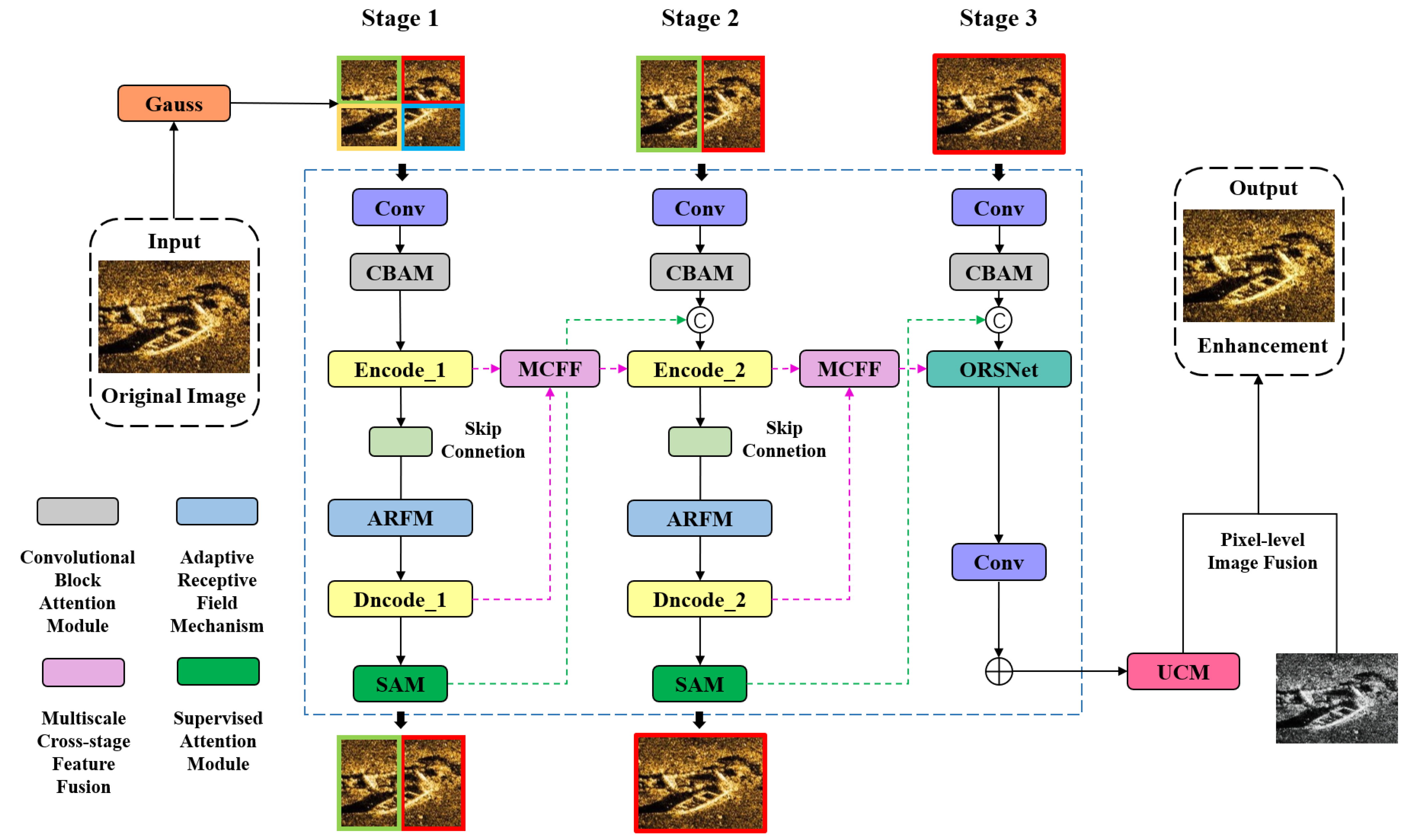
3.1. Overall Architecture

The overall structure of the proposed side-scan sonar image enhancement algorithm based on multi-stage repairing image fusion is shown in Figure 1.

Firstly, in order to remove the environmental noise in the sonar image, we perform adaptive Gaussian smoothing to the original image and to the weighted average grayscale image, and so the Gaussian noise is removed before the images are processed through the progressive image repairing procedure. Then, the smoothed images are all processed through multi-stage progressive image repairing. The multi-stage repairing network consists of three stages. The first two stages are composed of a novel encoder–decoder architecture to extract multi-scale contextual features, and the last stage employs a network based on the original input resolution to generate a spatially accurate output. Each stage is not simply stacked. Between each stage, the repair results of the previous stage are improved by SAM and passed to the next stage. At the same time, MCFF is used to fuse the feature information of the encoder–decoder in the first stage into the encoder in the second stage to complete the information lost in the first stage repair process. The feature information of the encoder–decoder in the second stage is fused into ORSNet in the third stage. Finally, in order to correct the grayscale, we propose a pixel-weighted fusion method based on UCM, which performs weighted pixel fusion between the RGB image processed by UCM and the grayscale image.

3.2. The Adaptive Gaussian Filtering Smoothing Processing

The Gaussian filter algorithm can effectively remove the noise in the image. At the same time as removing the noise, the detailed information in the image will be lost, and the image clarity will be insufficient, resulting in serious image distortion. Due to the shortcomings of the above Gaussian filtering algorithm, as well as the speckle noise of the side-scan sonar image, we propose an improved adaptive Gaussian filtering, which can realize denoising and guarantee image quality. The standard deviation σ of the two-dimensional Gaussian filtering function is improved. This parameter is generally set artificially, which will cause image detail loss and large differences.

When the surface of the medium is not uniform or has special microstructure characteristics, the scattering phenomenon will occur and form a series of coherent waves, which interfere with each other to form speckle noise. Since the scatterers in the resolution unit are randomly distributed, their backscattered energy is also random. Therefore, this echo signal has certain statistical properties. The number of scatterers per unit resolution cell is called the scattering number density. In the ideal case, each resolution cell contains a large number of points scatterers, none of which produces strong reflection signals by itself; in the unit range, the scattering signals of these scatterers are the same, and the speckle follows the Rayleigh distribution. Local feature matching is comparing and calculating the similarity between the local region of the image and the standard noise region by using the characteristics of the standard noise region as the measurement standard, so as to obtain a judgment factor to distinguish the noise region from the region with rich detail information. The higher the matching similarity, the higher the matching degree between the region and the noise region, and a higher degree of smoothing filtering can be applied to the region. The lower the similarity, the lower the matching degree between the region and the speckle noise region, and a lower degree of smoothing filtering can be applied to the region. We can define the similarity as a user-controlled function and implement it as follows:

$$S_{ij}=\frac{1}{1+|v(X_{ij})-v(X_{ref}){|}^2},$$

(1)

$$v(X_{ij})=\frac{{\sigma }^2(X_{ij})}{\mu (X_{ij})},$$

(2)

where $X_{ref}$ is the selected reference blob region, $X_{ij}$ is a local region centered at the pixel $(i,j)$, $v(X_{ref})$ is the variance of the reference region, and $v(X_{ij})$ is the variance of the processing region. The degree of noise blob formation is expressed by the variance and mean ratio ${\sigma }^2/\mu$.

The width of the Gaussian filter can be represented by the standard deviation $\sigma$, which determines how smooth the Gaussian filter is to the image. Therefore, as long as the width parameter of the filter is related to the local region characteristics of the image, the Gaussian filter can filter the image adaptively. The Gaussian filter standard deviation $\sigma$ is calculated by the similarity $S_{ij}$ between the local image region and the reference noise region. The similarity $S_{ij}$ of different regions in the image compared to the reference region is different, so the corresponding standard deviation σ of each region is different. This indicates that the filtering strength of the Gaussian filter is different in different regions of the image. This way, the Gaussian filter can be used to adaptively filter the image. It is ensured that the Gaussian filter can smooth the blob region and the feature region differently. After many experiments, we express the Gaussian standard deviation σ as a quadratic function of region similarity, which is Equation (3), and the image processing effect is the best.

$${\sigma }_{\mathrm{ij}}=2S_{ij}{}^{{}^2}+5.6S_{ij}+1.1,$$

(3)

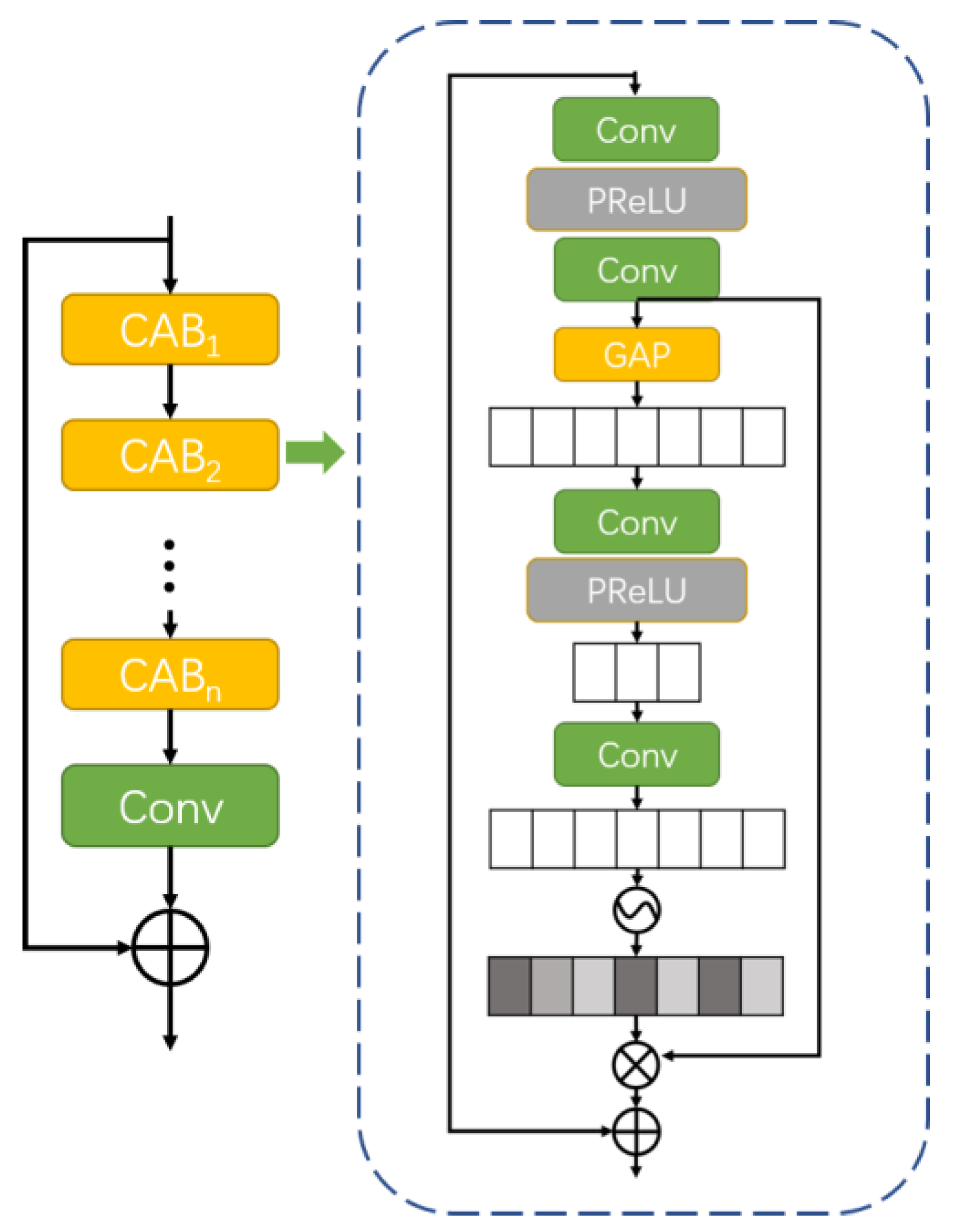
3.3. Multi-Stage Repair Network

The multi-stage repair network consists of three stages. The first two stages consist of a new encoder–decoder architecture to extract multi-scale contextual features. The final stage employs a network based on the original input resolution to generate a spatially accurate output where the new encoder–decoder architecture first extracts a feature at each scale by CBAM, and skip connections are also connected through CBAM. Then, ARFM is used to extract and fuse the interactive feature information, and the decoder uses upsampling and deconvolution to restore the spatial resolution of the feature map. Each stage is not simply stacked. Between each stage, SAM improves the repair results of the previous stage and passes them to the next stage. At the same time, MCFF is used to fuse the feature information of the encoder–decoder of the first stage into the encoder of the second stage to complete the information lost in the repair process of the first stage, and the feature information of the encoder–decoder of the second stage is fused into ORSNet.

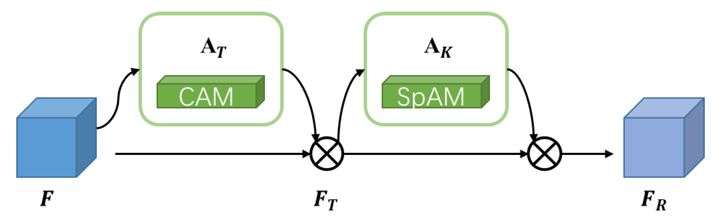
3.3.1. Convolutional Block Attention Module

CBAM is a two-dimensional attention mechanism module, which combines the channel attention module (CAM) and the spatial attention module (SpAM), as shown in Figure 2. The traditional attention mechanism based on the convolutional neural network pays more attention to the analysis of the channel domain and is limited to considering the relationship between the channels of the feature map. Starting from the two scopes of channel and space, CBAM introduces the two analysis dimensions of spatial attention and channel attention to realize the sequential attention structure from channel to space. Spatial attention makes the neural network pay more attention to the pixel regions that play a decisive role in the classification of the image and ignore the irrelevant regions. Channel attention is used to deal with the allocation relationship of the feature map channels. There is a small number of convolution structures and a small number of pooling layers and feature fusion operations in the CBAM module. This structure avoids a large number of calculations caused by convolution multiplication and reduces the complexity and calculation amount. The CBAM module highlights the main features and suppresses irrelevant features, so that the network pays more attention to the content information and location information of the target that needs to be detected and improves the detection accuracy of the network.

When using CBAM, a feature map F is inputted first, the number of channels is C, and the width and height of each channel feature map are W and H, respectively. CBAM uses the channel attention module to convert the input feature map F into a one-dimensional channel attention map A_T, and then the input feature maps F and A_T are multiplied at the pixel level to obtain the channel salient feature map F_T. The calculation formula is as follows:

$$F_T=A_T(F)\otimes F,$$

(4)

Then, we use the spatial attention module to convert F_T into a two-dimensional spatial attention map A_K, and finally, the output feature map F_R is obtained through pixel-wise multiplication of F_T and A_K. The formula is as follows:

$$F_R=A_K(F_T)\otimes F_T,$$

(5)

where $\otimes$ stands for pixel-wise multiplication; the above process is shown in the figure below.

3.3.2. Adaptive Receptive Field Mechanism

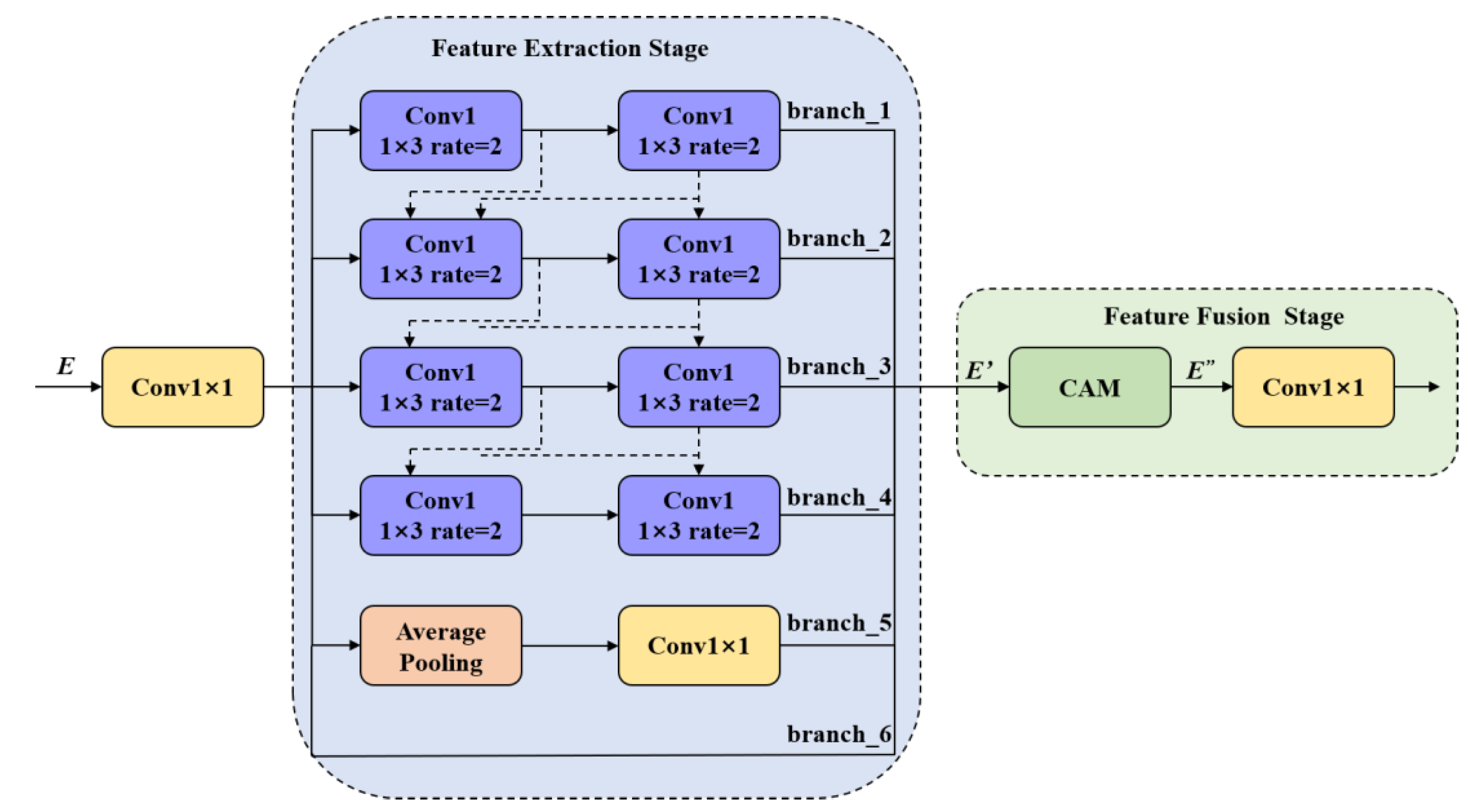
In order to extract the target features of different shapes in side-scan sonar images more accurately, the adaptive perceptual field mechanism block (ARMF) is introduced into the new encoder–decoder CNN architecture. And the convolutional layer feature maps are further processed to extract the features of different perceptual fields. The structure of ARFM is shown in Figure 3, including the feature extraction stage (FES) and the feature fusion stage (FFS). In FES, asymmetric convolution is used to extract receptive field features at different scales. In FFS, CAM is used to channel weight the feature maps of different receptive fields, so that the model pays more attention to the receptive field features with high-target shape fitting.

Feature extraction stage. The FES uses a parallel branch structure to extract features. The first four branches use asymmetric convolutions that skip connections between branches and obtain features of different shapes and sizes. Specifically, 1 × 1 convolution is used to reduce the number of channels of the input feature map E and feed it to different branches. Asymmetric convolution kernels are used in branches 1~4 with dilation rates of 2, 3, 4, and 5, respectively. The original expansion rate k and the size of the 3 × 3 convolutional layer are the features extracted in the square region. However, asymmetric convolution divides the original convolution into two steps, first using a 1 × 3 convolution kernel to extract the lateral region features, and then using a 3 × 1 convolution kernel to extract the vertical region features. Since 1 × 3 and 3 × 1 convolution kernels can expand the receptive field horizontally and vertically, in Figure 3, ARMF uses skip connections to transmit the convolutional layer feature maps of different branches, so that each connection path corresponds to a rectangular receptive field with different proportions. When 1 × 3 and 3 × 1 convolutions with the same dilation rate appear in pairs on the connection path, the generated perceptual field is square. Otherwise, a single 1 × 3 or 3 × 1 convolution appears on the connected path to obtain perceptual fields with different aspect ratios. The aspect ratio of the sensing field for each connected path is calculated as follows.

Feature-mapping perceptual field computation. The feature map E comes from the convolutional layer with a perceptual field shape of a square and an edge length l_z calculated as

$$l_z=l_{z-1}+(f_z-1)\times {\displaystyle \prod _{i=1}^{z-1}{s}_i},$$

(6)

where l_z and l_z−1 represent the edge length of the perceptual field corresponding to layer zth and layer (z − 1)th, respectively; f_z represents the convolution kernel and pooling size at layer zth; s_i represents the convolution kernel and pooling stride of layer zth; the size of the sensing field obtained by layer zth is l_z × l_z.

Single-path sensing field computation. Suppose that the connected path contains m number of 3 × 1 asymmetric convolutions and n number of 1 × 3 asymmetric convolutions, and k is the number of convolutional layers of the connected path, where k = m + n. The height h_m and width w_n of the sensing field of each connected path are calculated as

$$h_m=h_{m-1}+(2\times d_m)\times {\displaystyle \prod _{i=1}^{m-1}{s}_i},$$

(7)

$$w_n=w_{n-1}+(2\times d_n)\times {\displaystyle \prod _{i=1}^{n-1}{s}_i},$$

(8)

where h_m−1 represents the 3 × 1 convolution height corresponding to the perceptual field at layer (m − 1)th in the connected path; d_m represents the expansion rate of the mth layer in the 3 × 1 convolution in the connected path; s_i represents the convolution stride of the ith layer; w_n−1 represents the width of the 1 × 3 convolutional sensing field at layer (n − 1)th of the connected path; d_n represents the expansion rate of the nth layer in the connected path in the 3 × 1 convolution; the perceptual field size of the 3 × 1 and 1 × 3 convolutional layers in the connected path is h_m × w_n. Even though different perceptual field features can be extracted in the first four branches of ARMF, since the input feature map E contains a large amount of detailed information, the fifth branch uses the average pooling layer to extract semantic information within different regions, and the sixth branch transmits the feature information to FFS.

Feature fusion stage. To enable the model to adaptively enhance the receptive field and match the target size, we use CAM in FFS to calculate the association information between features of different receptive fields. The receptive field that matches the target shape can obtain more semantic information of the image, to play the role of adaptive receptive field.

3.3.3. Multiscale Cross-Stage Feature Fusion

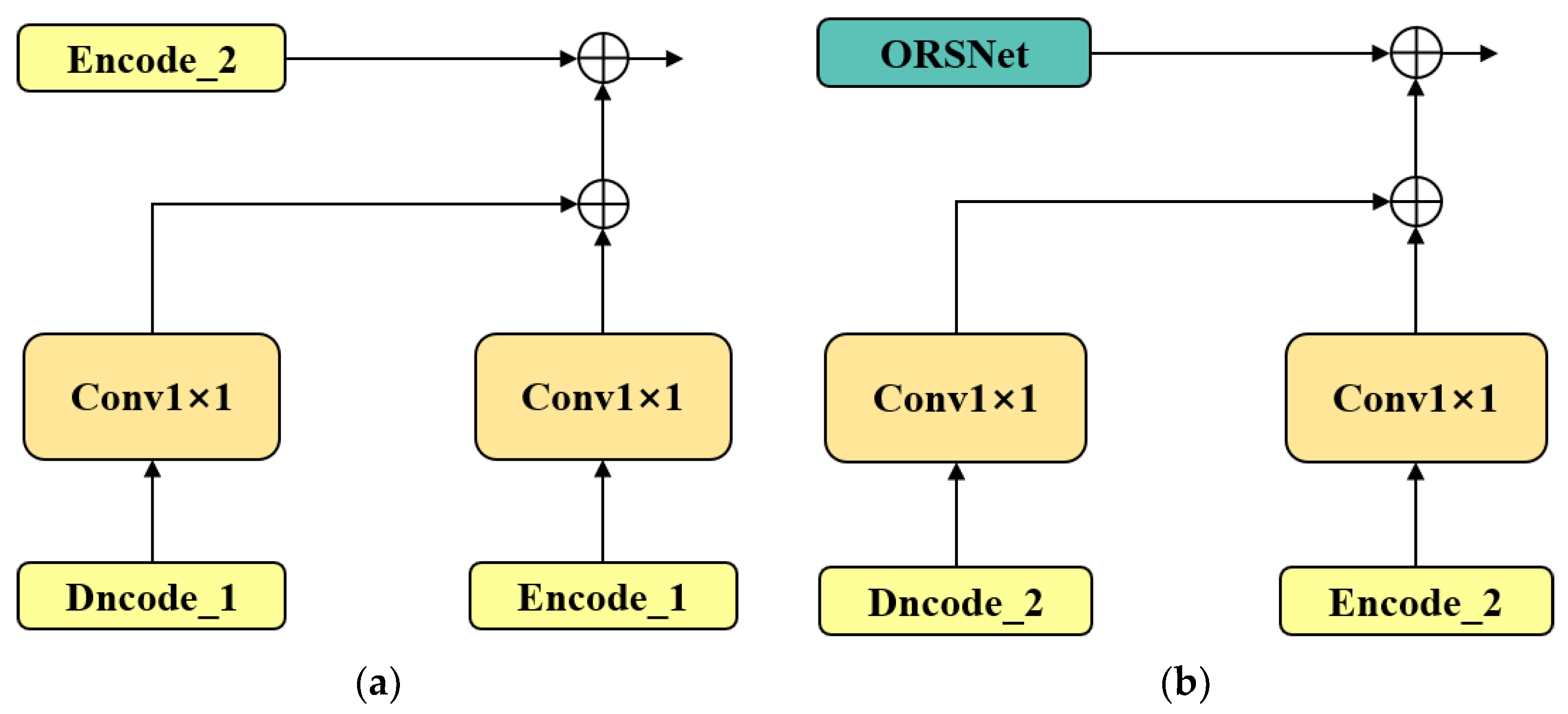
The MCFF module is introduced between the two encoder–decoders and between the encoder–decoder and ORSNet, in Figure 4. Before propagating the features of one stage to the next stage for aggregation, MCFF fuses the feature maps of the same size in the encoder and decoder of the previous stage into one feature map of the same size after 1 × 1 convolution, respectively. MCFF has three advantages.

• It can reduce the impact of information loss caused by repeated up-and-down sampling in the encoder–decoder.
• The multi-scale features of the previous stage can enrich the features of the next stage and retain more image details.
• It simplifies the flow of information and makes the network optimization process more stable.

3.3.4. Supervised Attention Module

Usually, the repairing results of the previous stage are directly transferred to the next stage, but the feature information passed to the next stage is not always useful for image repairing. Therefore, to convey useful feature information as much as possible, a supervised attention module is introduced between each stage. Providing the supervision of real images in the training phase of the network can filter useless feature information and train a better network model. The network structure diagram of SAM is shown in Figure 5. SAM inputs the inpainted image features $F_{\mathrm{in}}\in R^{H\times W\times C}$ of the previous stage, where H × W is the spatial dimension, and C is the number of channels. The residual image is added to the degraded input image I to obtain the restored image $X_{\mathrm{s}}\in R^{H\times W\times C}$. Real images can provide supervision that optimizes the repairing process. Next, the per-pixel attention masks $M_{\mathrm{a}}\in R^{H\times W\times C}$ are generated from the image $X_{\mathrm{s}}$ with 1 × 1 convolution and sigmoid activation. The input feature $F_{\mathrm{in}}$ is convolved using 1 x 1 convolution and then element-wise multiplied with the attention feature map. The attention feature map plays the role of controlling the input feature information to the next stage and inhibiting the transfer of less informative features to achieve the recalibration of features. Finally, the calibrated features are added to the input features as the output of SAM, which is passed to the next stage for repair.

3.3.5. Original Resolution Subnetwork

The final stage uses a subnetwork ORSNet that operates on the original input image resolution without any downsampling operation, so the desired fine texture is preserved in the final output image. ORSNet consists of multiple original resolution blocks, each of which contains channel attention blocks. An illustration of the original resolution block (ORB) in our ORSNet is shown in Figure 6.

3.3.6. Loss Function

To better repair the image, we use Charbonnier, edge loss, and generative adversarial loss functions to implement an end-to-end optimized multi-stage progressive repairing network:

$$L_{char}=\sqrt{||X_S-Y|{|}^2+{\epsilon }^2},$$

(9)

$$L_{edge}=\sqrt{||\Delta (X_S)-\Delta (Y)|{|}^2+{\epsilon }^2},$$

(10)

where $X_S$ is the directly predicted restoration image. It is the sum of the predicted residual image $R_S$ and the degraded input image I. Y is the real image, $L_{char}$ is the Charbonnier loss function, $\epsilon$ is empirically set to 10⁻³, $L_{edge}$ is the edge loss function, and $\Delta$ is the Laplacian operator.

Adversarial loss is widely used in the field of image repairing to improve the visual quality of image repairing. To stabilize the training of generative adversarial networks, we use a spectral normalized Markov discriminator:

$$L_{adv}=E_{Y~Pdata(Y)}[\mathrm{Re}LU(1-D^{\mathrm{sn}}(Y))]+E_{z~P_z(z)}[\mathrm{Re}LU(1+D^{\mathrm{sn}}(G(z)))],$$

(11)

where D^sn is the discriminator, G is the repairing network for the missing image z, and Y is the real image. Finally, the total loss function of the repair network is

$$L_{adv}=E_{Y~Pdata(Y)}[\mathrm{Re}LU(1-D^{\mathrm{sn}}(Y))]+E_{z~P_z(z)}[\mathrm{Re}LU(1+D^{\mathrm{sn}}(G(z)))],$$

(12)

where $\lambda$ is a parameter controlling the relative importance, which is set to 0.05.

3.4. The Pixel-Weighted Image Fusion Based on UCM

In order to equalize the gray value of the side-scan sonar image and add more details, we use the improved UCM pixel-weighted image fusion. Firstly, the repaired RGB side-scan sonar image is grayscale-corrected by UCM. Then, the repaired weighted grayscale sonar image and the grayscale corrected RGB image are weighted fused, and the weighting coefficients are obtained through multiple experiments to increase the details of the image while avoiding adding more noise.

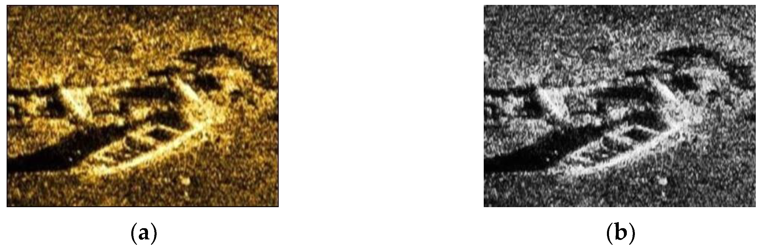
3.4.1. The Improved Unsupervised Color-Correction Method

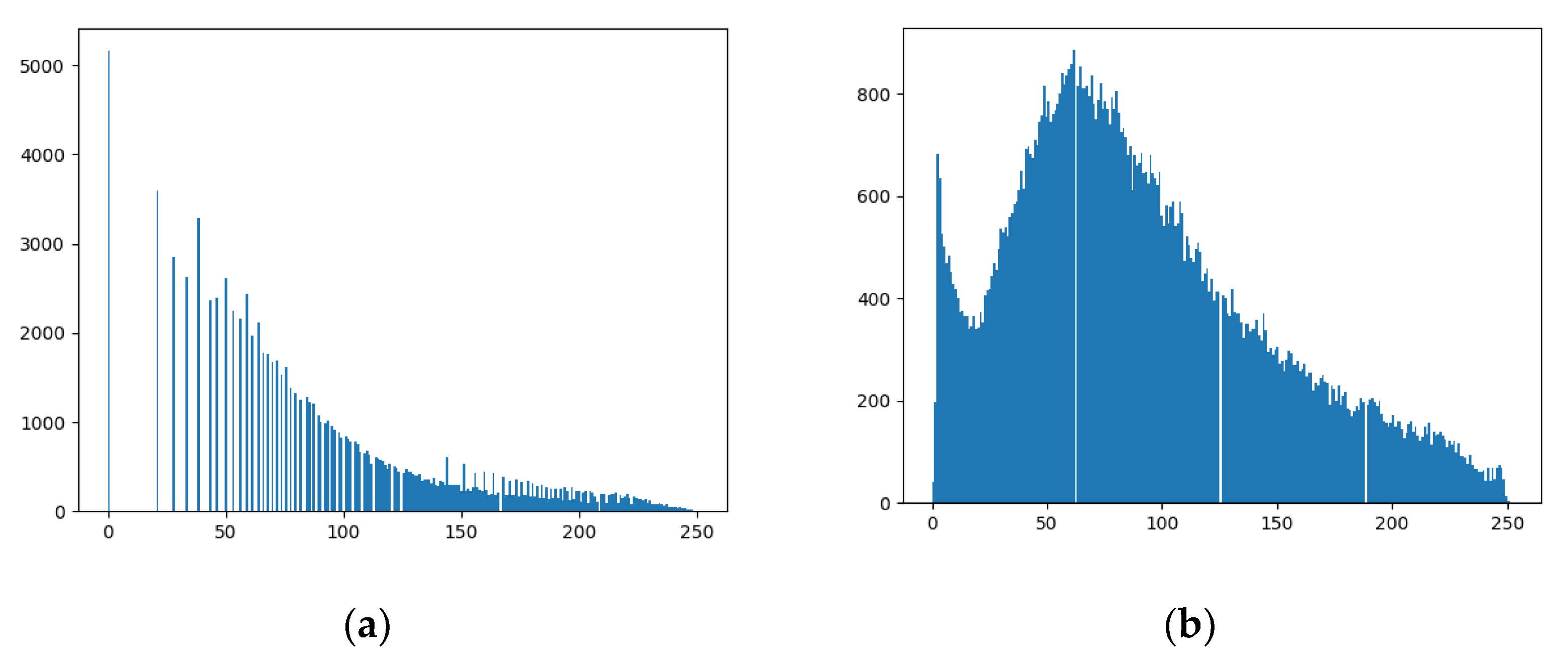
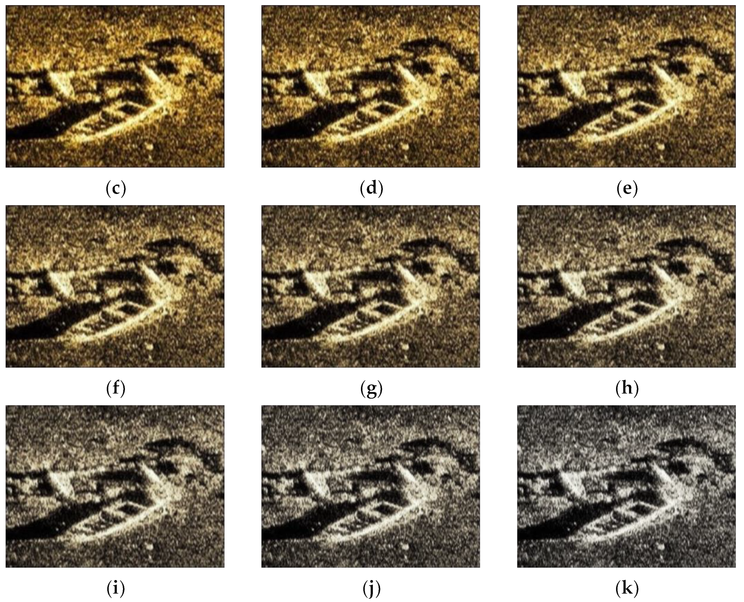
In general, the original image of the side-scan sonar is dull and monotonous, and its gray histogram is distributed in a relatively low range and relatively concentrated. However, the gray values of the histogram of the sonar image corrected by improved UCM are evenly distributed, as shown in Figure 7.

Other common grayscale correction methods are not used because the color of the original sonar image will be changed, as shown in Figure 8. The traditional UCM method is mainly applied to the color-correction problem of underwater images [19,20], but there is no such problem in side-scan sonar images. Therefore, UCM is improved by deleting the gain factor that corrects the underwater color cast. The improved UCM algorithm is divided into three steps. The colors are first equalized by white balance. Then, the histogram of R, G, and B channels in the RGB color model is linearly stretched to improve the contrast. Finally, the histogram of S and I channels in the HIS color model is linearly stretched to increase the true color and brightness. The steps are as follows:

• Equalization of RGB color models. The average values of R, G, and B channels in the image are calculated, as shown in Equation (10), where $I_R\left(i,j\right)$, $I_G\left(i,j\right)$, and $I_B\left(i,j\right)$ are the pixel values of red, green, and blue channels on an image of size M × N, respectively. $i=1,2,\cdots ,M$, $j=1,2,\cdots ,N$;

  $$\left\{\begin{array}{c}{R}_{avg}=\frac{1}{MN}{\displaystyle \sum _{i=1}^M{\displaystyle \sum _{j=1}^N{I}_R\left(i,j\right)}}\\ G_{avg}=\frac{1}{MN}{\displaystyle \sum _{i=1}^M{\displaystyle \sum _{j=1}^N{I}_G\left(i,j\right)}}\\ B_{avg}=\frac{1}{MN}{\displaystyle \sum _{i=1}^M{\displaystyle \sum _{j=1}^N{I}_B\left(i,j\right)}}\end{array}\right.,$$

  (13)
• RGB color model contrast correction. After balancing the color of the image in Step 1, the improved UCM algorithm further improves the contrast of the sonar image. The correction of contrast is mainly stretching the pixel value range of the three channels R, G, and B to the desired range. Typically, the value of the 8-bit color channel varies from 0 to 255. The stretching formula of this method is a linear stretching function, as shown in Equation (14), where p₀ is the pixel value of the output image, p_i is the pixel value of the input image, a and b are the minimum and maximum pixel values in the image, and c and d are the stretch parameters, which are generally set to 255 and 0;

  $$p_0=(p_i-a)(\frac{c-d}{b-a})+d,$$

  (14)
• Saturation and brightness correction for HSI color models. The RGB color model processed in Step 1 and Step 2 is converted into the HSI color model, where H represents the hue, S represents the saturation, and I represent the brightness. By stretching the S and I channels to each side, we can expand the distribution of the histogram. It further increases the true color by increasing the saturation, and it solves the low light problem by increasing the brightness to make the processed image more natural.

3.4.2. Pixel-Weighted Image Fusion

RGB images provide color information, and grayscale images have more details [21]. Therefore, the goal of fusion is to obtain a color image that preserves the color of the image but has more details. In this way, the processed image can be balanced in contrast and color restoration to achieve the desired enhancement effect.

We use the pixel-weighted fusion method. The RGB sonar image with improved UCM grayscale correction and the repaired weighted grayscale sonar image is fused with weights of 0.9 and 0.1, respectively. The fused image should not only preserve the contrast of the image, but also correct the color. If other values are used, the enhanced image may have insufficient color correction or insufficient image contrast enhancement.

4. Experimental Results and Analysis

In this section, the performance of adaptive Gaussian denoising and pixel-weighted image fusion will be verified by experiments. Experiments were conducted to compare the proposed algorithm with the commonly used side-scan sonar image enhancement methods. We will evaluate from subjective feeling, contrast, brightness, color correction, and other aspects. The image quality evaluation criteria, including information entropy, MSE, PSNR, and SSIM, were objectively analyzed to comprehensively evaluate the enhanced image. All experiments were performed on a PC of 4GRAM and 2.4 GHz.

4.1. Side-Scan Sonar Image Data

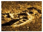
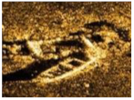
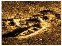
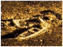
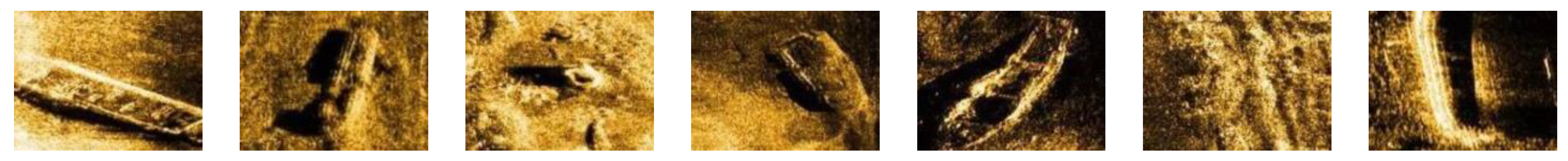
Part of the experimental images are examples of shipwrecks taken within rivers in China in the high-speed mode of multibeam side-scan sonar from Beijing Lanchuang Ocean Technology Co. The data images contain different types of shipwrecks. The target wreck area is compared with the background area, and it is found that the side-scan sonar images suffer from a severe imbalance between target and background pixels and contain reverberant noise on the seafloor. The other experimental images are from the side-scan sonar images acquired by Marine Sonic Technology and the United States Geological Survey. Due to the large size of the side-scan sonar image, the image was cropped into 368 × 273 pixel blocks. Finally, a total of 980 valid data images were summarized and analyzed. Part of the side-scan sonar images is shown in Figure 8.

4.2. Performance of Adaptive Gaussian Filtering

The comparison in

Table 1. Comparison of Gaussian filtering effect.

Method	Figure	PSNR
Traditional		20.43
Adaptive		23.50

shows that the improved adaptive Gaussian filtering method has a better visual effect, and the PSNR is improved by 15%.

4.3. Performance of Convolutional Block Attention Module

The commonly used attention mechanisms were studied: channel attention mechanism (SE-Net), spatial attention mechanism (STN), and hybrid spatial and channel attention mechanism (CBAM). Among them, SE-Net consists of two parts, squeeze and excitation, which can enhance important channels, capture global information, and have small computational costs, but they lack local information, high model complexity, and computational time; STN has transformation invariance but relies on high-quality data, a limited range of image transformations, and high computational cost with high training complexity; CBAM can adapt to different sizes of access and has rich channel and spatial feature information, but it focuses too much on local features [22]. All of the above methods have their advantages and disadvantages, so the above attention mechanisms are added to the algorithm, and the overall performance of the final image processing is compared.

From

Table 2. Performance comparison of attention modules.

Method	Figure	PSNR	TIME
SE-Net		25.568	65.2 s
STN		26.837	61.7 s
CBAM		27.243	71.5 s

, it can be seen that among the available data images, using CBAM to process the image localization effect and PSNR is better, but the running time is worse than the other two; however, considering the de-drying effect is the best, this attention mechanism module is used. In future research, we will continue the research on CBAM to improve the running speed.

4.4. Performance of Pixel-Weighted Image Fusion Based on Improved UCM

Figure 7 shows that the gray values of the histogram of the sonar image corrected by improved UCM are evenly distributed.

Figure 9 shows the effect comparison of different pixel-weighted fusion coefficients of improved UCM processes in the image and grayscale image repaired. The value of a represents the pixel weight of Figure 9a, and the value of b represents the pixel weight of Figure 9b. After several experiments, the pixel weight coefficients with weights of 0.9 and 0.1 are selected. The fused image should not only preserve the contrast of the image, but also correct the color. If other values are used, the enhanced image may have insufficient color correction or insufficient image contrast enhancement.

According to the comparison of data before and after pixel-weighted fusion in

Table 3. Comparison before and after fusion using pixel-weighted image fusion.

Method	PSNR	SSIM
No pixel-weighted image fusion	26.984	0.952
Pixel-weighted image fusion	27.243	0.956

, we can know that PSNR is increased by 0.95% and SSIM is increased by 0.42%.

4.5. Overall Algorithm Effect Analysis

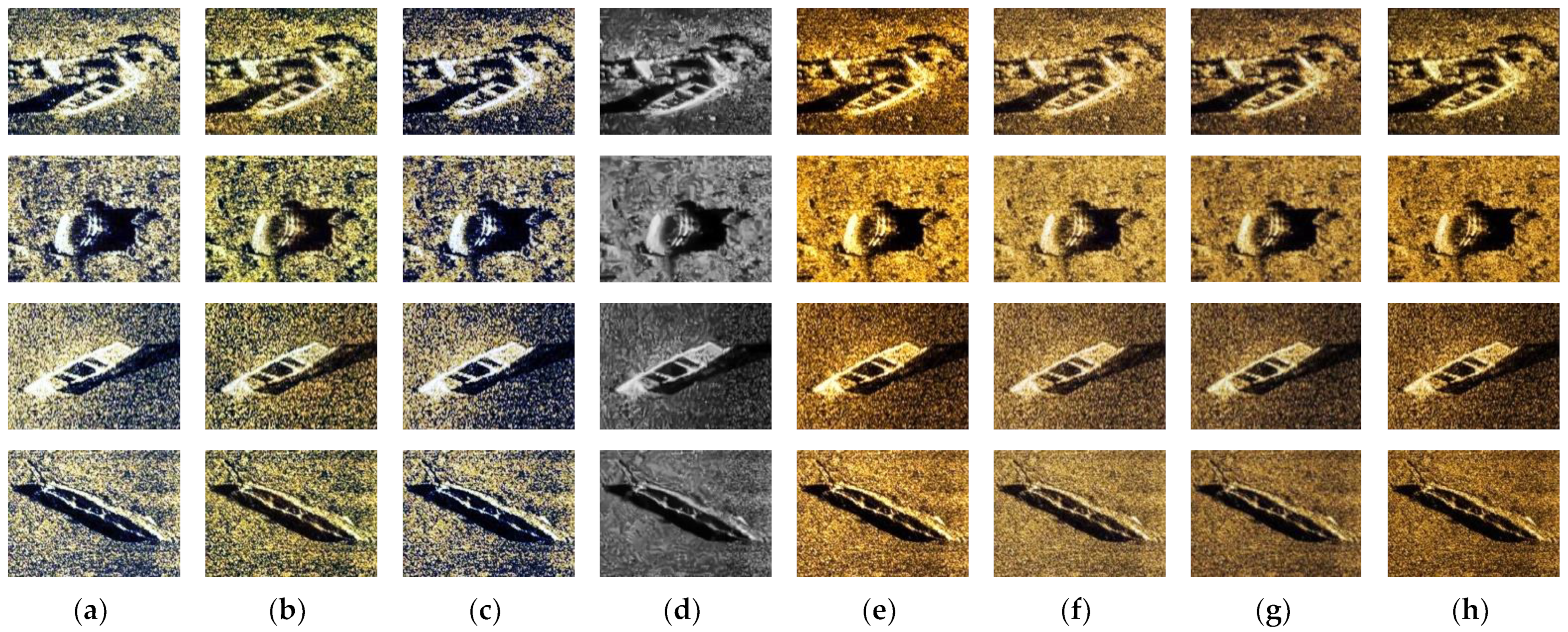
4.5.1. Subjective Analysis

As show in Figure 10, the sharpness of HE, CLAHE, Rayleigh, and BM3D enhancement is very poor. Among them, HE, CLAHE, Rayleigh, and BM3D change the color of the original sonar image, and cause image blur and overcorrection after correction with the BM3D method. The contrast and brightness of the images enhanced using the RGHS method are too high. Compared with these methods, Retinex, GAN, and our enhancement algorithm has a better balance among chroma, saturation, and contrast, and the processed image is more consistent with human visual perception and is clearer and more stable.

4.5.2. Objective Analysis

In order to evaluate the image enhancement algorithm more fairly, the image quality evaluation indicators, including information entropy, MSE, PSNR, and SSIM, were used to evaluate the enhanced side-scan sonar images. Higher information entropy indicates clearer images and higher PSNR scores, and lower MSE scores indicate that the results are closer to the reference image in terms of image content, while higher SSIM scores mean that the results are more similar to the reference image in terms of image structure and texture.

According to

Table 4. Image quality assessment metrics.

Image	Method	Entropy	PSNR	SSIM	MSE
Image 1	HE	7.847	12.943	0.698	3301.756
	CLAHE	7.767	16.345	0.779	1508.438
	RGHS	7.702	24.079	0.944	254.189
	GAN	7.852	21.514	0.804	458.755
	BM3D	7.559	15.664	0.608	1764.586
	Retinex	7.779	19.362	0.870	753.174
	Ours	7.857	27.243	0.956	122.653
Image 2	HE	7.945	12.613	0.697	3562.527
	CLAHE	7.968	15.893	0.764	1674.00
	RGHS	7.281	20.349	0.946	600.01
	GAN	7.895	20.306	0.812	423.566
	BM3D	7.432	13.420	0.580	2958.080
	Retinex	7.586	19.279	0.882	767.589
	Ours	7.874	31.055	0.967	50.996
Image 3	HE	7.953	11.237	0.610	4890.696
	CLAHE	7.915	15.479	0.713	1841.199
	RGHS	7.756	24.496	0.966	230.884
	GAN	7.882	22.302	0.792	480.785
	BM3D	7.364	17.244	0.638	1226.425
	Retinex	7.697	19.041	0.861	810.842
	Ours	7.727	27.622	0.928	112.412
Image 4	HE	7.939	11.639	0.637	4457.708
	CLAHE	7.949	15.670	0.733	1762.108
	RGHS	7.662	17.854	0.883	1065.609
	GAN	7.913	23.008	0.828	452.526
	BM3D	7.096	15.425	0.581	1864.452
	Retinex	7.514	18.005	0.857	1029.203
	Ours	7.650	26.469	0.911	146.591

, our algorithm has the highest entropy, PSNR, and SSIM and the lowest MSE. Compared with the method with the best evaluation index, the evaluation index optimization is shown in the table below.

Integrating all the side-scan sonar data, compared with the algorithm with the best evaluation index, the proposed algorithm improves PSNR by 26.58%, SSIM by 0.68%, and MSE by 65.02% on average. It shows that the sonar image enhanced by the proposed method is clearer, the ability to suppress noise is stronger, and the image information is richer.

5. Conclusions

Since the original side-scan sonar image is affected by grayscale distortion and environmental noise, image enhancement is required before further image processing. We propose a side-scan sonar image enhancement method based on multi-stage repairing image fusion, which is simple and easy to implement. Among them, the adaptive Gaussian filtering algorithm maliciously suppresses speckle noise from the environment in side-scan sonar images to a greater extent. The feature information is efficiently extracted using ARFM, and the interaction is fused using MCFF in a multi-stage repair network. The pixel-weighted image fusion method based on UCM corrects the image grayscale while ensuring the image details.

Compared with the commonly used side-scan sonar image enhancement methods, our method can effectively correct the gray distortion in side-scan sonar images and avoid the shortcomings of a single denoising algorithm that cannot effectively equalize the gray values. The images processed by our image enhancement algorithm are balanced in terms of chroma, contrast, and saturation and are grayscale balanced, which is in line with human visual perception. Compared with the algorithm with the SOTA methods on datasets, the PSNR is increased by 26.58%, the SSIM is increased by 0.68%, and the MSE is reduced by 65.02% on average.

References

- Ye, X.; Yang, H.; Li, C.; Jia, Y.; Li, P. A Gray Scale Correction Method for Side-Scan Sonar Images Based on Retinex. Remote Sens. 2019, 11, 1281. [Google Scholar] [CrossRef]
- Ye, X.; Yang, H.; Jia, Y.; Liu, J. Geometric Correction Method of Side-Scan Sonar Image. In Proceedings of the OCEANS, Marseille, France, 17–20 June 2019. [Google Scholar]
- Ge, Q.; Ruan, F.; Qiao, B.; Zhang, Q.; Zuo, X.; Dang, L. Side-Scan Sonar Image Classification Based on Style Transfer and Pre-Trained Convolutional Neural Networks. Electronics 2021, 10, 1823. [Google Scholar] [CrossRef]
- Kapetanović, N.; Mišković, N.; Tahirović, A. Saliency and Anomaly: Transition of Concepts from Natural Images to Side-Scan Sonar Images. IFAC-PapersOnLine 2020, 53, 14558–14563. [Google Scholar] [CrossRef]
- Grabek, J.; Cyganek, B. Speckle Noise Filtering in Side-Scan Sonar Images Based on the Tucker Tensor Decomposition. Sensors 2019, 19, 2903. [Google Scholar] [CrossRef] [PubMed]
- Kim, K.; Intrator, N.; Neretti, N. Image Registration and Mosaicing of Noisy Acoustic Camera Images. In Proceedings of the 11th IEEE International Conference on Electronics, Circuits and Systems, Tel Aviv, Israel, 13–15 December 2004; pp. 527–530. [Google Scholar]
- Burguera, A.; Oliver, G. Intensity Correction of Side-Scan Sonar Images. In Proceedings of the 19th IEEE International Conference on Emerging Technology and Factory Automati on (ETFA), Barcelona, Spain, 16–19 September 2014. [Google Scholar]
- Shi, P.; Lu, L.; Fan, X.; Xin, Y.; Ni, J. A Novel Underwater Sonar Image Enhancement Algorithm Based on Approximation Spaces of Random Sets. Multimed. Tools Appl. 2021, 81, 4569–4584. [Google Scholar] [CrossRef]
- Shippey, G.; Bolinder, A.; Finndin, R. Shade Correction of Side-Scan Sonar Imagery by Histogram Transformation. In Proceedings of the OCEANS’94, Brest, France, 13–16 December 2002; pp. 439–443. [Google Scholar]
- Mehmet, Z.K.; Erturk, S. Enhancement of Ultrasound Images with Bilateral Filter and Rayleigh CLAHE. In Proceedings of the 23nd Signal Processing and Communications Applications Conference (SIU), Malatya, Turkey, 16–19 May 2015; pp. 1861–1864. [Google Scholar]
- Chang, Y.C.; Hsu, S.K.; Tsai, C.H. Sidescan sonar image processing: Correcting Brightness Variation and Patching Gaps. J. Mar. Sci. Technol. 2010, 18, 785–789. [Google Scholar] [CrossRef]
- Huang, D.; Wang, Y.; Song, W. Shallow-Water Image Enhancement Using Relative Global Histogram Stretching Based on Adaptive Parameter Acquisition. MultiMedia Model. 2018, 10704, 453–465. [Google Scholar]
- Chang, C.; Hsiao, J.; Hsieh, C. An Adaptive Median Filter for Image Denoising. In Proceedings of the 2008 Second International Symposium on Intelligent Information Technology Application, Shanghai, China, 20–22 December 2008. [Google Scholar]
- Zhang, C.; Bai, L.; Zhang, Y.; Zhang, B. Hierarchical Image Fusion Based on Wavelet Transform. In Proceedings of the IEEE International Conference on Mechatronics and Automation, Luoyang, China, 25–28 June 2006. [Google Scholar]
- Chen, G.; Xie, W.-F.; Dai, S. Image Denoising with Signal Dependent Noise Using Block Matching and 3D Filtering. In Proceedings of the 11th International Symposium on Neural Networks (ISNN), Hong Kong and Macao, China, 28 November–1 December 2014; pp. 423–430. [Google Scholar]
- Mozerov, M.G.; van de Weijer, J. Global Color Sparseness and a Local Statistics Prior for Fast Bilateral Filtering. IEEE Trans. Image Process. 2015, 24, 5842–5853. [Google Scholar] [CrossRef] [PubMed]
- Kotecha, J.H.; Djuric, P.M. Gaussian Particle Filtering. IEEE Trans. Signal Process. 2003, 51, 2592–2601. [Google Scholar] [CrossRef]
- Chen, Q.; Wu, D. Image Denoising by Bounded Block Matching and 3D Filtering. Signal Process. 2010, 90, 2778–2783. [Google Scholar] [CrossRef]
- Banić, N.; Lončarić, S. Unsupervised Learning for Color Constancy. In Proceedings of the 13th International Joint Conference on Computer Vision, Imaging and Computer Graphics Theory and Applications (VISIGRAPP 2018), Funchal, Portugal, 27–29 January 2018; pp. 181–188. [Google Scholar]
- Oliveira, M.; Sappa, A.D.; Luo, J. Unsupervised Local Color Correction for Coarsely Registered Images. In Proceedings of the IEEE Conference on Computer Vision and Pattern Recognition (CVPR), Colorado Springs, CO, USA, 20–25 June 2011; pp. 201–208. [Google Scholar]
- Zhang, Y.; Bai, X.; Wang, T. Boundary Finding Based Multi-Focus Image Fusion through Multi-Scale Morphological Focus-Measure. Inf. Fusion 2017, 35, 81–101. [Google Scholar] [CrossRef]
- Zamir, S.W.; Arora, A.; Khan, S. Multi-Stage Progressive Image Restoration. In Proceedings of the Computer Vision and Pattern Recognition, Virtual, 19–25 June 2021; pp. 14816–14826. [Google Scholar]