Research on Earthquake Data Prediction Method Based on DIN–MLP Algorithm

Abstract

This paper proposes a recommendation algorithm that combines MLP with the DIN model and conducts simulation experiments in the field of earthquake missing data prediction. The original DIN model may face challenges and weaknesses in earthquake monitoring data prediction, such as a limited capability in handling data loss or anomalies in seismic monitoring stations. To overcome these issues, we innovatively treat seismic monitoring stations as special users and historical data patterns as recommended items. Based on the DIN model, we implement data processing and prediction for seismic monitoring stations and introduce an attention mechanism based on MLP neural networks in the model, while leveraging the prior knowledge base to enhance predictive capabilities. Compared to the original DIN model, our proposed approach not only recommends sequence combinations that meet the demands of seismic monitoring stations but also enhances the matching between station behavior attributes and historical data characteristics, thereby significantly improving prediction accuracy. To validate the effectiveness of our method, we conducted comparative experiments. The results show that the GAUC achieved by the DIN–MLP model reaches 0.69, which is an 11 percent point improvement over the original DIN model. This highlights the remarkable advantages of our algorithm in earthquake missing data prediction. Furthermore, our research reveals the potential of the DIN–MLP algorithm in practical applications, providing more accurate data processing and time series combination recommendations for the field of earthquake monitoring stations, thus contributing to the improvement of monitoring efficiency and accuracy.

1. Introduction

In the process of earthquake monitoring, due to various reasons such as instrument failure and communication failure, some data may be lost. The problem of multiple fields’ continuous missing values or the appearance of singular values in earthquake monitoring data reflects this issue, which will have a serious impact on subsequent data analysis and business applications [1]. Due to the complexity of the geographical location distribution of earthquake monitoring stations and the uncertainty of hardware equipment repair, maintenance work cannot be completed in a short time. Therefore, during the period when the monitoring station cannot operate normally, how to use technical methods to complete the missing data and ensure data integrity is a practical and meaningful issue. However, the hardware equipment and observed data of earthquake monitoring stations vary greatly. For example, seismograph stations primarily use seismographs to collect vibration data, whereas geomagnetic and geoelectric monitoring stations rely on magnetometers or voltmeters. Crustal stress, geotemperature, and atmospheric pressure monitoring stations require specialized sensors to detect subtle changes in these parameters. Because the nature of the data observed by different stations, as well as the scale and structure of the data, differ, a single completion algorithm may not apply to all types of observation data. Therefore, an effective method is needed to predict and complete the missing data of a station according to the specific hardware equipment and characteristics of the observed data of that earthquake monitoring station.

To address this issue, one possible solution is to develop an algorithm that can effectively predict and complete missing data in seismic monitoring stations. However, due to the significant differences in hardware configurations and data characteristics among seismic stations, creating customized algorithms for each station presents a tremendous challenge. Therefore, we need to design a mechanism that can learn the historical data patterns of each station from the prior knowledge base based on their unique characteristics and requirements. This mechanism will then match each station with the corresponding prior model that aligns with its features, enabling data prediction and completion. Priori models refer to models established based on prior experiences or existing knowledge to perform data prediction, completion, or other machine learning tasks. These priori models analyze the commonalities and differences among stations, learning the unique characteristics and data patterns of each station. Consequently, they are matched with stations having similar data patterns, enabling better data prediction and completion.

The purpose of this paper is to improve the accuracy and interpretability of seismic monitoring station data prediction by integrating the Multilayer Perceptron (MLP) with the Deep Interest Network (DIN) model and making full use of prior knowledge. This will provide more accurate time series combinations for seismic monitoring stations, thus enhancing the efficiency and accuracy of seismic monitoring. To achieve this goal, we propose the DIN–MLP model. The main contributions of this paper are as follows:

• Combining the MLP with the DIN model, we propose a novel recommendation algorithm aimed at addressing the challenges of data loss or anomalies in seismic monitoring;
• We introduce an innovative approach that treats seismic monitoring stations as special users and historical data patterns as recommended items. This method allows us to learn the historical data patterns of each station from the prior knowledge base, matching each station with a relevant prior model based on its unique characteristics and requirements for data prediction and completion;
• The DIN model is enhanced by incorporating an attention mechanism based on the MLP neural network. This attention mechanism improves the matching between station behavior attributes and historical data features, thereby enhancing prediction accuracy;
• Experimental results demonstrate that the proposed model outperforms the original DIN model. The new model not only improves prediction accuracy but also ensures diverse and reliable recommendations. This diversity is crucial for providing comprehensive and trustworthy predictions in seismic monitoring.

The remaining structure of this paper is as follows. In Section 2, we provide an overview of the research status in the fields of seismic missing data and recommendation algorithms. In Section 3, we introduce the design and structure of the proposed model, followed by improvements in Section 4. Section 5 presents the simulation experiments and data analysis. Finally, in Section 6, we summarize the entire paper.

2. Related Theory and Methods

2.1. Current Status of Intelligent Completion of Missing Seismic Data

Seismic data completion has been a long-standing research topic in the field of seismic data processing. During the seismic data collection process, due to economic constraints, geological conditions, and other factors, the obtained seismic data often contain regular or irregular missing traces. This severely impacts subsequent seismic data processing and interpretation, such as offset imaging and full waveform inversion. To improve the completeness and quality of seismic data, it is necessary to interpolate and reconstruct the missing seismic data.

Deep learning, a popular technology in recent years, has been widely used in the field of geophysics. Deep learning-based seismic data reconstruction methods are mainly divided into three categories: supervised, unsupervised, and self-supervised methods. Mandelli et al. [2] used a convolutional autoencoder to reconstruct the missing traces of pre-stack seismic data and achieved good results. Park et al. [3] developed a reconstruction method for regularly missing seismic data using the U-Net network widely used in the medical field. Wang et al. [4] trained a residual network to reconstruct regular and irregularly missing seismic traces. Li et al. [5] proposed a U-net network structure, with a coordinate attention block for reconstructing two-dimensional seismic data. Yu and Wu [6] proposed a method with a mixed loss function and attention mechanism-guided convolutional neural network to reconstruct continuously missing seismic traces. Jiang et al. [7] proposed a new focal frequency loss, optimizing the network model directly in the frequency domain to further improve the image reconstruction quality. All the deep learning-based methods mentioned above are supervised learning methods, and their excellent performances depend on the ability to learn the mapping between missing data and complete data through sufficient labels. However, in practical applications, it is challenging to obtain a large amount of complete seismic data. To address this problem, Xu et al. [8] proposed a new “Noisy as Clean” strategy for the denoising task, training a self-supervised image denoising network and avoiding the use of labeled data for training. Fei et al. [9] proposed a “Missing-As-Complete” (MAC) strategy to train the network to solve the problem of missing target labels in practical situations. Chen et al. [10] used a dropout layer to perform random Bernoulli sampling of the original missing seismic data to make a training set, using only known seismic traces for deep neural network training, thereby achieving unsupervised seismic data reconstruction. Meng et al. [11] proposed an unsupervised deep learning method based on residual networks for reconstructing missing seismic data. This approach involves using random data as input and seismic data with missing traces as the desired output. The network parameters are optimized to minimize the error, aiming to obtain an optimal network configuration.

2.2. Research Status of Recommendation Algorithms

2.2.1. Traditional Recommendation Algorithms

Traditional recommendation techniques include collaborative filtering recommendations, content-based recommendations, and hybrid recommendation algorithms. These three algorithms are introduced separately as follows.

Collaborative filtering recommendation algorithms are the earliest recommendation algorithms. They mainly use the user’s historical behavior information to derive a score matrix of items with which the user has interacted and then easily find similar users or items through suitable similarity calculation methods. Finally, the list of recommendations to the user is extracted from similar information [12]. This algorithm is suitable for small-scale recommendations and is simple and easy to operate; however, it has a cold start problem and lacks the interpretability of recommendations. To address the cold start problem in traditional collaborative filtering algorithms, Liu et al. [13] proposed a novel algorithm based on user clustering. This algorithm pre-fills the user–item rating matrix and takes into account both the user features and scores when computing user similarity. Additionally, an optimized K-means algorithm is employed for user clustering. Nataralan et al. [14] devised a recommendation system model named RS-LOD (Recommendation System-Linked Open Data) to tackle the cold start problem. This model utilizes linked open data, which may contain relevant attribute information about users or items to enhance recommendation performance. By leveraging this attribute information, RS-LOD gains a better understanding of the relationships between users and items, enabling more accurate recommendations in cold start scenarios. Furthermore, user attribute information is applied to improve similarity calculation in recommendations and alleviate the cold start problem [15].

The principle of content-based recommendation systems [16] is relatively simple. After users generate historical behaviors, they interact with items they are interested in. These interactions can be seen as the users’ ratings of items. Based on the rated items, the user-rated items and other items are calculated for similarity, and the similar items form the recommended list for the user. This can solve the cold start problem but lacks feature extraction methods. Typical content-based recommendation systems include WebPersonalizer from DePaul University and CiteSeer from NEC Research Institute [17].

Hybrid recommendation [18] is not a specific recommendation algorithm, but rather an organic combination of existing recommendation methods. By using multiple recommendation algorithms for recommendation and leveraging their strengths, better recommendation results can be achieved. Real world recommendation scenarios are often complex and require tailored recommendation strategies for different recommendation problems. This approach helps to compensate for the shortcomings of different techniques but lacks an efficient blending mode. To improve prediction accuracy, R. Logesh et al. [19] proposed a tailored context-aware hybrid travel recommendation framework based on user qualitative knowledge and opinion-mining techniques. R. Kiran et al. [20] introduced a novel deep learning hybrid recommendation algorithm that utilizes embeddings to represent users and items, enabling the learning of nonlinear latent factors. The algorithm addresses the cold start problem, by incorporating certain user or item data into a deep neural network. Zafran Khan et al. [21] presented a deep semantic-based topic-focused hybrid recommendation model for a hybrid recommendation system. This system incorporates semantically defined items inspired by topic content to enhance the recommendations.

2.2.2. Deep Learning-Based Recommendation Algorithms

Deep learning, as a powerful intelligent algorithm, can autonomously learn and handle complex problems like humans when facing massive data. When dealing with linear or nonlinear feature sequences, it can not only analyze and calculate from multiple dimensions but also automatically extract features that meet user needs from a large amount of data. Deep learning technology can not only discover the potential feature representations hidden in user behavior records, but also capture the interaction features of nonlinear relationships between various subjects, which improves the recall and accuracy of the system, overcomes the shortcomings in traditional recommendation techniques, and achieves more accurate recommendations.

Sun et al. [22] proposed a collaborative filtering-based sampling recommendation algorithm (CFSR) that automatically recommends samples with defective data. They combined multi-criteria recommendation with deep learning collaborative filtering to enhance recommendation performance. Xiong et al. [23] introduced a deep learning-based hybrid web service recommendation approach that combines collaborative filtering with text content to recommend relevant web services. Covington et al. [24] were the first to apply the deep neural network model to the field of YouTube video recommendations, effectively absorbing many signals through the deep collaborative filtering model and using deep learning to model their interactions. The experiments prove that the performance of this method is superior to the matrix decomposition used by YouTube previously. The recommendation process is divided into two stages: candidate set generation and video sorting. This recommendation flow is shown in Figure 1.

The first stage is conducted by the candidate generation network, which takes user YouTube activity history events as input and retrieves a small subset (a few hundred) of videos from a large corpus. These candidate objects are aimed to be highly relevant to the user with high precision. The candidate generation network only provides broad personalization through collaborative filtering. User similarity is represented with coarse features, such as the video IDs watched, search query tokens, and demographic data. In the second stage, the ranking network accomplishes this task by using a set of rich features describing both the videos and users. It assigns scores to each video, based on the desired objective function. The videos with the highest scores are presented to the user and ranked accordingly. Although the proposed model can make predictions on large-scale data and exhibits some advantages in terms of computational efficiency compared to similar models, it has a simplified data processing process, which may lead to overfitting. To address this, attention mechanisms can be introduced to assign different weights to different data during the data processing stage.

3. DIN Model Based on Feature Learning and Prior Knowledge Base Pattern Recommendation

In situations where it is necessary to combine the recommendation business of the prior knowledge base with time series prediction tasks, traditional recommendation techniques cannot meet the business needs of this study due to their simplistic theoretical foundations. In contrast, algorithms such as CNN (Convolutional Neural Networks), GNN (Graph Neural Networks), and RNN (Recurrent Neural Networks) are better suited to processing image and text data. However, most of the data related to this study, such as the hardware and software configurations of seismic monitoring equipment and behavior patterns, are discrete and continuous variables. These models cannot fully exploit the potential relationships within these data, making it difficult to meet the requirements of time series prediction tasks. The original intention of the DIN (Deep Interest Network) model design is to explore the relationship between user behavior and product attributes. In the context of this study, we can consider seismic monitoring devices as a specialized “user” group and various potential prior models as available “items” or “products”. We can use the attention mechanism to find the relationship between the two and recommend suitable “products” to them.

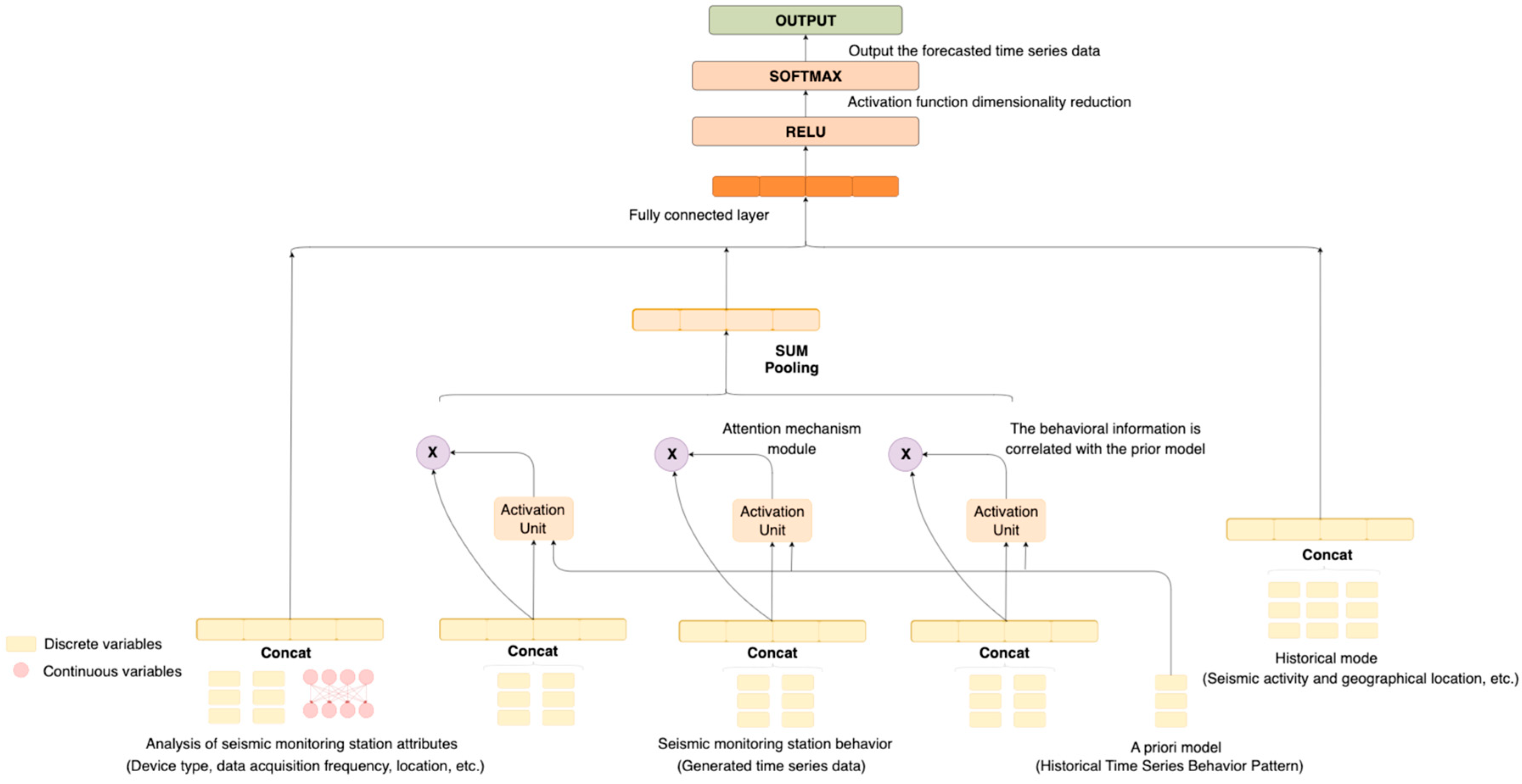
Therefore, this study uses the DIN model to complete the pattern recommendation of the prior knowledge base and improves it. The structure of the DIN model is shown in Figure 2. The input of this model is the original data collected by the seismic monitoring equipment and the prior model, and the output is the predicted time series.

This model is a recommendation model, implemented based on neural networks, and when applied to the time series prediction of seismic stations, it fully utilizes various information to realize prediction services. In this scenario, station attributes such as ID, behavior, and working hours are transformed into corresponding feature vectors through an embedding layer, resulting in station feature vectors. Prior models (such as previously learned time series patterns) are also transformed into feature vectors through an embedding layer, generating model feature vectors. Simultaneously, station behavior and prior models are mapped into high-dimensional vectors. By leveraging the powerful learning representation capabilities of attention mechanisms and neural networks, we can capture the nonlinear interaction between station behavior and prior models, uncovering deep-level relationships. This model outputs a predicted feature vector, which is then fully connected with the station attributes to generate a predicted time series list and scores.

However, it is worth noting that the original one-dimensional time series data cannot be directly used for this model and need to be processed accordingly. The following sections will introduce this process and each part of this model.

3.1. Conversion of One-Dimensional Time Series to Two-Dimensional Tensors

To better mine the structure and patterns in seismic data to extract valuable features, we need to convert the collected one-dimensional time series data into a two-dimensional tensor. The original one-dimensional time series can be represented as $X\left(t\right)$, where $t=\{0,1,\dots ,\mathrm{T}-1\}$, and $X\left(t\right)$ represents the data point at time $t$. Subsequently, we divide the time series into equal intervals, assuming that the length of each interval is $N$, and then we can obtain $M=T/N$ time series segments as follows: $\left\{X_0\right(t),X_1(t),\dots ,X_{M-1}(t\left)\right\}$. Each $X_i\left(t\right)$ (where i = 0, 1, …, M − 1 and t = 0, 1, …, N − 1) represents the time series in the i-th segment, and each data point within it can be seen as a feature that needs to be encoded as a vector.

Firstly, each data point in the time series needs to be standardized to eliminate the impact of the different scales of different features. In this process, the value of each data point will be standardized by the mean and standard deviation of its corresponding time segment. Specifically, suppose that the data point at time $t$ in the i-th time series segment is $X_i\left(t\right)$. We can calculate the mean ${\mu }_i$ and standard deviation ${\sigma }_i$ for this time segment, then obtain the standardized data point, as shown in Equation (1):

$$Z_i\left(t\right)=\frac{(X_i\left(t\right)-{\mu }_i)}{{\sigma }_i}$$

(1)

Next, we will combine all the standardized data points within each time segment to form a one-dimensional vector of length $N$, that is, $Z_i=\left[Z_i\right(0);Z_i(1);\dots ;Z_i(N-1\left)\right]$. Then, we will stack all the one-dimensional vectors from all the time segments to form a two-dimensional tensor $Z=[Z_0;Z_1;\dots ;Z_{M-1}]$. The size of this two-dimensional tensor is $M\ast N$, where each row represents the behavior of one time segment, and each column represents the behavior at the same time point across different time segments. Finally, we can use machine learning or deep learning methods to learn the behavior patterns within this two-dimensional tensor.

3.2. Data Input Module

Once we have obtained the two-dimensional tensor, it needs further processing to adapt to model learning. Particularly when dealing with features like time and seismic monitoring station locations, which could have a vast amount of unique values and wide distributions, directly inputting them into the model may make it difficult for the model to understand and learn. In CTR (click-through rate) prediction tasks, the common approach is to group these features and encode them, thereby effectively dealing with the high-dimensional sparse data and enhancing the generalization capability of the model. Therefore, we can divide the data into multiple groups, such as Time = Friday, Seismic Monitoring Station = Station A, and Prior Model = Periodic Vibration Pattern and then use encoding to transform them into high-dimensional sparse binary features. The encoding vector group of the i-th feature is denoted by $t_i\in R^{K_i}$, where K_i represents the dimension of the station attribute, behavior, or prior model feature group, that is, the feature group i contains K_i unique IDs. Further, $t_i\left[j\right]$ is the jth element in $t_i$ and $t_i\left[j\right]\in \left[\mathrm{0,1}\right]$, and ${\sum }_{j=1}^{K_i}{t}_i\left[j\right]=k$. The vector $t_i$ represents the behavioral attributes of a station when k = 1, whereas k > 1 denotes the multiple behavioral attributes of a station. Then, an instance can be represented in a grouped manner as ${\mathrm{x}=[t_1^T,t_2^T,\dots ,t_M^T]}^T$, where M represents the number of feature groups indicating the number of attributes in a station’s behavior or prior model. Moreover, ${\sum }_{i=1}^M{K}_i=K$, and K represents the dimensionality of the entire feature space, which includes all the attributes of the stations and prior models.

Embedding operations are a common technique in transforming large-scale sparse features into low-dimensional dense vectors, which were initially applied in the study of text similarity in the field of natural language processing. In the general framework of CTR prediction models, the embeddings of the sparse features of user profiles and item attributes are connected and then fed into a multi-layer perceptron. In the business scenario corresponding to this paper, while the types of seismic monitoring stations are relatively limited, the monitoring functions they cover and the types of observation data are exceptionally rich. Take seismic wave monitoring stations as an example; they may need to monitor various information about ground vibrations, such as amplitude, frequency, and phase, and even vibrations of different wavelengths and directions may need to be monitored separately. Therefore, it is necessary to process these station monitoring behaviors and prior model behavior patterns, so they coexist in a certain dimension, facilitating further computation. The embedding layer is used to map features into a dense vector representation, with each category feature represented as a low-dimensional vector, as shown in Equation (2):

$$e_i=w_i{x}_i$$

(2)

where $w_i$ represents the embedded matrix of descriptive attribute features for the station’s equipment, specifications, and behavioral attributes and the descriptive attribute feature embedding matrix of the prior model in the prior knowledge base. The $x_i$ represents the one-hot encoded vector, after processing at the input layer. This paper also maps numerical features into the low-dimensional feature space. The representation of numerical features is defined as shown in Equation (3):

$$e_m=w_m{x}_m$$

(3)

where $w_m$ is the embedding vector of numerical features like the amplitude and frequency present in the related data of the station and prior model, and $x_m$ is the scalar value of these numerical features. The output of the embedding layer is a vector concatenated from multiple embeddings, as shown in Equation (4):

$$\mathrm{e}=[e_1,e_2,\dots ,e_n]$$

(4)

where $n$ represents the number of attributes, and $e_i$ represents the embedding of the i-th attribute. This process transforms the configuration, behavior, and prior model attributes of the station into feature vectors for further processing in the model. The process of handling features in the embedding layer is illustrated in Figure 3.

3.3. Attention Mechanism Module

As shown in Figure 4, after the embedding layer, the categorical features and numerical features are mapped into the same low-dimensional dense space. Next, we begin to model the low-order and high-order feature interactions in the low-dimensional vector space to help the model find a reasonable method to match station behavior attributes and prior model attributes. A key issue in CTR prediction tasks is selecting features that can be combined into meaningful feature interactions.

In this part of the attention mechanism module, the embedded station behavior attributes are connected with the candidate prior model attributes. There is a weight between the embedding vectors of each feature field, which indicates the degree of association between the two features. All the association weights can form a station behavior–prior model attention score matrix P. An attention score matrix P is generated under a specific attention head h, which represents the correlation between each feature and other features, as shown in Formula (5):

$$P=\frac{Q{K}^T}{\sqrt{d}}$$

(5)

The attention scores and softmax normalization can transform the station behavior attributes $Q$ and prior model attributes $k$ into distributions $\alpha$. The attention mechanism calculates the expected value of $V$ according to the distribution $\alpha$ and generates the final output $c$. Therefore, the attention mechanism is defined by Equation (6):

$$c=soft\mathrm{m}\mathrm{a}\mathrm{x}\left(f\right(Q,k\left)\right)V$$

(6)

where f($Q$,$k$) is the calculation function for attention scores.

3.4. Recommended Result Output Module

The output of the interaction layer includes the combined features learned from the embedding module and the self-attention network. To predict the final fitness match between the seismic station and the prior model, the output layer connects them, then applies a nonlinear projection as shown in Equation (7):

$$\widehat{y}=sig\mathrm{m}\mathrm{o}\mathrm{d}(\left(w^T{C}^{Res}\right)+\mathrm{b})$$

(7)

where $w^T$ is the column projection vector for the linear combination of various feature attributes in the prior knowledge base. In this case, $\mathrm{b}$ is the bias, and the $\mathrm{sigmod}\left(\mathrm{x}\right)=(1+\mathrm{e}\mathrm{x}\mathrm{p}(-\mathrm{x}\left)\right)-1$ function is used for click-through rate prediction.

Then, the embedding vectors $e$, related to the seismic station configuration, behavior, and prior model descriptive attributes, are fed into a deep neural network. The forward process is shown in Equation (8):

$$e^{(n+1)}=\sigma (w^{\left(n\right)}{e}^{\left(n\right)}+b^{\left(n\right)})$$

(8)

where the number of $n$ represents the number of network layers, $w$ represents the weight, $e^{\left(n\right)}$ is the resulting output by the nth layer of the model, and b represents the error parameters. The matrix $\sigma$ is used to enhance the features of the seismic station’s behavior and the prior model attributes, thus predicting the click-through rate. The output of the model is shown in Equation (9):

$$\widehat{y}=sig\mathrm{m}\mathrm{o}\mathrm{d}(W_{linear}^{T}e+{W_{attention}^{T}C}^{Res}+\mathrm{b})$$

(9)

where $W_{linear}^T$ and $W_{attention}^T$ are the linear function and attention mechanism weight, and b is the bias, respectively. During the training phase, Logloss is used as the loss function, defined as per Equation (10):

$$L=-\frac{1}{N}{\sum }_{\left(x,y\right)\in S}(y\mathrm{l}\mathrm{o}\mathrm{g}p\left(x\right)+(1-y)\mathrm{l}\mathrm{o}\mathrm{g}(1-p\left(x\right)\left)\right)$$

(10)

where $S$ is the training set of size $N$, which includes the simulated station identifiers, combined attributes of the prior models, and candidate prediction sequences. The $x$ represents the input range of the network, which is in {0, 1}. Further, $p\left(x\right)$ is the network’s output after the softmax layer, representing the predicted probability of the candidate prediction sequence $x$ being clicked.

4. Multi-Attribute Service Migration Decisions

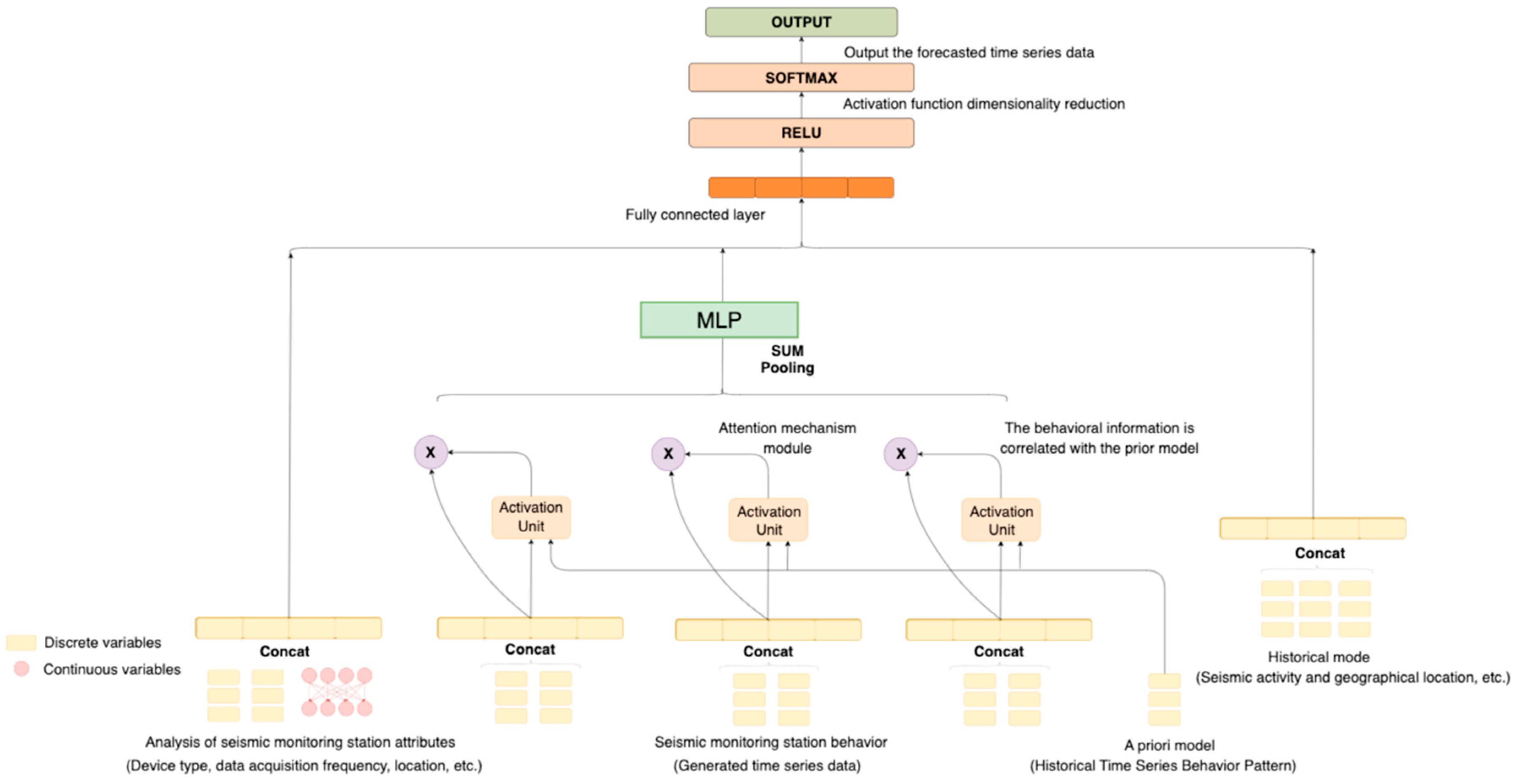
If we only combine the prior knowledge pattern recommendation business with the DIN model, although we can obtain prediction sequences that match the station data features, the level of match with the original data is not high, and the accuracy of the recommendation results is relatively low. To address these issues, this section proposes an improved algorithm that incorporates an MLP neural network. The output of the previous model is used as an intermediate result, which is further processed to optimize the model and improve the accuracy of the recommendations. The final model is illustrated in Figure 5.

The MLP network is used in this study to achieve deep matching between the station behavior and the prior knowledge patterns in the knowledge base. MLP networks are advantageous in capturing nonlinear relationships between vectors and can adjust their network dimensions during the training process, making them more convenient to use. The MLP network itself is a fully connected neural network, where all neurons in each layer are connected to neurons in the next layer with different weights. The structure of the MLP network is illustrated in Figure 6.

The MLP network in this study can be divided into two specific types. The first type of network processes the behavior of all the stations called by the attention mechanism module, enhancing the compatibility between a station and its historical behavior. This set of stations is denoted as $R_u$, with their common behavioral features represented as $B_u$, and the output is the set of similar stations $R_k$. The second type of MLP network aims to aggregate the duplicate sets of stations obtained from the attention mechanism module. It then adjusts the duplicate sets of stations in terms of their number to facilitate the corresponding functional sequence combination. The duplicate sets are denoted as $R_G$, and their specific functional behavioral features are represented as $B_g$. The output of this network is a set of similar stations, $R_s$. The optimization objective is represented by Equations (11) and (12), where $Q_{pub}\left(\right)$ is the mapping function of the training result, and ω represents the parameters in the hidden layer:

$$Q_{pub}(\left(R_u,\omega \right),B_u)$$

(11)

To train the specific features of duplicate stations ($Q_{spe}$()), both MLP networks are trained using forward propagation and backpropagation.

$$Q_{spe}(\left(R_G,\omega \right),B_g)$$

(12)

After the model training is completed, the trained networks are used to process the input source domain station representation set $R_i^S=\{r_1^S,r_2^S,\dots ,r_n^S\}$. As shown in Equations (13) and (14), $x$ represents the input layer vector of the MLP network and y represents the output layer vector. The number of layers in the MLP network is denoted as $N$, and $\beta$ represents the collection of bias parameters in the MLP network:

$$\begin{gathered} x_i=r_i^S, \\ {X}_j=\sigma \left(r_i^S·\beta \right)=f\left(W·x_{j-1}\right)+b_{j(j=2,\dots ,N)} \\ y=f\left(W_N·x_N\right)+b_N \end{gathered}$$

(13)

where $\sigma \left(\right)$ is the activation function of the MLP network. In this paper, we use the tanh function as the activation function in the hidden layer and output layer.

$$\sigma \left(x\right)=\frac{1-e^{-2x}}{1+e^{-2x}}$$

(14)

The trained shared mapping network mlp-pub and specific mapping network mlp-spe are combined to obtain a new representation of the station behavior set. Here, $\beta$ is a weighting factor that can adjust the importance ratio of specific features and shared features in the final station representation.

The trained shared mapping network, mlp-pub and the specific mapping network, mlp-spe, are combined to obtain a new set of station behaviors. The fusion is achieved by incorporating an influence factor, $\beta$, which can adjust the relative importance of specific features and shared features in the final representation of the stations. The process is shown in Formula (15):

$$R=\beta R_{mlp\text{-}pub}+(1-\beta )R_{mlp\text{-}spe}$$

(15)

Then, the matrix multiplication is performed between the stations and the corresponding prediction sequence score matrix, as shown in Equation (16):

$$\widehat{S}=R·S$$

(16)

Finally, the time series that best matches the historical behavior patterns of the station is recommended based on higher recommendation scores.

5. Simulation and Results Evaluation

5.1. Dataset

(1)

Dataset Introduction

To validate the effectiveness of the proposed method, this study selected a test dataset from the priori knowledge base simulating station priori models. It contains the station behavior information and relevant prior model information required for this paper. Using simulated stations for testing not only reduces the workload but also solves the cold start problem. In the experiment, a dataset with a total size of 53 M was chosen, comprising station behavior data and prior model data. Additionally, the station behavior data were collected by simulating the invocation of prior model information by the stations. During this process, a significant number of prior models that did not align with the historical behavior patterns of the stations were filtered out. Only the behavior patterns that effectively and efficiently invoked the prior models were retained for further analysis.

The dataset used in this paper contains two subsets: the station behavior dataset “Stations_data.txt” and the priori model dataset “PrioriModel.txt”. The label style in the station behavior dataset is as follows: StationId|PrioriModel_Id|Time, which includes the station’s ID, the priori model ID it called, and the timestamp of the call. The priori model dataset is primarily used to record basic information about the priori models, with a list style as follows: |PrioriModel_Id|PrioriModel_Type|. The data formats for the two datasets are defined, as shown in Figure 7 and Figure 8. The meanings of each field are as follows:

• StationID: station equipment ID;
• PrioriModel_Id: The called priori model ID, with the letter ‘E’ indicating the model library it belongs to. The model libraries are numbered from A to Q, and the individual models within each library are numbered from 1 to 100;
• Time: time of the station’s priori model invocation;
• PrioriModel_Type: The type of the model, with the numbers in the array, indicates a progressive relationship. For example, in Figure 8, the prior model with ID “E59” and model type represents the historical data pattern–trend prediction.

(2)

Data preprocessing

The data processing workflow mainly consists of two core steps. First, we need to determine the value of the sliding time window N and convert the data from one-dimensional to two-dimensional. In this step, we focus on the data between 4 a.m. and 9 a.m. each day and decide to set the size of the sliding window N to the total number of seconds in this period, that is, 5 h or 18,000 s. This setting strategy is based on the relevance, completeness, and computational feasibility of the data. Since the data within this period exhibit certain cyclical features, setting a 5 h sliding window can ensure that each window contains the complete cycle pattern of the data, thereby providing favorable conditions for the subsequent data analysis.

Next, to enhance the generality of the data, we form a set of positive and negative samples by randomly replacing the time series in the sequence of station calls. Additionally, we randomly extract 20% of the data as a test set, while the remaining data form the training set.

5.2. Evaluation Metrics

In the experiments of this chapter, AUC (area under curve) and LogLoss are used as the primary evaluation metrics. LogLoss has already been introduced in Section 3.4. This section will mainly introduce the AUC evaluation metric. In machine learning, samples are sorted based on the predictions made by the learner on the test set. Each sample is predicted as a positive example in this order, and the true positive rate (TPR) and false positive rate (FPR) are calculated each time. The curve drawn with the TPR on the y-axis and FPR on the x-axis is called the ROC (receiver operating characteristic curve) curve. The AUC is the area enclosed by the ROC curve and the coordinate axis. The larger the AUC, the more reasonable the sorting results of the samples. The definitions of TPR and FPR are shown in Equations (17) and (18):

$$TPR=\frac{TP}{TP+FN}$$

(17)

$$FPR=\frac{FP}{TN+FP}$$

(18)

It is worth noting that the results of Equations (17) and (18) are dimensionless. This allows us to assess the predictive accuracy of the model fairly, without being affected by specific measurement units. Their specific definitions are shown in

Table 1. Classification results from confusion matrix.

True Value	Predicted Value
	Positive Instance	Negative Instance
Positive instance	TP (True Positive)	FN (False Negative)
Negative instance	FP (False Positive)	TN (True Negative)

.

GAUC, also known as the average value of AUC, is calculated using Equation (19):

$$GAUC=\frac{\sum _{R_i}{\lambda }_{R_i}·{AUC}_{R_i}}{\sum {\lambda }_{R_i}}$$

(19)

In the given formula, ${\mathsf{\Sigma }}_{R_i}$ represents the summation over all categories $R_i$, and ${AUC}_{R_i}$ represents the area under the ROC curve (AUC) for category $R_i$. Moreover, ${\lambda }_{R_i}$ denotes the corresponding weight of category $R_i$, with values ranging from 0 to 1. Each ${\lambda }_{R_i}$ is set to a candidate value within the range [0, 0.1, 0.2, …, 0.9, 1]. Then, for each ${\lambda }_{R_i}$ value, the GAUC (generalized area under the ROC curve) is computed, and the ${\lambda }_{R_i}$ value that maximizes the GAUC is selected as the final parameter. Consequently, a larger AUC value indicates a better predictive performance of the model, whereas a smaller LogLoss value indicates a better predictive performance.

5.3. Experiment Platform

The hardware environment for this experiment is as follows:

(1)

Hardware environment:

• Operating system: Windows 10 64-bit (Microsoft, Redmond, MA, USA);
• Processor: Intel(R) Core(TM) i7-11800H CPU @ 2.40GHz (Intel, Santa Clara, CA, USA);
• Memory: 16 GB (Unspecified Manufacturer, Unspecified City, Unspecified Country);
• Graphics card: GeForce RTX3060 (NVIDIA, Santa Clara, CA, USA).

(2)

Software environment:

• Programming language: Python 3.8 (Python Software Foundation, Wilmington, DE, USA);
• Deep learning framework: Tensorflow 2.4.1 (Google LLC., Mountain View, CA, USA).

5.4. Experimental Process and Analysis

(1)

Comparison of experimental results after model improvement

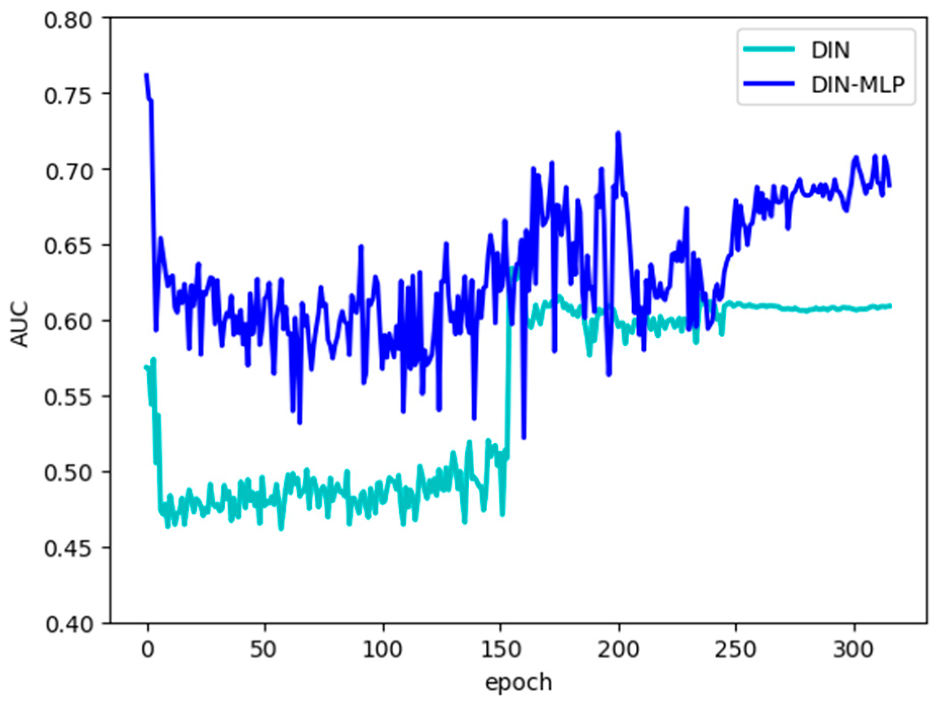
This article compares the performance of the DIN model and the DIN–MLP model, with Figure 9 showing the results obtained by the two models.

From the experimental results curves of the two models, it can be seen that during the first five data iterations, the AUC results are consistently decreasing. Considering that the data used in the current experiment are all collected by individuals from the priori knowledge base, the scale, regularity, and sample type ratio of the data are not as professional as many public datasets, so this situation appears in the early stages of the experiment. From the 50th to the 150th iteration, the DIN model results are basically between 0.45 and 0.5, whereas the DIN–MLP results fluctuate between 0.55 and 0.65, and the results after the improvement are generally better than the original DIN model. From the 150th to the 250th iteration, it can be seen that the experimental results of the improved model fluctuate more, and the results of the original DIN model rise to about 0.6 and even exceed the results after the improvement in some intervals. After 250 times, the results of the two models gradually stabilize. The original DIN model results are stable at around 0.61, and the results of the improved model are stable at around 0.69.

It can be seen that overall, the metric results of DIN–MLP are higher than the original DIN model. Intuitively, the results after the improvement are about 8 percentage points higher than the original ones, achieving a significant improvement. From the data results, it can also be seen that there are different degrees of fluctuation in the calculation process, considering that there are fewer datasets in this experiment, and the randomness in the data collection process is strong. Therefore, the density of the same kind of data is small, and it is difficult to capture the detailed rules in the model calculation process, and the experimental results cannot reach a higher level. Moreover, choosing different numbers of recommendation combinations means that the AUC indicator will change accordingly, so we also need to consider adjusting this parameter’s impact on the accuracy value and the diversity of the predicted sequence combinations;

(2)

Comparison of results under different parameters

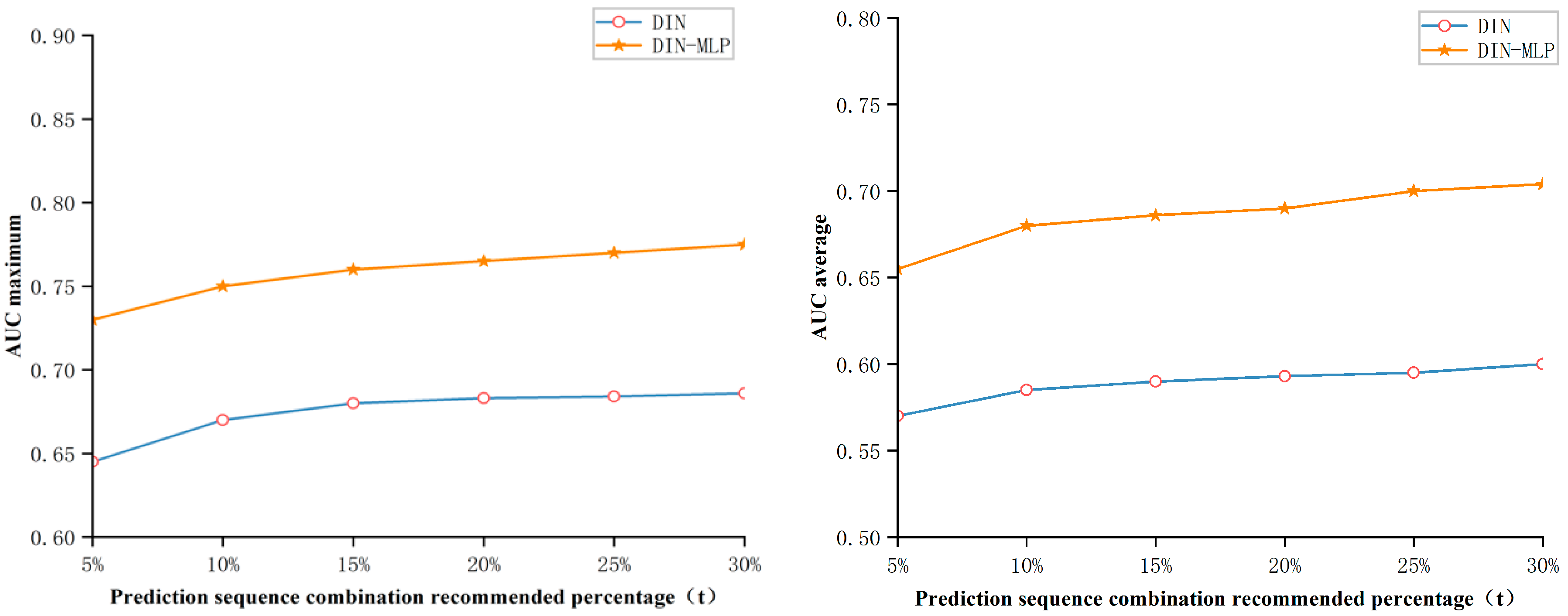
When the priori knowledge base recommends time series combinations for stations, it will produce many recommended results, which require certain trade-offs. To ensure the accuracy of the recommended results, this paper adopts the strategy of keeping the top-t recommended results, i.e., keeping the top t% of the final recommended sequence combination results. If the value of t is relatively small, it will lead to too few recommended sequence combinations obtained by the priori knowledge base, and a lack of diversity will result in a too low fault tolerance, and situations that do not meet the functional requirements of the stations may arise. If the value of t is relatively high, although it can ensure station function requirements and also improve a certain degree of accuracy, it is difficult to guarantee station performance requirements in this case, which may lead to a decrease in work efficiency. Therefore, it is necessary to explore the proportion of the number of predicted sequence combination results to be selected. In this section of the experiment, we first ruled out situations where the selection ratio is too high or too low and selected the range of 5–30%, with the other experimental settings the same as the main experiment. The experimental results are shown in Figure 10:

Firstly, looking at the average accuracy growth trend in Figure 10, when the value of t is greater than 25%, the growth of accuracy becomes more gentle, so the range of values can be reduced to within 25%. And the accuracy grows larger between 5 and 10%, and in combination with Figure 11, it can be stated that within this range the types of recommended sequences will see a substantial increase. However, when the value of t is more than 20%, the speed of increase in sequence combination diversity begins to slow down, indicating that the impact of the increase in t value on sequence combination diversity begins to diminish. But when t is less than 15%, the number of recommended sequence combinations is too few to meet the functional requirements of the stations. Therefore, overall, it is reasonable to set the value of t in the range of 15–20%.

According to the above parameter settings for calculation, the indicator results shown in the following table can be obtained.

As can be seen from

Table 2. Comparison of experimental results.

Model	GAUC	LOSS
DIN–MLP	0.6921	0.4375
DIN	0.5894	0.5016

, if we simply directly link the business, input data, and DIN model, the accuracy is not high. Although these two types of businesses are similar, they cannot be conflated. Firstly, although users and stations belong to one group, user behaviors may not necessarily follow a pattern, whereas stations do exhibit regularity based on their foundational function settings. Therefore, in this paper, an MLP network was added to the attention mechanism module, reinforcing the network’s memory of the regular behaviors of the stations. This led to an 11 percent point increase in the average accuracy of the improved DIN model and a significant improvement in the AUC results. Despite the appearance of instability in the accuracy curve fitting during the training process of DIN–MLP in the previous graphs, overall, the integration of the MLP network has a substantial impact on the DIN model’s results in prior knowledge base pattern recommendations. In addition, through experiments, the value range in the percentage parameter for recommendation results was determined, achieving good results under both the AUC and GAUC evaluation metrics.

6. Conclusions

This paper introduces the improved DIN–MLP model, based on the DIN model. By integrating the prior knowledge base with the DIN model, the prior knowledge base’s recommendation business is implemented, enabling it to recommend time series that align with the data characteristics of seismic monitoring stations for future time steps’ data prediction purposes. However, merely combining the prior knowledge base business with the DIN model makes it challenging to deeply explore the relationship between station behaviors and prior model attributes, leading to a lower prediction accuracy. Thus, improvements have been made to the model. The introduction of the MLP neural network after the attention mechanism module matches the station behavior attributes with similar historical pattern attributes multiple times, further enhancing the accuracy and interpretability of recommendations. This experiment utilizes the AUC and GAUC as evaluation metrics, conducting multiple comparative experiments and summarizing the results. The final experimental results indicate that the DIN–MLP model, compared to the original DIN model, increases prediction accuracy by approximately 11 percentage points. These numerical results visually demonstrate the performance improvement brought about by the model’s enhancement.

In practical applications, the research findings of this paper can be employed for data prediction and recommendation in earthquake monitoring stations, thus enhancing the performance of seismic monitoring systems. Through the improved DIN–MLP model, we have achieved more accurate forecasting of station data characteristics, providing more precise recommendations for time series combinations to earthquake monitoring stations. This holds a significant importance in boosting the efficiency and accuracy of seismic monitoring, offering substantial support to fields such as earthquake early warning and prediction. Considering the substantial variation in hardware configurations and data characteristics among earthquake monitoring stations, disparities in missing data between stations may also exist. By utilizing the data matching mechanism of the priori model, we can tailor exclusive data prediction and completion models for each station based on their unique characteristics and requirements. This personalized approach effectively harnesses the commonalities and differences among stations, thus better addressing the data gaps within stations.

Although this study has achieved certain preliminary results, we are also aware of some limitations. Currently, our main focus has been on using the AUC as the primary evaluation metric to assess the model’s performance; however, it may have its limitations in certain situations. In future research, besides continuing to optimize the model’s performance evaluation, we plan to conduct a more comprehensive evaluation of the DIN–MLP model through both classification and regression tasks, aiming for better improvements and advancements. During this process, we intend to introduce more model comparisons and auxiliary metrics, such as accuracy, recall, RMSE (root mean square error), and MAE (mean absolute error), to comprehensively assess the performance of the DIN–MLP model in both classification and regression tasks. By comparing results across different tasks, we can gain a more comprehensive understanding of the model’s strengths and limitations, leading to more accurate conclusions.

References

- Du, J. Research on Airport Noise Monitoring Data Completion Based on Deep Learning. Master’s Thesis, Nanjing University of Aeronautics and Astronautics, Nanjing, China, 2019. [Google Scholar] [CrossRef]
- Mandelli, S.; Lipari, V.; Bestagini, P.; Tubaro, S. Interpolation and denoising of seismic data using convolutional neural networks. arXiv 2019, arXiv:1901.07927. [Google Scholar] [CrossRef]
- Park, J.; Yoon, D.; Seol, S.J.; Byun, J. Reconstruction of seismic field data with convolutional U-Net considering the optimal training input data. In Proceedings of the SEG International Exposition and Annual Meeting, San Antonio, TX, USA, 15–20 September 2019; SEG: Houston, TX, USA. [Google Scholar] [CrossRef]
- Wang, B.; Zhang, N.; Lu, W.; Wang, J. Deep-learning-based seismic data interpolation: A preliminary result. Geophysics 2019, 84, V11–V20. [Google Scholar] [CrossRef]
- Li, X.; Wu, B.; Zhu, X.; Yang, H. Consecutively Missing Seismic Data Interpolation Based on Coordinate Attention Unet. IEEE Geosci. Remote Sens. Lett. 2022, 19, 3005005. [Google Scholar] [CrossRef]
- Yu, J.; Wu, B. Attention and Hybrid Loss Guided Deep Learning for Consecutively Missing Seismic Data Reconstruction. IEEE Trans. Geosci. Remote Sens. 2022, 60, 5902108. [Google Scholar] [CrossRef]
- Jiang, L.; Dai, B.; Wu, W.; Loy, C.C. Focal Frequency Loss for Image Reconstruction and Synthesis. In Proceedings of the 2021 IEEE/CVF International Conference on Computer Vision (ICCV), Montreal, QC, Canada, 10–17 October 2021; pp. 13899–13909. [Google Scholar] [CrossRef]
- Xu, J.; Huang, Y.; Cheng, M.-M.; Liu, L.; Zhu, F.; Xu, Z.; Shao, L. Noisy-As-Clean: Learning Self-Supervised Denoising from Corrupted Image. IEEE Trans. Image Process. 2020, 29, 9316–9329. [Google Scholar] [CrossRef] [PubMed]
- Fei, X.; Hui, Y.; Wu, B.; Wang, R.; Lian, X. Self-supervised continuous missing seismic data interpolation method. In Proceedings of the 2022 China Petroleum Physical Exploration Academic Annual Conference (Next Volume), Haikou, China, 26–29 April 2022; pp. 502–505. [Google Scholar] [CrossRef]
- Gui, C.; Liu, Y. Unsupervised deep learning seismic data reconstruction based on dropout sampling. In Proceedings of the 2022 China Petroleum Physical Exploration Academic Annual Conference (Next Volume), Haikou, China, 26–29 April 2022; pp. 553–556. [Google Scholar] [CrossRef]
- Meng, H.Y.; Yang, H.C.; Zhang, J.C. An unsupervised residual network approach to seismic data reconstruction. Pet. Geophys. Explor. 2022, 57, 789–799+736–737. [Google Scholar] [CrossRef]
- Huang, Z.; Yu, C.; Ni, J.; Liu, H.; Zeng, C.; Tang, Y. An Efficient Hybrid Recommendation Model with Deep Neural Networks. IEEE Access 2019, 7, 137900–137912. [Google Scholar] [CrossRef]
- Liu, L.; Wang, Z. Research on cold-start problem in user based collaborative filtering algorithm. In Proceedings of the 8th International Conference on Computer Engineering and Networks (CENet2018), Shanghai, China, 17–19 August 2018; Springer International Publishing: Cham, Switzerland, 2020. [Google Scholar] [CrossRef]
- Natarajan, S.; Vairavasundaram, S.; Natarajan, S.; Gandomi, A.H. Resolving data sparsity and cold start problem in collaborative filtering recommender system using linked open data. Expert Syst. Appl. 2020, 149, 113248. [Google Scholar] [CrossRef]
- Ren, J.; Xu, X.; Yu, H. Improved Collaborative Filtering Algorithm Incorporating User Information and Using Differential Privacy. In Proceedings of the Computer Supported Cooperative Work and Social Computing: 14th CCF Conference, Chinese CSCW 2019, Kunming, China, 16–18 August 2019; Revised Selected Papers 14; Springer: Singapore, 2019. [Google Scholar] [CrossRef]
- Adilaksa, Y.; Musdholifah, A. Recommendation System for Elective Courses using Content-based Filtering and Weighted Cosine Similarity. In Proceedings of the 2021 4th International Seminar on Research of Information Technology and Intelligent Systems (ISRITI), Yogyakarta, Indonesia, 16–17 December 2021; pp. 51–55. [Google Scholar] [CrossRef]
- Abbattista, F.; Degemmis, M.; Licchelli, O.; Lops, P.; Semeraro, G.; Zambetta, F. Improving the usability of an e-commerce web site through personalization. Recomm. Pers. Ecommerce 2002, 2, 20–29. [Google Scholar]
- Zhang, S.; Yao, L.; Sun, A.; Tay, Y. Deep learning based recommender system: A survey and new perspectives. ACM Comput. Surv. (CSUR) 2019, 52, 1–38. [Google Scholar] [CrossRef]
- Logesh, R.; Subramaniyaswamy, V. Exploring hybrid recommender systems for personalized travel applications. In Cognitive Informatics and Soft Computing: Proceeding of CISC 2017; Springer: Singapore, 2019. [Google Scholar] [CrossRef]
- Kiran, R.; Kumar, P.; Bhasker, B. DNNRec: A novel deep learning based hybrid recommender system. Expert Syst. Appl. 2020, 144, 113054. [Google Scholar] [CrossRef]
- Khan, Z.; Iltaf, N.; Afzal, H.; Abbas, H. DST-HRS: A topic driven hybrid recommender system based on deep semantics. Comput. Commun. 2020, 156, 156–183. [Google Scholar] [CrossRef]
- Sun, Z.; Zhang, J.; Sun, H.; Zhu, X. Collaborative filtering based recommendation of sampling methods for software defect prediction. Appl. Soft Comput. 2020, 90, 106163. [Google Scholar] [CrossRef]
- Xiong, R.; Wang, J.; Zhang, N.; Ma, Y. Deep hybrid collaborative filtering for web service recommendation. Expert Syst. Appl. 2018, 110, 191–205. [Google Scholar] [CrossRef]
- Covington, P.; Adams, J.; Sargin, E. Deep Neural Networks for YouTube Recommendations. In Proceedings of the Acm Conference on Recommender Systems ACM, Boston, MA, USA, 15–19 September 2016; pp. 191–198. [Google Scholar] [CrossRef]