Abstract
Abnormal electricity consumption behavior not only affects the safety of power supply but also damages the infrastructure of the power system, posing a threat to the secure and stable operation of the grid. Predicting future electricity consumption plays a crucial role in resource management in the energy sector. Analyzing historical electricity consumption data is essential for improving the energy service capabilities of end-users. To forecast user energy consumption, this paper proposes a method that combines adaptive noise-assisted complete ensemble empirical mode decomposition (CEEMDAN) with long short-term memory (LSTM) networks. Firstly, considering the challenge of directly applying prediction models to non-stationary and nonlinear user electricity consumption data, the adaptive noise-assisted complete ensemble empirical mode decomposition algorithm is used to decompose the signal into trend components, periodic components, and random components. Then, based on the CEEMDAN decomposition, an LSTM prediction sub-model is constructed to forecast the overall electricity consumption by using an overlaying approach. Finally, through multiple comparative experiments, the effectiveness of the CEEMDAN-LSTM method is demonstrated, showing its ability to explore hidden temporal relationships and achieve smaller prediction errors.
1. Introduction
With the rapid development of science, technology, and the economy, the demand for electricity continues to increase, leading to the expansion of the power grid and the increasing complexity of power systems. The issue of data security in power grids has also attracted attention, as ensuring the secure and reliable operation of the power system is crucial for the stable functioning of the national economy.
Numerous research studies and discussions have been conducted internationally on smart grids. As a key technology in smart grids, the advanced metering infrastructure integrates smart meters, communication networks, and data management systems, enabling bidirectional communication between utility centers and customers [1]. The application of digital smart meters and the introduction of network layers in metering systems have also introduced new avenues for electricity theft [2]. Electricity theft not only causes financial losses for power companies but also poses a significant risk to the security of the power grid. It can lead to damage to low-voltage electrical equipment, local power supply interruptions, and even power grid accidents. In the event of a cascading effect, it can result in severe consequences such as large-scale power outages. Additionally, electricity theft incidents have resulted in electrical fires and casualties. In recent years, nearly 40% of electrical fires have been caused by abnormal electricity consumption and illegal acts of damaging power facilities, with even higher proportions in densely populated areas such as shared rental accommodations. Once electricity thieves succeed, they often excessively use high-energy-consuming appliances, leading to line overloads and serious fire safety hazards. Non-technical losses in power systems represent an urgent safety issue. Predicting user electricity consumption has significant guidance for power companies in handling related matters. Furthermore, the focus of prediction has shifted from a macroscopic perspective to a microscopic perspective, emphasizing the importance of load prediction in improving end-user energy service capabilities.
In the context of the major domains of “New Infrastructure”, including 5G base stations, big data centers, artificial intelligence, and industrial Internet, the emphasis lies in the era of digitization and intelligence. The Internet of Things (IoT) provides robust data support for rational data utilization [3]. Proper utilization of electric grid data enables the monitoring and detection of grid conditions, ensuring real-time system security [4,5]. By mining historical and real-time data [6], the diagnosis, optimization, and prediction of grid states can be achieved, thereby enhancing grid management capabilities, optimizing resource allocation, identifying operational patterns, and formulating rational plans to ensure grid stability, security, and economic efficiency. Statistical data indicates that with every 10% increase in the utilization of power data, the profitability of power companies can rise by 20–40%. However, the challenge lies in the effective extraction of valuable information from the vast and heterogeneous power data [7], including identifying abnormal users and predicting short-term power loads for the future. A comparison between previous research and this study is shown in Table 1.

Table 1.
The comparison of related works. (“√” if the solution satisfies the property, “×” if not).
This paper proposes a user electricity consumption prediction method that combines CEEMDAN with LSTM networks in the context of secure electricity usage. The contributions of this study can be summarized as follows:
- By enhancing the algorithm, the utilization of CEEMDAN effectively characterizes the local transient characteristics of the signal. This greatly assists the load prediction model in exploring hidden temporal relationships more comprehensively.
- Based on the CEEMDAN algorithm, a specially designed sliding window is employed to avoid the inefficiency of model training caused by excessively long input data sequences. The sliding window preserves the long-term trend components, periodic components, and random components of the load.
- Leveraging the capabilities of LSTM, a multi-layer neural network is used to individually model and predict the components and residuals. This approach better captures the dynamic patterns and random fluctuations of electricity consumption data, thereby enhancing the accuracy and interpretability of electricity load prediction. The predicted results of these components are then reconstructed to obtain the final electricity consumption prediction.
2. Related Works
With the advancement of technology, the analysis and prediction of anomalies in various industries such as weather [11], transportation [12,13,14], and electricity [15] have been conducted to avoid losses. Particularly, the demand for electrical energy continues to grow. The safety issues in the power industry have attracted widespread attention. Currently, methods for electricity consumption forecasting can be mainly classified into two categories: the first category includes traditional forecasting methods such as linear regression analysis, traditional time series modeling, and periodic factor models; the second category includes machine learning prediction methods, such as time series methods [16], deep learning networks [17,18], gradient boosting decision trees, and support vector machine regression [19].
For the detection and prediction of electricity consumption, transmitting a large amount of data from different regions to a central node for detection and prediction not only suffers from poor real-time performance but also increases unnecessary energy consumption [20]. Edge computing has been widely studied in various industries, enabling data processing at the edge [21,22], thereby improving data processing efficiency and avoiding security issues associated with data transmission. Ning et al. [23] developed a cost-effective home health monitoring system based on mobile edge computing and 5G technology, reducing the cost of IoT healthcare systems. As the demand for real-time mobile application processing continues to grow, multi-access edge computing has been considered a promising paradigm to extend computational resources to the network edge [24,25,26]. In the context of edge computing, Wang et al. [27] also proposed wireless charging methods to address the insufficient energy consumption of mobile edge computing.
High-precision electricity forecasting plays a crucial role in maintaining a balanced power supply, and deep learning has proven beneficial in electricity load prediction, yielding promising results in various practical applications [28]. Significant advancements have been made in deep learning for time series forecasting [29]. Recurrent neural networks (RNNs) have achieved remarkable success in natural language processing [30], semantic recognition [31], and image recognition [32], making them a commonly used network framework for time series prediction. However, in the field of electricity load forecasting, where extensive time series data extraction and analysis are required, the gradient vanishing problem of RNNs has emerged as a major obstacle limiting their predictive performance [33,34]. In response to this limitation, LSTM, which is built upon the developments of RNNs, has effectively addressed the gradient vanishing problem and has become the main direction of current research [35].
Lin et al. [36] validated the suitability of LSTM-based models for residential load forecasting, indicating further improvements when more data are available. Kong et al. [8] proposed an LSTM-based forecasting model for short-term load prediction in industrial and commercial enterprises, considering various factors such as dates. Through empirical experiments, they demonstrated its excellent performance across multiple metrics. However, directly applying prediction models to non-stationary short-term power consumption data hinders the exploration of deeper temporal features [37]. Moreover, with the majority of vehicles being electric, the temporal feature problem becomes more complex [38,39,40]. Saman et al. [41] presented a combined algorithm that integrates empirical mode decomposition (EMD) with LSTM neural networks for short-term load forecasting. Their approach effectively improved prediction accuracy while highlighting the advantages of signal decomposition in load forecasting. Nevertheless, EMD algorithms are prone to mode mixing, which can lead to a loss of specific physical meanings in the intrinsic mode functions (IMFs) [42]. Chen et al. [43] proposed a model based on deep residual networks to predict short-term load, devising an improved deep residual network to enhance the prediction results. They employed a two-stage ensemble strategy to enhance the generalization capability of the proposed model. Although the aforementioned studies have explored short-term electricity forecasting techniques from various aspects, there is still room for improving the accuracy of non-stationary short-term user electricity predictions, warranting further research. To overcome the limitations of analysis methods lacking adaptability, Norden proposed a signal time-frequency processing approach using EMD and Hilbert spectral analysis. Due to its adaptive nature, this decomposition method is suitable for analyzing and processing nonlinear and non-stationary signals. The decomposition is performed based on the inherent time scale characteristics of the data, eliminating the need for pre-defined basis functions. It is precisely due to this adaptive characteristic that, in theory, the EMD method can be applied to any type of signal decomposition. Therefore, when dealing with non-stationary and nonlinear data, EMD exhibits significant advantages.
3. Sequence Decomposition Based on Sliding Window
This study aims to compare various sequence decomposition methods to identify the most suitable method for load data decomposition. Additionally, a special sliding window is designed to extract the periodic component, trend component, and random component of the load sequence.
3.1. Empirical Mode Decomposition
Once introduced, the EMD method quickly found applications in various engineering fields, such as wind power, solar energy, atmospheric observations, and brain signals, for mode parameter recognition and identification. The EMD method iteratively extracts a series of IMFs and applies the Hilbert transform to obtain physically meaningful instantaneous frequencies for each component. Compared to traditional signal analysis methods, the EMD method is not constrained by the uncertainty principle and can achieve higher frequency resolution. Moreover, the EMD decomposition is based on the intrinsic characteristics of the signal itself, eliminating the need for predefined basis functions, which gives it an unparalleled advantage in terms of adaptability. The EMD method enables adaptive decomposition and processing of non-stationary signals.
Due to its reliance on the intrinsic characteristics of the signal, the EMD approach possesses complete adaptability. The EMD decomposition method assumes a hidden underlying condition that for any given sequence, there exist numerous oscillatory modes with different frequencies that superpose to form the entire data. Each oscillatory mode, defined as an IMF, must satisfy the following two conditions:
- 1.
- At any given time point, the average value of the envelope defined by the maximum and minimum values is zero.
- 2.
- Over the entire dataset, the number of extrema is either equal to the number of zero-crossings or, at most, differs by one.
The steps for EMD decomposition are as follows:
- 1.
- For any signal sequence , first identify all the extrema points on . Then, use cubic spline interpolation to connect all the local maxima to form the upper envelope. Similarly, connect all the local minima to form the lower envelope, ensuring that all data points lie between these two envelopes. The average value of the upper and lower envelopes is denoted as . Calculate the difference between and , denoted as , using the following equation:
- 2.
- Replace the original sequence with and repeat step (1) until satisfies the two conditions of an IMF. that satisfies these conditions is considered as the first IMF. The standard deviation (SD) is commonly used to determine whether qualifies as an IMF.where T represents the length of sequence . denotes the data after k iterations of sifting. It is generally recommended to set the SD value between 0.1 and 0.3. When the condition is met, the decomposition stops, and the first IMF component is obtained.
- 3.
- Subtracting component from the original sequence yields the residual component , i.e.:A flowchart of the EMD algorithm is illustrated in Figure 1:
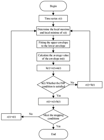 Figure 1. Flowchart of the EMD Algorithm.
The process continues by considering as a new sequence and repeating steps (1) and (2) to obtain the second IMF component , and this process is iterated until the termination condition for signal decomposition is met, which is when the residual component becomes a monotonic function. At this stage, is referred to as the residual component of the original sequence. The complete decomposition process and its results are illustrated as follows:
3.2. Ensemble Empirical Mode Decomposition
EMD decomposition is an empirical algorithm without strict mathematical specifications. It has several limitations and drawbacks in practical applications, including mode mixing, spurious components, and endpoint effects. Mode mixing refers to the phenomenon where IMF components from different time scales are mistakenly identified as the same IMF component, or IMF components from the same time scale are decomposed into multiple IMF components. Mathematically, this corresponds to the coupling between different IMF components. Mode mixing affects all IMF components and can lead to the presence of physically meaningless IMF components as the iteration progresses. To address this issue, a new improved algorithm called EEMD is introduced. The EEMD algorithm follows the following steps:
- 1.
- A Gaussian white noise sequence , N is added to the original signal , creating a mixed signal of signal and noise: Bulleted lists look like this:
- 2.
- Perform EMD decomposition on the signal with added noise, resulting in IMF components and a residual component , as follows:
- 3.
- Repeat step (2) to obtain sets of distinct IMF component collections and residual collections.
The final result is obtained by performing ensemble averaging on the N sets of distinct IMF component collections and residual collections. The IMF components corresponding to the original signal can be represented as follows:
To overcome the computational time and residual noise issues associated with EEMD and to reduce the number of sifting iterations with fewer averaging runs, an improved method called CEEMDAN is used. In CEEMDAN, adaptive white noise is added multiple times at each stage to achieve nearly 0% reconstruction error with fewer averaging runs. In this paper, we will analyze and describe the specific application steps of CEEMDAN. Compared to EMD and EEMD methods, CEEMDAN has the following advantages:
- 1.
- Introducing additional noise coefficients to control the noise level during each decomposition [44];
- 2.
- Complete and noise-free reconstruction process [44];
- 3.
- Requires fewer experimental runs and is more efficient [45].
3.3. Sliding-Window-Based CEEMDAN Decomposition for Time Series Analysis
The user’s load profile is a time series that exhibits both periodicity and a certain degree of randomness. The load data are observed at different time scales, such as hours, days, weeks, months, and years, capturing the regularities of residential activities that are nested within larger cycles. Additionally, user behavior contains certain random elements. These characteristics pose challenges to load forecasting. Inspired by signal decomposition techniques, this study utilizes the adaptive CEEMDAN method to decompose the electricity load sequence into its trend, periodic, and random components. This approach, which characterizes the features of the load sequence, provides valuable insights into subsequent forecasting tasks.
CEEMDAN obtains the IMF by introducing white noise with specific frequency bands at each decomposition stage. Firstly, let represent the IMF mode generated by EMD decomposition, represent the white noise that satisfies the standard normal distribution, represent the original signal, and represent the IMF mode generated by CEEMDAN. The specific algorithm is as follows:
Step 1: CEEMDAN conducts I experiments on the original data by adding white noise following a standard normal distribution. The first IMF mode component obtained through EMD decomposition is:
Step 2: In the first stage of , remove the mode component from the original signal and calculate the residual signal:
Step 3: Construct the ensemble residual signal and perform EMD decomposition on the ensemble signal to obtain :
For , the calculation process is similar. First, calculate the k residual signal ; then, calculate the k + 1 IMF component :
Step 4: When the number of extreme points in the residual signal is less than 3, the obtained residual signal cannot be further decomposed, and the algorithm terminates. At this point, a total of K IMF components is obtained, and the final decomposition result is:
In the CEEMDAN method, the coefficient allows for the selection of the signal-to-noise ratio during the noise addition stage. Regarding the amplitude of the added noise in the CEEMDAN method, it follows the EEMD approach, where small-amplitude noise is used to handle signals dominated by high-frequency components, while large-amplitude noise is used to handle signals dominated by low-frequency components. If the amplitude of the added noise is too small or too large, it may lead to suboptimal decomposition results that fail to reflect the periodicity, trend, and other characteristics present in the electricity data.
In order to extract the periodic, trend, and random components from the sequence, a special sliding window is designed in this study for time series segmentation. If the window size is directly determined based on the length of the input sequence for the neural network, it may result in difficulties in separating the trend and periodic components. Therefore, while segmenting the sequence with the sliding window, the purpose of sequence decomposition must be considered: to decompose the trend, periodic, and random components of the sequence. Thus, it is necessary to design a sufficiently large window to encompass the periodic and trend components of the load sequence and then perform decomposition on it. To facilitate efficient model training, fixed-length component data are selectively extracted from the posterior of the window. This process is illustrated in Figure 2.
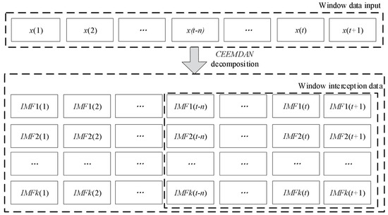
Figure 2.
Windowed CEEMDAN decomposition and IMF component extraction.
4. Design of LSTM Network for Time Series Analysis
To address the issues of gradient vanishing in RNN and overfitting in neural network models during the training process, a power load prediction model based on LSTM and CEEMDAN is proposed, taking into account the periodic, trend, and random components in the electric load time series. This section primarily focuses on the overall network design and some technical details.
4.1. Batch Normalization of Training Samples
During the training of LSTM, mini-batch gradient descent is commonly used as the optimization algorithm. To ensure that each batch input in the hidden layers of the neural network remains in the same distribution, batch normalization (BN) is often employed to preprocess the data. This technique performs both proportional scaling and shifting of the data. Let us assume a batch of samples denoted as , and the principles of BN are described in Equations (16)–(19). The structure of BN is illustrated in Figure 3. The inclusion of the BN layer ensures that each mini-batch sample has the same distribution, preventing the network from being biased toward fitting specific types of samples. When combining the same sample with different samples to form a mini-batch sample set, their outputs will differ. This operation can be understood as data augmentation, and thus, the addition of BN partially addresses the overfitting problem. Laurent et al. [46] introduced BN into the RNN model, which consisted of a five-layer LSTM network. The experimental results indicated that vertical BN improved the convergence speed of the parameters, but horizontal BN did not achieve the intended purpose. Similarly, for RNN, Faraji et al. [47] also found that horizontal BN had poor performance. Additionally, when the network had fewer layers, vertical BN did not produce the expected results and could lead to overfitting. Recent research results suggest that the poor performance of horizontal BN is due to improper scaling parameter settings, resulting in inefficient information propagation. However, in this chapter’s context, considering the small scale of the electricity consumption data, adding a BN layer before LSTM and adjusting the scaling parameter did not yield satisfactory results. Therefore, in the simulation process of this paper, the BN layer was placed after the LSTM layer.
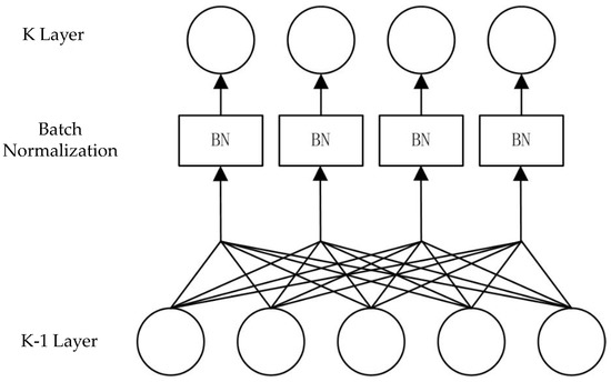
Figure 3.
Batch Normalization.
If BN is applied in the K-1 layer, where represents the mean of the inputs to the K layer unit for a batch of samples, represents the variance of the inputs to the K layer unit for the same batch of samples, and represents the normalized inputs, the model then performs a proportional scaling and shifting operation to output . The scaling factor and the offset, which are required for the transformation, are parameters that need to be learned during model training.
4.2. Overfitting Mitigation with Dropout
There are many solutions currently applied to address the issue of overfitting in neural network models, among which Dropout is a typical approach.
There are several reasons that can lead to overfitting, such as insufficient training data, an excessive number of parameters, and excessive model complexity. In such cases, overfitting of the model can result in high accuracy on the training set but poor performance on the test set. To address this, various measures are commonly taken during neural network training to mitigate overfitting. Dropout, as a commonly used technique for preventing overfitting in neural networks, can effectively alleviate overfitting, improve the model’s generalization ability, and significantly enhance its predictive power in practical applications.
Regularization is a common method used to prevent overfitting, typically achieved by adding a regularization term to the cost function. On the other hand, Dropout directly addresses overfitting by randomly deactivating certain neurons’ information flow during training. As shown in Figure 4, during model training, Dropout randomly cuts off connections between neurons at a certain proportion, causing those neurons to not update their weight matrices for that particular training iteration. In theory, Dropout not only achieves regularization effects but also simplifies the training model. However, in practice, training complexity increases because, with the introduction of Dropout, weight matrix updates become stochastic, leading to a doubling of training time [48].
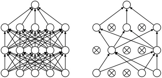
Figure 4.
Comparison between a Standard Neural Network (left) and a Dropout Neural Network (right).
4.3. Design of LSTM Network Model
The user load prediction model based on the LSTM network is shown in Figure 5. The first layer of the entire network consists of LSTM units, where the output at the last time step is utilized as a feature. This is because the output at the last time step can capture the information from the entire time series and integrate it. Subsequently, BN and Dropout are applied to alleviate the issue of overfitting. Finally, three fully connected layers are used to enhance the learning capacity of the network and obtain the prediction results.
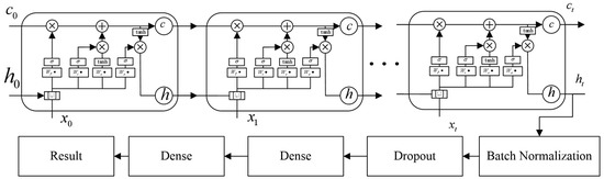
Figure 5.
Model architecture of the LSTM-based user load prediction.
Each LSTM network in the model is responsible for predicting the IMF components and residual components obtained from CEEMDAN decomposition. Therefore, these networks can be executed in parallel.
5. Experimental Design and Result Analysis
To validate the effectiveness of the proposed model, this section conducts two sets of experiments: sequence decomposition experiments in Section 5.1 and model prediction comparison experiments in Section 5.2. The sequence decomposition experiments, based on the actual measured data from smart meters in Ireland, analyze the reasons for using sequence decomposition from an experimental perspective. The model prediction comparison experiments compare the CEEMDAN-LSTM prediction model (experimental group) with the RNN, LSTM, and EMD-LSTM prediction models (comparison group). The stability of different prediction models is evaluated using Root Mean Square Error (RMSE), while the accuracy of the models is assessed by Mean Absolute Error (MAE), reflecting the actual prediction errors of each model.
5.1. Experimental Analysis of Sequence Decomposition
To validate the generalization and diversity of the model, data from 50 randomly selected users were used in the experiment. The first step of the experiment involved decomposing the electricity consumption time series using CEEMDAN. The white noise was added with an amplitude of 0.1 times the standard deviation of the original data, and a total of 200 sets of white noise was added in CEEMDAN.
To avoid complexity in training due to excessively long input data, a sliding window segmentation approach was adopted in this chapter. In order to decompose low-frequency trend components, the sliding window should be set to a relatively large size. The specific configuration is as follows:
- The sliding window encompasses a 60-day data period, and the window is moved by a uniform step size of 1;
- After applying the decomposition to the data within each sliding window, the IMF components are extracted by selectively capturing a fixed-length segment from the rear end of the window.
To address the issue of endpoint effects in the algorithm, this study employs the method of linearly extending the extreme points to handle the endpoints. Additionally, in order to prevent the generation of an excessive number of IMF components, which could lead to increased complexity in later training, the number of IMF components is set to 8.
Figure 6 illustrates the hourly load profile of a specific user, while Figure 7 depicts the decomposition of the user’s hourly load profile. The vertical axis is measured in kW·h, and the horizontal axis represents the sampling points with a sampling interval of 1 h. From Figure 7 it can be observed that the original user’s load time series can be decomposed into eight IMF components (IMF1-IMF8) and one residual component (RES). IMF1-IMF3 exhibit high-frequency components without apparent regular patterns, representing the stochastic components of the load sequence. IMF4-IMF7 exhibit significant periodicity, indicating the periodic components of the original load. IMF8 and RES exhibit prominent trend characteristics, representing the trend components of the load. From the perspective of load characteristics, the load at any given moment can be composed of stochastic, periodic, and trend components. By decomposing a load sequence using CEEMDAN technique, we obtain sub-sequences representing periodicity, trend, and randomness. In a sense, this decomposition precisely corresponds to the characterization of load properties.
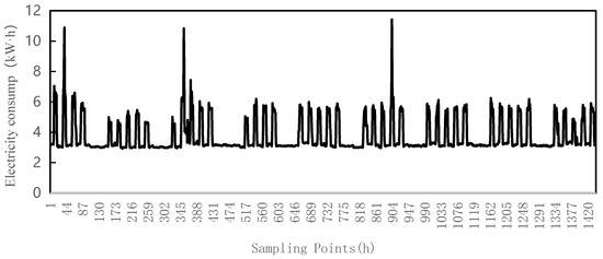
Figure 6.
Hourly raw load profile of a specific user.
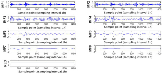
Figure 7.
Hourly raw load CEEMDAN decomposition of a specific user.
5.2. Experimental Evaluation of Model Prediction
To cater to different requirements, separate experiments were conducted for hourly load and daily load prediction. For predicting the electricity consumption for the next hour, the raw data were sampled at hourly intervals. Similarly, for predicting the electricity consumption for the next day, the raw data were sampled at daily intervals. In this experiment, a consistent approach was employed, utilizing 48 historical IMF component values to forecast the IMF component values for the subsequent time period. The data extraction and decomposition were performed using a sliding window technique. To effectively extract the low-frequency trend components, the sliding window was set to a relatively large size.
Due to the increased general applicability of the model, the electricity consumption data from 50 users was utilized. The sliding window included a span of 60 days of data, with a uniform step size of 1. The training dataset, sampled at a daily interval, consisted of 500 days of data. For the training set, the sliding window encompassed 180 days of data with a step size of 1. After decomposition into IMF components, the data points at the end of the window were extracted as a sequence. These data sequences were used for training, while the data from the last 30 days were reserved as the test set.
The input configuration of the LSTM network is shown in Table 2. Longer input lengths of historical data lead to more complexity in model training. This can significantly decrease the speed of model training and even result in optimization difficulties. In comparison to other models, the weight sharing mechanism of LSTM ensures that the number of weights remains independent of the input length. Additionally, the training process of backpropagation exhibits a linear growth relationship between training time and parameter increase. However, to enhance the efficiency of model training and facilitate comparative experiments, this study uniformly adopts 48 historical IMF component values to predict the next IMF component value.
Table 2.
LSTM input settings.
The model is constructed on the Keras platform and utilizes the CuDNNLSTM method for optimizing LSTM training. The parameter configuration of the prediction model is illustrated in Figure 8. Since the experiments uniformly employ the historical values of the previous 48 time intervals to predict the value of the next time interval, the LSTM layer is unfolded for 48 time steps, and the output vector size of the LSTM is set to 81. Both the BN layer and Dropout layer consist of 81 neurons. The Dense layer is composed of 3 layers, with the respective number of neurons being 27, 8, and 1. The final output represents the predicted IMF value for the next time interval. The batch size is set to 30, the learning rate is 0.005, and the dropout probability is 0.5.
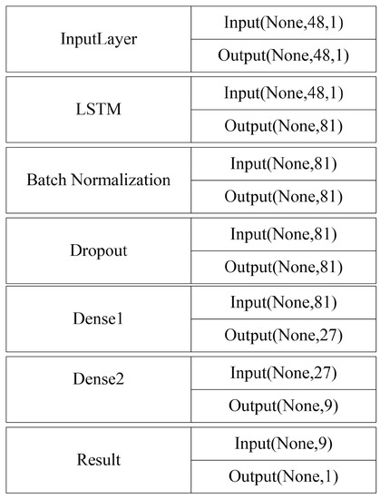
Figure 8.
Visualization of model parameters.
To meet different requirements, the model predicts both hourly load and daily load. In addition, it is compared with the current mainstream methods, including LSTM [8], EMD-LSTM [9], and RNN [10]. Furthermore, the RMSE and MAE of the 50 users are statistically analyzed. Figure 9 and Figure 10 depict the hourly load and daily load prediction results for the four models of a specific user. To provide a more accurate evaluation of the models, this chapter adopts the evaluation metrics of RMSE and MAE, which are classical indicators for load forecasting. The formulas for calculating these two metrics are as follows:
where, n represents the total number of samples, represents the predicted value of the test sample, and represents the actual value of the test sample. The specific prediction errors are shown in Table 3 and Table 4:
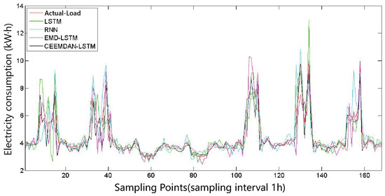
Figure 9.
Hourly specific load prediction.
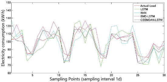
Figure 10.
Daily load prediction for a specific user.
Table 3.
Prediction errors of four models for hourly load of fifty users.
Table 4.
Prediction errors of four models for daily load of fifty users.
From Table 3 and Table 4, it can be observed that the CEEMDAN-LSTM model outperforms the LSTM, EMD-LSTM, and RNN prediction models in terms of both RMSE and MAE metrics. The errors, whether measured by RMSE or MAE, are significantly smaller, indicating that CEEMDAN decomposition does not lose the essential information of the original sequence but rather distributes it among several relatively stable components. The experiments demonstrate that the proposed CEEMDAN-LSTM model decomposes the original data into multiple components with strong periodicity and clear trends. These components can reflect the trend and periodic variations in user load, resulting in more prominent prediction performance compared to a simple LSTM network. Overall, the proposed method is effective and exhibits significantly lower prediction errors compared to other comparative methods.
6. Conclusions
With the increasing popularity of information technology, leveraging data from the power grid to enhance the prediction of abnormal electricity consumption not only improves the theft prediction capability of smart grids but also maintains the security and stability of sub-grids. This paper analyzes the main methods currently applied in this field along with their advantages and disadvantages, and proposes a prediction method based on the combination of CEEMDAN and LSTM. CEEMDAN accurately characterizes the instantaneous frequency features of different frequency components in the signal, allowing it to adaptively represent the local transient characteristics of the signal and greatly assist the load prediction model in exploring hidden temporal relationships. Additionally, a multi-layer LSTM network is designed to independently predict different frequency component parts, and the predicted results of the component data are reconstructed to obtain the final electricity consumption prediction. This paper extensively investigates and designs various aspects, including algorithmic requirements, data preprocessing, feature extraction, model design and optimization, and model testing. Through experimental validation, this prediction method proves to be suitable for nonlinear and non-stationary electricity load forecasting. Through experimental verification, the proposed prediction method exhibits a reduction in errors by 21%, 30%, and 13% compared to LSTM, RNN, and EMD-LSTM prediction methods, respectively. This makes it a suitable forecasting approach for non-linear and non-stationary electric load prediction.
In future work, we will enhance the accuracy of anomaly detection by introducing artificially generated deceptive behaviors into the data. Additionally, we will incorporate other variables into the experiments to reduce experimental errors.
Author Contributions
Conceptualization, H.L. and X.X.; methodology, H.L., X.X. and B.Y.; software, H.L., X.X. and Z.C.; validation, X.X., K.S. and A.T.; formal analysis, H.L. and Z.C.; investigation, H.L., X.X. and B.Y.; resources, H.L. and X.X.; data curation, H.L., K.S. and A.T.; writing—original draft preparation, H.L.; writing—review and editing, X.X.; visualization, Z.C. and K.S.; supervision, H.L., X.X. and A.T.; project administration, H.L. and X.X.; funding acquisition, A.T. All authors have read and agreed to the published version of this manuscript.
Funding
This research was funded by the Researchers Supporting Project number (RSPD2023R681), King Saud University, Riyadh, Saudi Arabia.
Data Availability Statement
Not applicable.
Conflicts of Interest
The authors declare no conflict of interest.
References
- Alavikia, Z.; Shabro, M. A comprehensive layered approach for implementing internet of things-enabled smart grid: A survey. Digit. Commun. Netw. 2022, 8, 388–410. [Google Scholar] [CrossRef]
- Ning, Z.; Sun, S.; Wang, X.; Guo, L.; Wang, G.; Gao, X.; Ykkwok, R. Intelligent resource allocation in mobile blockchain for privacy and security transactions:a deep reinforcement learning based approach. Sci. China Inf. Sci. 2021, 64, 16. [Google Scholar] [CrossRef]
- Kong, X.; Chen, Q.; Hou, M.; Rahim, A.; Ma, K.; Xia, F. RMGen: A Tri-Layer Vehicular Trajectory Data Generation Model Exploring Urban Region Division and Mobility Pattern. IEEE Trans. Veh. Technol. 2022, 71, 9225–9238. [Google Scholar] [CrossRef]
- Gai, N.; Xue, K.; Zhu, B.; Yang, J.; Liu, J.; He, D. An efficient data aggregation scheme with local differential privacy in smart grid. Digit. Commun. Netw. 2022, 8, 333–342. [Google Scholar] [CrossRef]
- Qiao, L.; Dang, S.; Shihada, B.; Alouini, M.S.; Nowak, R.; Lv, Z. Can blockchain link the future? Digit. Commun. Netw. 2022, 8, 687–694. [Google Scholar] [CrossRef]
- Wang, X.; Ning, Z.; Guo, L.; Guo, S.; Gao, X.; Wang, G. Mean-Field Learning for Edge Computing in Mobile Blockchain Networks. IEEE Trans. Mob. Comput. 2022, 1–17. [Google Scholar] [CrossRef]
- Ning, Z.; Chen, H.; Ngai, E.C.H.; Wang, X.; Guo, L.; Liu, J. Lightweight Imitation Learning for Real-Time Cooperative Service Migration. IEEE Trans. Mob. Comput. 2023, 1–18. [Google Scholar] [CrossRef]
- Kong, W.; Dong, Z.Y.; Jia, Y.; Hill, D.J.; Xu, Y.; Zhang, Y. Short-Term Residential Load Forecasting Based on LSTM Recurrent Neural Network. IEEE Trans. Smart Grid 2019, 10, 841–851. [Google Scholar] [CrossRef]
- Wang, Q.; Zhang, Y.; Chen, G.; Chen, Z.; Hee, H.I. Assessment of Heart Rate and Respiratory Rate for Perioperative Infants Based on ELC Model. IEEE Sens. J. 2021, 21, 13685–13694. [Google Scholar] [CrossRef]
- Xia, M.; Shao, H.; Ma, X.; de Silva, C.W. A Stacked GRU-RNN-Based Approach for Predicting Renewable Energy and Electricity Load for Smart Grid Operation. IEEE Trans. Ind. Inform. 2021, 17, 7050–7059. [Google Scholar] [CrossRef]
- Catalina, A.; Alaíz, C.M.; Dorronsoro, J.R. Combining Numerical Weather Predictions and Satellite Data for PV Energy Nowcasting. IEEE Trans. Sustain. Energy 2020, 11, 1930–1937. [Google Scholar] [CrossRef]
- Ning, Z.; Sun, S.; Wang, X.; Guo, L.; Guo, S.; Hu, X.; Hu, B.; Kwok, R.Y.K. Blockchain-Enabled Intelligent Transportation Systems: A Distributed Crowdsensing Framework. IEEE Trans. Mob. Comput. 2022, 21, 4201–4217. [Google Scholar] [CrossRef]
- Ning, Z.; Zhang, K.; Wang, X.; Obaidat, M.S.; Guo, L.; Hu, X.; Hu, B.; Guo, Y.; Sadoun, B.; Kwok, R.Y.K. Joint Computing and Caching in 5G-Envisioned Internet of Vehicles: A Deep Reinforcement Learning-Based Traffic Control System. IEEE Trans. Intell. Transp. Syst. 2021, 22, 5201–5212. [Google Scholar] [CrossRef]
- Wang, X.; Zhu, H.; Ning, Z.; Guo, L.; Zhang, Y. Blockchain Intelligence for Internet of Vehicles: Challenges and Solutions. IEEE Commun. Surv. Tutor. 2023, 11, 27–36. [Google Scholar]
- Raza, M.Q.; Mithulananthan, N.; Li, J.; Lee, K.Y. Multivariate Ensemble Forecast Framework for Demand Prediction of Anomalous Days. IEEE Trans. Sustain. Energy 2020, 11, 27–36. [Google Scholar] [CrossRef]
- González, J.P.; Muñoz San Roque, A.M.S.; Pérez, E.A. Forecasting Functional Time Series with a New Hilbertian ARMAX Model: Application to Electricity Price Forecasting. IEEE Trans. Power Syst. 2018, 33, 545–556. [Google Scholar] [CrossRef]
- Xia, X.; Lin, J.; Jia, Q.; Wang, X.; Ma, C.; Cui, J.; Liang, W. ETD-ConvLSTM: A Deep Learning Approach for Electricity Theft Detection in Smart Grids. IEEE Trans. Inf. Forensics Secur. 2023, 18, 2553–2568. [Google Scholar] [CrossRef]
- Kong, X.; Duan, G.; Hou, M.; Shen, G.; Wang, H.; Yan, X.; Collotta, M. Deep Reinforcement Learning-Based Energy-Efficient Edge Computing for Internet of Vehicles. IEEE Trans. Ind. Inform. 2022, 18, 6308–6316. [Google Scholar] [CrossRef]
- Zhang, G.; Guo, J. A Novel Method for Hourly Electricity Demand Forecasting. IEEE Trans. Power Syst. 2020, 35, 1351–1363. [Google Scholar] [CrossRef]
- Ning, Z.; Dong, P.; Kong, X.; Xia, F. A Cooperative Partial Computation Offloading Scheme for Mobile Edge Computing Enabled Internet of Things. IEEE Internet Things J. 2019, 6, 4804–4814. [Google Scholar] [CrossRef]
- Kong, X.; Wu, Y.; Wang, H.; Xia, F. Edge Computing for Internet of Everything: A Survey. IEEE Internet Things J. 2022, 9, 23472–23485. [Google Scholar] [CrossRef]
- Ning, Z.; Huang, J.; Wang, X. Vehicular Fog Computing: Enabling Real-Time Traffic Management for Smart Cities. IEEE Wirel. Commun. 2019, 26, 87–93. [Google Scholar] [CrossRef]
- Ning, Z.; Dong, P.; Wang, X.; Hu, X.; Guo, L.; Hu, B.; Guo, Y.; Qiu, T.; Kwok, R.Y.K. Mobile Edge Computing Enabled 5G Health Monitoring for Internet of Medical Things: A Decentralized Game Theoretic Approach. IEEE J. Sel. Areas Commun. 2021, 39, 463–478. [Google Scholar] [CrossRef]
- Ning, Z.; Yang, Y.; Wang, X.; Guo, L.; Gao, X.; Guo, S.; Wang, G. Dynamic Computation Offloading and Server Deployment for UAV-Enabled Multi-Access Edge Computing. IEEE Trans. Mob. Comput. 2023, 22, 2628–2644. [Google Scholar] [CrossRef]
- Wu, Y.J.; Brito, R.; Choi, W.H.; Lam, C.S.; Wong, M.C.; Sin, S.W.; Martins, R.P. IoT Cloud-Edge Reconfigurable Mixed-Signal Smart Meter Platform for Arc Fault Detection. IEEE Internet Things J. 2023, 10, 1682–1695. [Google Scholar] [CrossRef]
- Ning, Z.; Hu, H.; Wang, X.; Guo, L.; Guo, S.; Wang, G.; Gao, X. Mobile Edge Computing and Machine Learning in The Internet of Unmanned Aerial Vehicles: A Survey. ACM Comput. Surv. 2023. [Google Scholar] [CrossRef]
- Wang, X.; Li, J.; Ning, Z.; Song, Q.; Guo, L.; Guo, S.; Obaidat, M.S. Wireless Powered Mobile Edge Computing Networks: A Survey. ACM Comput. Surv. 2023, 55, 1–37. [Google Scholar] [CrossRef]
- Almalaq, A.; Edwards, G. A Review of Deep Learning Methods Applied on Load Forecasting. In Proceedings of the 2017 16th IEEE International Conference on Machine Learning and Applications (ICMLA), Cancun, Mexico, 18–21 December 2017; pp. 511–516. [Google Scholar] [CrossRef]
- Tan, M.; Yuan, S.; Li, S.; Su, Y.; Li, H.; He, F. Ultra-Short-Term Industrial Power Demand Forecasting Using LSTM Based Hybrid Ensemble Learning. IEEE Trans. Power Syst. 2020, 35, 2937–2948. [Google Scholar] [CrossRef]
- Otter, D.W.; Medina, J.R.; Kalita, J.K. A Survey of the Usages of Deep Learning for Natural Language Processing. IEEE Trans. Neural Netw. Learn. Syst. 2021, 32, 604–624. [Google Scholar] [CrossRef]
- Vidyaratne, L.S.; Alam, M.; Glandon, A.M.; Shabalina, A.; Tennant, C.; Iftekharuddin, K.M. Deep Cellular Recurrent Network for Efficient Analysis of Time-Series Data with Spatial Information. IEEE Trans. Neural Netw. Learn. Syst. 2022, 33, 6215–6225. [Google Scholar] [CrossRef]
- Yang, H.; Liu, L.; Min, W.; Yang, X.; Xiong, X. Driver Yawning Detection Based on Subtle Facial Action Recognition. IEEE Trans. Multimed. 2021, 23, 572–583. [Google Scholar] [CrossRef]
- Shan, D.; Luo, Y.; Zhang, X.; Zhang, C. DRRNets: Dynamic Recurrent Routing via Low-Rank Regularization in Recurrent Neural Networks. IEEE Trans. Neural Netw. Learn. Syst. 2023, 34, 2057–2067. [Google Scholar] [CrossRef] [PubMed]
- Li, Y.; Gault, R.; McGinnity, T.M. Probabilistic, Recurrent, Fuzzy Neural Network for Processing Noisy Time-Series Data. IEEE Trans. Neural Netw. Learn. Syst. 2022, 33, 4851–4860. [Google Scholar] [CrossRef]
- Yazdinejad, A.; Kazemi, M.; Parizi, R.; Dehghantanha, A.; Karimipour, H. An ensemble deep learning model for cyber threat hunting in industrial internet of things. Digit. Commun. Netw. 2022, 9, 101–110. [Google Scholar] [CrossRef]
- Lin, X.; Zamora, R.; Baguley, C.A.; Srivastava, A.K. A Hybrid Short-Term Load Forecasting Approach for Individual Residential Customer. IEEE Trans. Power Deliv. 2023, 38, 26–37. [Google Scholar] [CrossRef]
- Tu, Q.; Miao, S.; Yao, F.; Li, Y.; Yin, H.; Han, J.; Zhang, D.; Yang, W. Forecasting Scenario Generation for Multiple Wind Farms Considering Time-series Characteristics and Spatial-temporal Correlation. J. Mod. Power Syst. Clean Energy 2021, 9, 837–848. [Google Scholar] [CrossRef]
- Ning, Z.; Zhang, K.; Wang, X.; Guo, L.; Hu, X.; Huang, J.; Hu, B.; Kwok, R.Y.K. Intelligent Edge Computing in Internet of Vehicles: A Joint Computation Offloading and Caching Solution. IEEE Trans. Intell. Transp. Syst. 2021, 22, 2212–2225. [Google Scholar] [CrossRef]
- Ning, Z.; Xia, F.; Ullah, N.; Kong, X.; Hu, X. Vehicular Social Networks: Enabling Smart Mobility. IEEE Commun. Mag. 2017, 55, 16–55. [Google Scholar] [CrossRef]
- Wang, X.; Ning, Z.; Guo, S.; Wang, L. Imitation Learning Enabled Task Scheduling for Online Vehicular Edge Computing. IEEE Trans. Mob. Comput. 2022, 21, 598–611. [Google Scholar] [CrossRef]
- Taheri, S.; Talebjedi, B.; Laukkanen, T. Electricity Demand Time Series Forecasting Based on Empirical Mode Decomposition and Long Short-Term Memory. Energy Eng. 2021, 118, 1577–1594. [Google Scholar] [CrossRef]
- Wang, R.; Huang, W.; Hu, B.; Du, Q.; Guo, X. Harmonic Detection for Active Power Filter Based on Two-Step Improved EEMD. IEEE Trans. Instrum. Meas. 2022, 71, 1–10. [Google Scholar] [CrossRef]
- Chen, K.; Chen, K.; Wang, Q.; He, Z.; Hu, J.; He, J. Short-Term Load Forecasting with Deep Residual Networks. IEEE Trans. Smart Grid 2019, 10, 3943–3952. [Google Scholar] [CrossRef]
- Gang, L.; Hongyan, X.; Guixian, H. The adaptive hybrid algorithm for sea clutter denoising based on CEEMDAN. In Proceedings of the 2017 13th IEEE International Conference on Electronic Measurement & Instruments (ICEMI), Yangzhou, China, 20–22 October 2017; pp. 471–476. [Google Scholar] [CrossRef]
- Zhao, Z.; Nan, H.; Qiao, J.; Yu, Y. Research on Combination Forecast of Ultra-short-term Wind Speed Based on CEEMDAN-PSO-NNCT Multi-model. In Proceedings of the 2020 39th Chinese Control Conference (CCC), Shenyang, China, 27–29 July 2020; pp. 2429–2433. [Google Scholar] [CrossRef]
- Laurent, C.; Pereyra, G.; Brakel, P.; Zhang, Y.; Bengio, Y. Batch normalized recurrent neural networks. In Proceedings of the 2016 IEEE International Conference on Acoustics, Speech and Signal Processing (ICASSP), Shanghai, China, 20–25 March 2016; pp. 2657–2661. [Google Scholar] [CrossRef]
- Faraji, A.; Noohi, M.; Sadrossadat, S.A.; Mirvakili, A.; Na, W.; Feng, F. Batch-Normalized Deep Recurrent Neural Network for High-Speed Nonlinear Circuit Macromodeling. IEEE Trans. Microw. Theory Tech. 2022, 70, 4857–4868. [Google Scholar] [CrossRef]
- Xie, J.; Ma, Z.; Lei, J.; Zhang, G.; Xue, J.H.; Tan, Z.H.; Guo, J. Advanced Dropout: A Model-Free Methodology for Bayesian Dropout Optimization. IEEE Trans. Pattern Anal. Mach. Intell. 2022, 44, 4605–4625. [Google Scholar] [CrossRef] [PubMed]
Disclaimer/Publisher’s Note: The statements, opinions and data contained in all publications are solely those of the individual author(s) and contributor(s) and not of MDPI and/or the editor(s). MDPI and/or the editor(s) disclaim responsibility for any injury to people or property resulting from any ideas, methods, instructions or products referred to in the content. |
© 2023 by the authors. Licensee MDPI, Basel, Switzerland. This article is an open access article distributed under the terms and conditions of the Creative Commons Attribution (CC BY) license (https://creativecommons.org/licenses/by/4.0/).