Intelligent Mesh Cluster Algorithm for Device-Free Localization in Wireless Sensor Networks

Abstract

Device-free localization (DFL) is a technology designed to determine the positions of targets without the need for them to carry electronic devices. It achieves this by analyzing the shadowing effects of radio links within wireless sensor networks (WSNs). However, obtaining high precision in DFL often results in increased energy consumption, severe electromagnetic interference, and other challenges that impact positioning accuracy. Most DFL schemes for accurate tracking require substantial memory and computing resources, which make them unsuitable for resource-constrained applications. To address these challenges, we propose an intelligent mesh cluster (IMC) algorithm that achieves accurate tracking by adaptively activating a subset of wireless links. This approach not only reduces electromagnetic interference but also saves energy. The IMC algorithm leverages geometric objects, such as meshes and mesh clusters formed by wireless links, to achieve low computational complexity. By scanning a subset of mesh cluster-related wireless links near the DFL target, the algorithm significantly reduces the computational requirements. The target’s location estimate is determined based on the connection information among the mesh clusters. We conducted numerous simulations to evaluate the performance of the IMC algorithm. The results demonstrate that the IMC algorithm outperforms grid-based and particle filter-based DFL methods, confirming its effectiveness in achieving accurate and efficient localization.

1. Introduction

In recent years, location-based services (LBS) and tracking technologies have become increasingly important in various applications, ranging from indoor navigation to security systems. Traditional active localization techniques require targets to carry electronic devices, such as GPS-enabled tags or active transmitters, which can be impractical or intrusive in certain scenarios. This limitation has spurred the development of DFL techniques, which aim to determine the position of targets without relying on them to carry any electronic devices. This makes DFL particularly suitable for scenarios where tracking individuals or objects without their active cooperation is necessary or preferred, such as in surveillance [1] or healthcare monitoring systems [2]. DFL techniques can leverage existing infrastructure, such as wireless sensor networks, without the need for additional infrastructure or modifications. This makes DFL cost-effective and facilitates its integration into existing environments. DFL leverages the shadowing effects of radio links within WSNs to infer the target’s location. By analyzing the characteristics of radio links, DFL can accurately determine the position of the target and predict the direction of movement. Moreover, DFL techniques are not limited to a specific radio based WSNs; other DFL techniques based on different signals, such as RFID [3], UWB [4], FMCW [5,6,7], Bluetooth [8], VLC [9], and more, have been explored, further expanding the potential applications, and enhancing the versatility of DFL technology.

In the DFL that utilizes received signal strength (RSS) based WSN, the accuracy of positioning relies on the detection capability of wireless links and the density of these links within a specific region of interest (RoI). Generally, higher density wireless networks can achieve greater accuracy. However, there are challenges associated with handling a large quantity of RSS data, leading to system delays due to lengthy signal processing times. Additionally, indoor environments often experience severe multipath interference, which further impacts the system’s accuracy. Moreover, when using a WSN to monitor a larger RoI, scanning all of the wireless links in a high-density network consumes a significant amount of time and reduces the lifespan of wireless nodes. This issue becomes particularly impractical when the wireless nodes are battery powered. It is essential to strike a balance between maintaining a high density of wireless links and ensuring optimal functioning of the sensor network over an extended period.

To address these challenges, we propose the IMC algorithm, which falls under the category of geometric methods, to address the RSS-based DFL problem within WSNs. This algorithm dynamically controls the on/off state of wireless links, enabling only the links in the vicinity of the target’s location to operate while others remain inactive. This approach achieves a compromise between maintaining a high density of wireless links for comprehensive coverage and practical considerations such as energy efficiency and extended operational lifespan of the wireless nodes.

The main contributions of this paper are summarized as follows:

• We propose the IMC method, a geometric method built with an object-oriented programming technique by abstracting the geometric elements in WSN, such as nodes, links, segments on links, intersecting points among links, meshes formed by links, and seeds, into different classes. The instances of the built classes are organically combined to realize adaptively wireless link control and target location estimation.
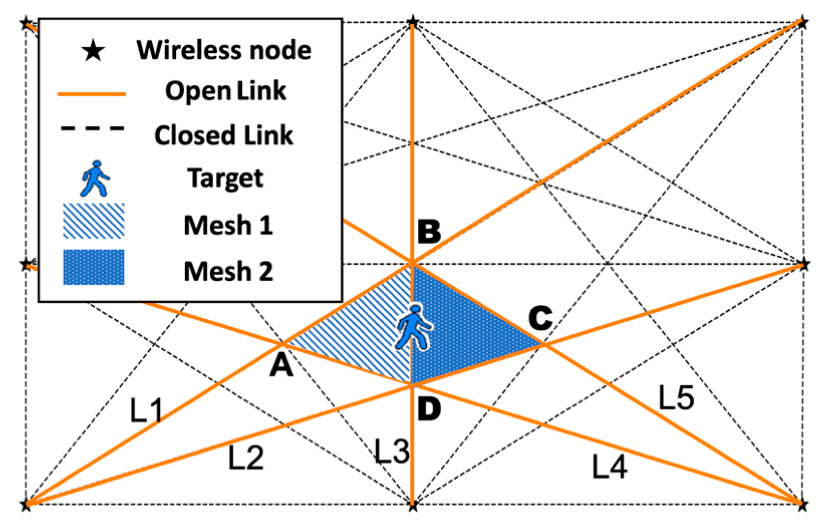
• The proposed scheme utilizes the mesh cluster to narrow the scope of monitoring by scanning only the mesh cluster-related wireless links and inactive remaining links, and the estimation of the target’s position is calculated by the weighted centroid coordinates of triggered meshes in the mesh cluster, which reduces energy consumption while ensuring positioning accuracy and noise interference.
• The performance of the proposed scheme is evaluated with groups of simulations under different parameters. Results demonstrate the accuracy and effectiveness of the method.

The remaining sections of this paper are organized as follows: Section 2 reviews the related works on RSS-based DFL. Section 3 introduces the system description and main structure of the IMC scheme. In Section 4, the performance of the proposed scheme is evaluated through simulations. Section 5 presents the computational complexity analysis. Finally, Section 6 provides conclusions and discusses future works.

2. Related Works

Several RSS-based DFL algorithms have been proposed in recent years, motivated by the diverse range of promising applications that can benefit from DFL. Fingerprint-based methods, as presented in [10,11,12,13], involve constructing a radio map through extensive offline training. During this training phase, RSS measurements are collected while a person stands at different locations. In the online phase, the current RSS measurements are compared with the radio map entries to infer the target’s location. However, these methods require significant manual calibration efforts during the offline phase. Statistical and probability methods, as presented in [14,15,16,17,18,19], employ a target-induced fading model that relies on the target’s proximity to the link. These models, derived through experimental data, are used in conjunction with particle filters to track the target’s location. The use of particle filters overcomes the restrictive assumptions made by Kalman filters regarding state space dynamics but introduces increased computational complexity. Radio tomographic imaging (RTI) methods, discussed in [20,21,22], approach DFL as an ill-posed image reconstruction problem that can be solved through regularization techniques. However, one drawback of these methods is that they often require significant computational resources, making them computationally intensive and potentially limiting their real-time applicability. The Bayesian grid approach (BGA) was introduced in [23] to address the DFL problem. While BGA offers advantages in utilizing lightweight operations on shadowing effect maps and incorporating prior and constraint information to obtain a location estimate, the drawback is that BGA may require a large amount of training data to accurately capture the prior and constraint information, which can be challenging and time-consuming to acquire in certain scenarios. To achieve high performance localization in sparsely deployed scenarios, compressive sensing (CS) theory [24,25,26] has been successfully utilized to model localization as a sparse signal reconstruction problem and accurately estimate the target’s location by solving the inversion problem. Although the CS-based indoor localization system could achieve good performance, one drawback is the high computational complexity involved. The process of signal reconstruction in CS-based indoor localization systems can be computationally demanding, potentially limiting their real-time implementation, or requiring significant computational resources.

Geometric methods, proposed in [27,28,29,30,31,32], employ a sensor-grid deployment and assess the overlap of shapes formed by shadowed links to estimate the target’s location. A drawback of these methods is the lack of prior information to filter subsequent location estimates, rendering them sensitive to noise. In [29], a Kalman filter is used in conjunction with location estimates derived from geometric methods to enhance tracking accuracy. Our previous work in [32] introduced a geometric midpoint algorithm that aims to solve the DFL problem in low-density wireless sensor networks. More recent years, machine learning and deep learning method based DFL methods are also proposed. In [33], the authors presented a method for accurate DFL in WSNs using convolutional deep belief network (CDBN) to extract important features from raw signals. The results showed a high accuracy of 98% even with reduced data dimensions and low signal-to-noise ratios (SNRs). Refs. [34,35,36,37] proposed deep learning-based methods for accurate DFL. The drawback of these approaches is that they often require a substantial amount of labeled training data, which can be time-consuming and costly to acquire. This reliance on large training datasets may limit their applicability in scenarios where collecting such data is challenging or impractical. Additionally, the computational complexity involved in training deep learning models for DFL can be significant, requiring powerful hardware resources for efficient training and deployment.

Unlike the previously mentioned geometric model based DFL algorithms, the proposed IMC method in this paper uses geometric objects such as line segments, points, mesh, and mesh clusters to build a bridge between the possible target’s location and the active subset of wireless links. This approach eliminates the need for continuous scanning of all wireless links, making it more robust to noise and reducing the number of computations and storage required.

3. Proposed IMC Algorithm

3.1. System Description

We consider a WSN comprising several wireless nodes as depicted in Figure 1. As the target moves across the RoI, it causes variations in the RSS values on subset of all wireless links, resulting in the shadowing of certain links. The shadowed links change as the target relocates to different positions. Hence, the DFL system can estimate the target’s position by utilizing the information derived from the variations in RSS measurements.

Under the framework of the proposed IMC algorithm, the presence of a single device-free target results in the shadowing of only a subset of wireless links. Specifically, the target is located within the segment BD, which corresponds to the boundary shared by Mesh1 and Mesh2. Subsequently, the target moves from this area to a different position along one of the four segments: AB, BC, CD, or DA. Consequently, only specific links require scanning, namely L1, L2, L3, L4, and L5, which correspond to the segments AB, BC, CD, AD, and BD, respectively. Thus, the scanning strategy is significantly optimized. While assuming scanning all 24 wireless links would typically take t time, the proposed approach reduces this time to only 5/24t, theoretically. Moreover, the energy consumption is also proportionally reduced to approximately 5/24 of the original value. The underlying idea is to establish relationships among meshes, segments, links, nodes, and intersecting points formed by links. Using these relationships, it becomes possible to infer the adjacent links surrounding the target and derive a reasonable estimation of its location.

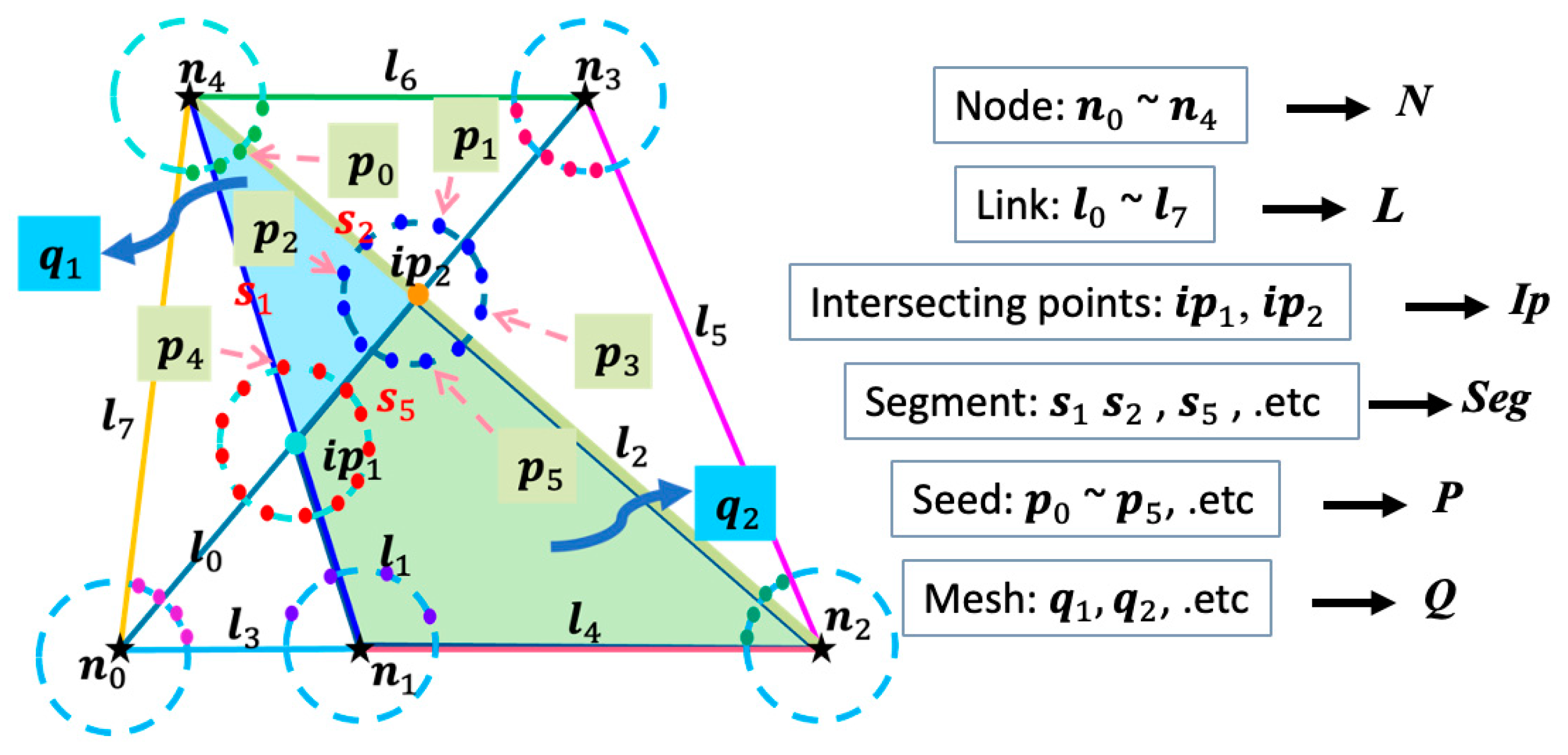
3.2. Geometric Elements Abstract

From a geometric perspective of WSNs, several key entities serve as the focal points of research in IMC model. These entities include wireless nodes, links, intersecting points, segments, meshes, and seed points that are the points generated around intersecting points and nodes. To facilitate a systematic and structured approach, we adopt the object-oriented programming method to abstract these research entities into classes. Specifically, the six main research objects are represented by the classes Node, Link, Ip (Intersecting Point), Segment, Seed, and Mesh. This abstraction enables a clear and organized representation of the underlying elements and their relationships within the IMC model.

(1) Node and Link: Building of Node class is the first step of intelligence mesh model. The attributes of Node class include id and coordinates of nodes. The created Node instances are stored in list N. Then build the Link class, the instance of Link connects pairwise nodes in the network. The built Link instances are temporarily stored in list L.

(2) Ip and Segment: The Ip (Intersecting Point) class represents the abstract of an intersecting point formed by the intersection of different links in a WSN. Using the list L, which contains link objects created in the previous step, the intersecting points are calculated using the Intersection-Point algorithm described in [32].

All intersecting points on a Link object are sorted in ascending order based on their x-axis coordinates. These points are then stored in the Ip list as an attribute of the corresponding Link instance, as illustrated in Figure 2a,b. Subsequently, instances of the Segment class are instantiated by connecting the sequenced intersecting points from the Ip list, including the two endpoints of the link.

For instance, considering the link depicted in red color in Figure 2b with endpoints ${\mathit{n}}_0$ and ${\mathit{n}}_1$, the first segment is formed by connecting node ${\mathit{n}}_0$ and intersecting point $\mathit{i}{\mathit{p}}_0$. The second segment connects intersecting point $\mathit{i}{\mathit{p}}_0$ with intersecting point $\mathit{i}{\mathit{p}}_1$, and the third segment starts at $\mathit{i}{\mathit{p}}_1$ and ends at $\mathit{i}{\mathit{p}}_2$. Finally, the last segment starts at $\mathit{i}{\mathit{p}}_2$ and ends at ${\mathit{n}}_1$. Similar segment lists are created for other links using the same approach. Furthermore, each newly created segment object is added to the Seg list as an attribute of the corresponding Link instance.

In addition to adding Segment instances as attributes to the Link instance, it is necessary to include these Segment instances in the list as attributes of the corresponding intersecting points. Figure 2b demonstrates this concept, where four segments are connected to intersecting point $\mathit{i}{\mathit{p}}_0$. Consequently, all four Segment instances should be added to the Seg list of intersecting point ip₀. Notably, segment ${\mathit{s}}_3$ is added not only to intersecting point $\mathit{i}{\mathit{p}}_0$ but also to $\mathit{i}{\mathit{p}}_1$.

Furthermore, during the creation of segment objects, the parent link attribute is assigned as a reference to the link that the current segment belongs to. This attribute is crucial as it aids in identifying the link based on its segments. For links situated at the boundary of the RoI, the segment list only contains the link itself as a sole member. The detailed process of generating the intersecting point list Ip and segments list Seg for each link in L is outlined in Algorithm 1.

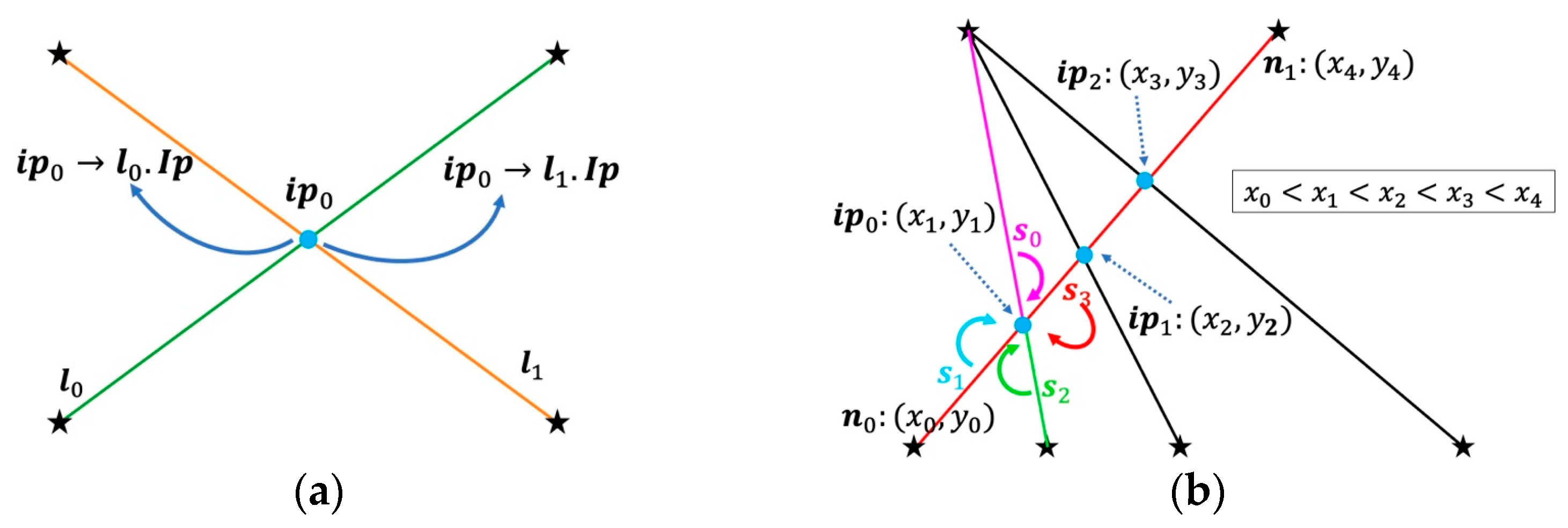
Algorithm 1 The method of creating Ip and Segment instances

Input: The list L including all Link instances in network.

Output: Intersecting point list Ip and Segments list Seg for each link in $\mathit{L}$.      1.  for all links ${\mathit{l}}_j$ in L do      2.        for all links ${\mathit{l}}_k$ in L, $j\ne k$ do      3.              Compute intersecting point $\mathit{c}\mathit{p}$ using Intersection-Point algorithm.      4.             if $\mathit{c}\mathit{p}\notin \left\{{\mathit{n}}_j^a,{\mathit{n}}_j^b,{\mathit{n}}_k^a,{\mathit{n}}_k^b\right\}$ then      5.                    ${\mathit{l}}_j.\mathit{I}\mathit{p}{{\displaystyle \cup }}^{}\left\{\mathit{c}\mathit{p}\right\}$      6.                    ${\mathit{l}}_k.\mathit{I}\mathit{p}{{\displaystyle \cup }}^{}\left\{\mathit{c}\mathit{p}\right\}$      7.  for all links ${\mathit{l}}_j$ in L do      8.                   Sort the intersecting points in $\mathit{I}\mathit{p}$ including two endpoints in ascending order of x-axis coordinates.      9.                    Create Segment instances with sequenced intersecting points and endpoints ${\mathit{n}}_j^a$ and ${\mathit{n}}_j^b$, then stored in Seg list.

(3) Seed and Mesh: The Seed class represents the generated points around intersecting points (Ips) and Node. The Mesh class abstracts the meshes formed by intersections among links in wireless network. Based on the intersecting point list Ip derived from all of the links and nodes in N, a set of Seed instances are generated at intersecting points and nodes on a circle with a radius of $r$, as depicted in Figure 3.

The creation of seed objects around the nodes involves a partial distribution on a circle. For nodes located at the four corners of the RoI, seeds should be generated within a range of approximately 90°. Similarly, for nodes positioned in the middle of the sides, the angle is approximately 180°, as shown in Figure 3a. The radius of the circle around all the nodes can be set to an appropriate value. Generally, a denser network with a larger number of nodes results in a smaller radius value. The main principle is to avoid overlapping between the current circle and the one surrounding intersecting points. On the other hand, the seeds created around intersecting points are uniformly distributed on the circle, as illustrated in Figure 3b. Each intersecting point is connected by four segments to neighboring intersecting points or nodes, as depicted in Figure 3c. The blue-colored intersecting point, labeled as $\mathit{i}{\mathit{p}}_1$, is connected to four segments (${\mathit{s}}_1$ to ${\mathit{s}}_4$) marked in blue. Similarly, the orange-colored intersecting point, labeled as ip₂, is connected to four segments (${\mathit{s}}_1$ to ${\mathit{s}}_4$) marked in orange. Notably, segment ${\mathit{s}}_4$ in blue and ${\mathit{s}}_3$ in orange are the same segment, as they connect both $\mathit{i}{\mathit{p}}_1$ and $\mathit{i}{\mathit{p}}_2$. To ensure there is no overlap between adjacent circles, the radius of the circle should meet the specified limitations, as defined:

$$r<\frac{1}{2}\min \left\{\left|\left|{\mathit{s}}_i\right|\right|\right\}, i=1,\dots ,4$$

(1)

where ${\mathit{s}}_1$ represents the four segments connected to the current intersecting point. $\left||·|\right|$ is Euclidean norm that is used to calculate the length of segment.

Once all the seeds have been created and stored in the list P as attributes for intersecting points or nodes, the next step involves calculating the positional relationship between each seed and all the links in the network. The general equation of a link is given by $Ax+By+C=0$, where the parameters $A$, B and $C$ are associated with the two endpoints of the link. Given a seed ${\mathit{p}}_i$ from the P list, with coordinates ($x_{{\mathit{p}}_i}$, $y_{{\mathit{p}}_i}$), the position relationship with link ${\mathit{l}}_j$ from the list L can be calculated as follows:

$${\varphi }_{ij}=\{\begin{array}{c}1, if(A_j{x}_{\mathit{p}i}+B_j{y}_{\mathit{p}i}+C_j>0) \\ 0, if(A_j{x}_{\mathit{p}i}+B_j{y}_{\mathit{p}i}+C_j=0)\\ -1, if(A_j{x}_{\mathit{p}i}+B_j{y}_{\mathit{p}i}+C_j<0)\end{array}$$

(2)

To illustrate this, we select a subset of seeds as depicted in Figure 4. In the given sketch map, there are eight links, and we choose six seeds distributed at different positions. By calculating the position relationship using Equation (2), the results are presented in

Table 1. The position relationship between seeds and links.

	Link	${\mathit{l}}_0$	${\mathit{l}}_1$	${\mathit{l}}_2$	${\mathit{l}}_3$	${\mathit{l}}_4$	${\mathit{l}}_5$	${\mathit{l}}_6$	${\mathit{l}}_7$
Seed
${\mathit{p}}_0$		1	1	−1	1	1	−1	−1	−1
${\mathit{p}}_1$		1	1	1	1	1	−1	−1	−1
${\mathit{p}}_2$		1	1	−1	1	1	−1	−1	−1
${\mathit{p}}_3$		−1	1	1	1	1	−1	−1	−1
${\mathit{p}}_4$		1	1	−1	1	1	−1	−1	−1
${\mathit{p}}_5$		−1	1	−1	1	1	−1	−1	−1

.

From the obtained results, it is observed that seeds ${\mathit{p}}_0$, ${\mathit{p}}_2$ and ${\mathit{p}}_4$ exhibit the same position relationship with all eight links. Therefore, these three seeds can be categorized into a single class. When creating seeds around the circle with the center at intersecting points or nodes, each generated seed possesses the attribute of the circle center. Consequently, given any generated seed, we can infer the corresponding intersecting point or node.

Based on this mechanism, by iteratively finding the center point for seeds ${\mathit{p}}_0$, ${\mathit{p}}_2$ and ${\mathit{p}}_4$ in the class, we can deduce the circle centers center ${\mathit{n}}_4$, $\mathit{i}{\mathit{p}}_2$, and $\mathit{i}{\mathit{p}}_1$, respectively. Subsequently, an instance of the Mesh class can be created with vertices at ${\mathit{n}}_4$, $\mathit{i}{\mathit{p}}_2$, and $\mathit{i}{\mathit{p}}_1$. Additionally, since the intersecting points $\mathit{i}{\mathit{p}}_2$ and $\mathit{i}{\mathit{p}}_1$, as well as the node ${\mathit{n}}_4$, possess attributes about the connected segments, by iteratively identifying the duplicate segment, we can readily determine that the sides of the newly created mesh are composed of segments ${\mathit{s}}_1$, ${\mathit{s}}_2$, and ${\mathit{s}}_5$.

Using the aforementioned approach, it becomes possible to create all the meshes within the network. The precise procedure for generating the seeds P and constructing the meshes Q is summarized in Algorithm 2.

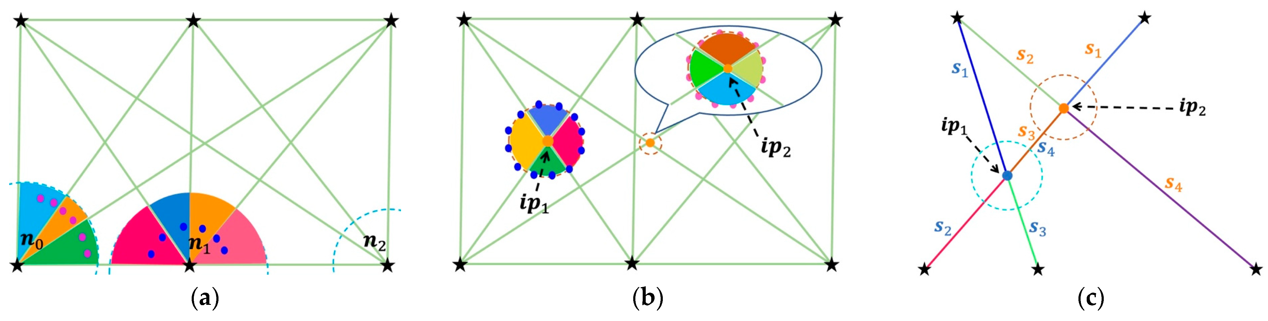
Algorithm 2 The method of creating Seed and Mesh instances

Input: All nodes N, intersecting points Ip, and links L.

Output: Seeds list P and meshes list Q.      1.  for all nodes ${\mathit{n}}_i$ in N do      2.        Create seeds ${\mathit{P}}^n$ around nodes ${\mathit{n}}_i$.      3.  for all intersecting points $\mathit{i}{\mathit{p}}_i$ in Ip do      4.  Create seeds ${\mathit{P}}^{ip}$ around intersecting points $\mathit{i}{\mathit{p}}_i$.      5.        $\mathit{P}={\mathit{P}}^n{{\displaystyle \cup }}^{}{\mathit{P}}^{ip}$      6.  for all seeds ${\mathit{p}}_i$ in $\mathit{P}$ do      7.           Calculate the position relationship ${\varphi }_{ij}$ with all links in L using Equation (2).      8.  Classify the seeds based on ${\varphi }_{ij}$, infer the vertexes and sides, then create meshes Q.

It is noted that when create new mesh instance, the reference of new mesh is also added to the meshes’ slide, that is segments or links on the edge of network. Also, it is possible to infer the corresponding link from a segment. Therefore, a mapping relation from a mesh ${\mathit{q}}_i$ to the links where its sides belong to is realized as

$$f\left({\mathit{q}}_i\right)=\left\{{\mathit{l}}_j\left|j=1,\dots ,\right|{\mathit{L}}_{{\mathit{q}}_i}\right|\}$$

(3)

where $\left|{\mathit{L}}_{{\mathit{q}}_i}\right|$ represents the quantity of mesh ${\mathit{q}}_i$ related links.

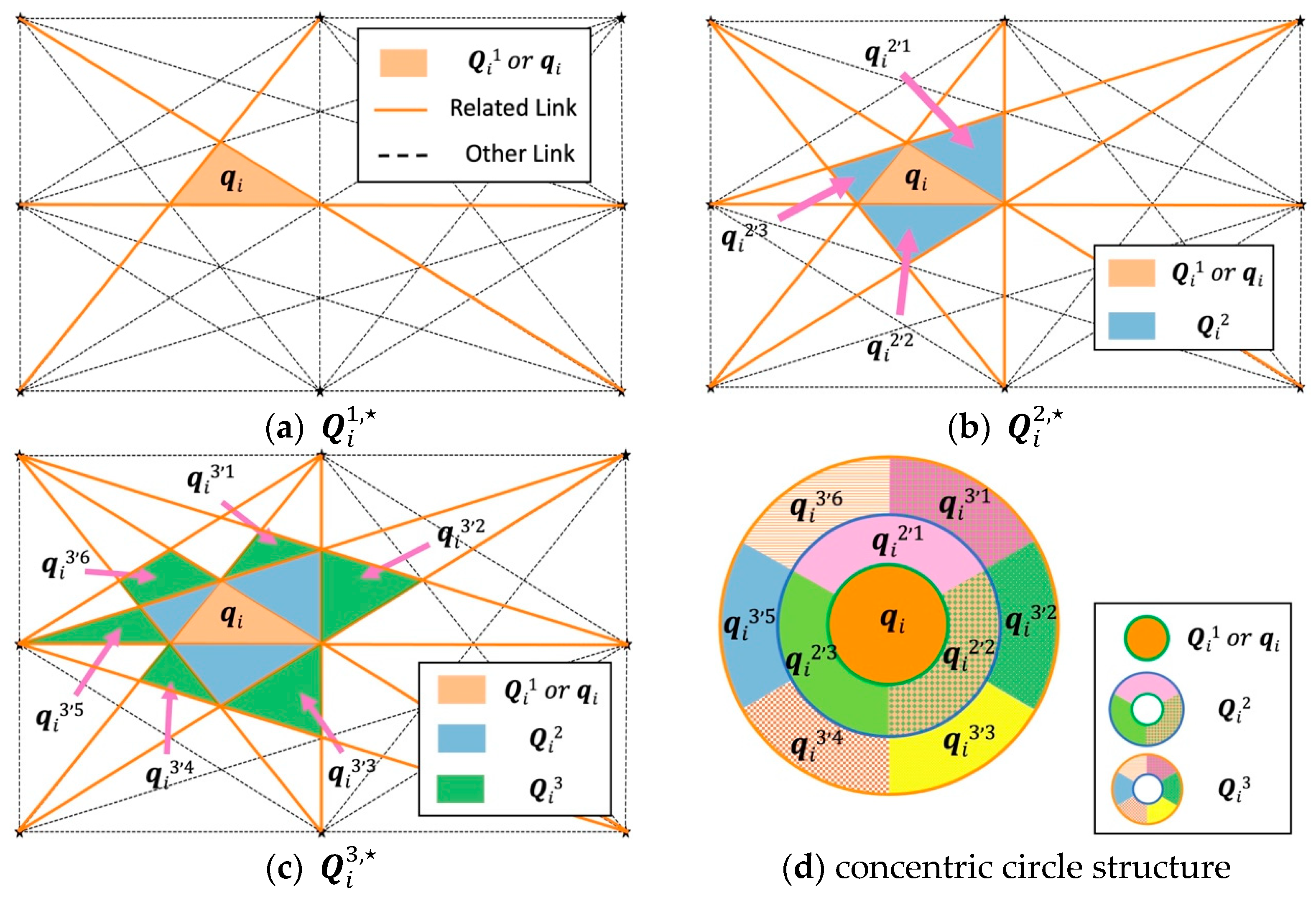
3.3. Mesh Cluster (MC) and Mesh Expansion Index (MEI)

When a target enters the region of interest covered by a WSN, typically the edge links are the first to be triggered. In order to achieve adaptive control of the links and activate only the related links in the area where the target is present while keeping other links inactive, the tracking process for the target should commence from the initially triggered edge links. Subsequently, the tracking can expand to include the connected meshes and their related links. As a result, we establish two definitions in this context:

Definition 1. 

The mesh cluster (MC)  ${\mathit{Q}}_{\mathit{i}}^{\eta , \star }$—a set of meshes that consists of a central mesh ${\mathit{q}}_i$ and the expanded neighbor meshes.

Definition 2. 

The mesh expansion index (MEI) $\eta$—the order (layer) of the neighbor meshes expanded from the central mesh ${\mathit{q}}_i$

.

For example, mesh cluster ${\mathit{Q}}_{\mathit{i}}^{\eta , \star }$ includes: central mesh ${\mathit{q}}_i$, and expanded meshes ${\mathit{Q}}_{\mathit{i}}^2$ on layer 2 to ${\mathit{Q}}_{\mathit{i}}^{\eta }$ on layer $\eta$. It should be noted that central mesh ${\mathit{q}}_i$ can also be represented as the mesh ${\mathit{Q}}_{\mathit{i}}^1$ on layer 1. ${\mathit{Q}}_{\mathit{i}}^{\eta }$ denotes a set of meshes that have the same MEI $\eta$ to central mesh ${\mathit{q}}_i$. The relation can be expressed in equation as:

$${\mathit{Q}}_i^{\eta ,\star }={\bigcup }_{k=1}^{\eta }{\mathit{Q}}_i^k={\mathit{Q}}_i^{\eta }{\displaystyle \cup }{\mathit{Q}}_i^{\eta -1}{\displaystyle \cup }\dots {\displaystyle \cup }{\mathit{Q}}_i^1$$

(4)

$${\mathit{Q}}_i^{\eta }=\left\{q_i^{\eta ,k}\right|k=1,\dots ,J_k\}$$

(5)

especially,

$${\mathit{Q}}_i^{1,\star }={\mathit{Q}}_i^1={\mathit{q}}_i$$

(6)

where symbol $\star$ represents the whole mesh members in all layers. $J_k$ represents the total number of the meshes in current layer. Intuitive examples for mesh cluster ${\mathit{Q}}_i^{1,\star }$, ${\mathit{Q}}_i^{2,\star }$, and ${\mathit{Q}}_i^{3,\star }$ are shown shown in Figure 5a–c. The structure of a mesh cluster can be abstracted as a concentric circle, and the innermost layer is the central mesh, and the other layers consist of the expanded neighbor meshes in different orders of mesh expansion index as shown in Figure 5d.

Given a mesh cluster ${\mathit{Q}}_i^{\eta ,\star }$, we can get the mesh cluster related links by

$${\mathit{L}}_{{\mathit{Q}}_i^{\eta ,\star }}={\bigcup }_{j=1}^{\left|{\mathit{Q}}_i^{\eta ,*}\right|}f\left({\mathit{q}}_j\right)$$

(7)

where function $f(·)$ is the mapping relation in Equation (3). $\left|{\mathit{Q}}_i^{\eta ,*}\right|$ represents the total number of meshes in mesh cluster ${\mathit{Q}}_i^{\eta ,*}$. It should be noted that there are no duplicate elements in ${\mathit{L}}_{{\mathit{Q}}_i^{\eta ,\star }}$. For example, the related links ${\mathit{L}}_{{\mathit{Q}}_i^{3,\star }}$ for mesh cluster ${\mathit{Q}}_i^{3,\star }$ are links in orange in Figure 5c.

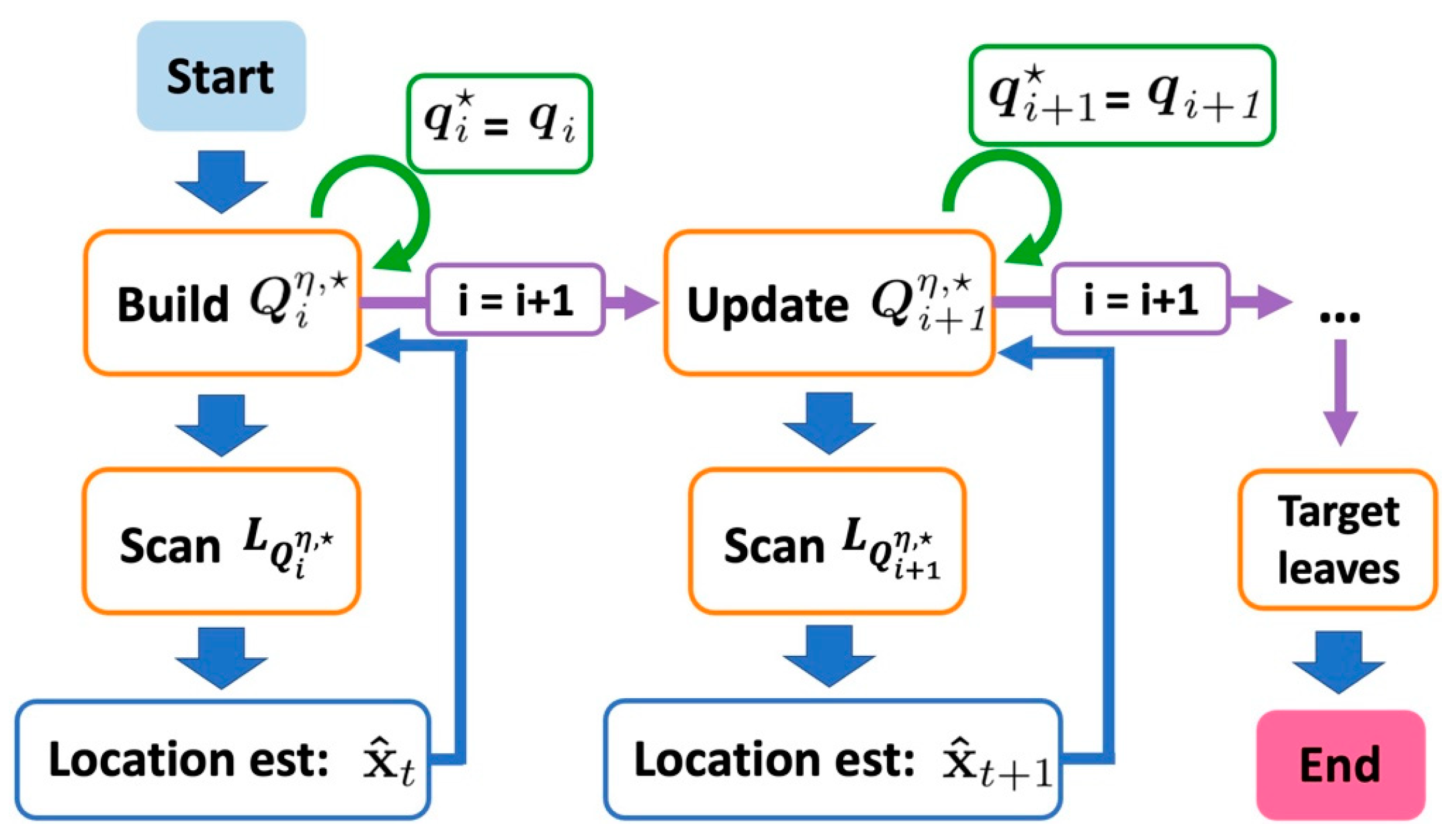
3.4. Location Estimation

The location estimation based on IMC algorithm is divided into two phases: the initialization of mesh cluster and the update of mesh cluster.

• Phase 1: Initialize mesh cluster.

Before the target enters the RoI, the system can only activate the edge links to save energy. Once one of the links is triggered, based on the triggered link’s neighbor mesh ${\mathit{q}}_i$, we build the first mesh cluster ${\mathit{Q}}_i^{\eta ,\star }$. Then the system turns to scan the mesh cluster related links ${\mathit{L}}_{{\mathit{Q}}_i^{\eta ,\star }}$. If there is any links in ${\mathit{L}}_{{\mathit{Q}}_i^{\eta ,\star }}$are triggered, the target location estimate $\widehat{x}$ will be calculated. The location estimate is calculated by weighted average of the centroid coordinate of triggered links related meshes in ${\mathit{Q}}_i^{\eta ,trig}$. The detailed algorithm about determining the ${\mathit{Q}}_i^{\eta ,trig}$ is introduced as follows.

Firstly, the central mesh ${\mathit{q}}_i$ is the first element in the set ${\mathit{Q}}_i^{\eta ,trig}$. The system scans the links in ${\mathit{L}}_{{\mathit{Q}}_i^{\eta ,\star }}$, and if any links are triggered by the target, the triggered links are saved in set ${\mathit{L}}_{{\mathit{Q}}_i^{\eta ,trig}}$. Then, we utilize ${\mathit{L}}_{{\mathit{Q}}_i^{\eta ,trig}}$ to find the related meshes ${\mathit{Q}}_i^{\eta ,trig}$, which is a subset of ${\mathit{Q}}_i^{\eta ,\star }$.

Starting with the central mesh ${\mathit{q}}_i$, we examine the segments set ${\mathit{q}}_i.$Seg around ${\mathit{q}}_i$. For each segment ${\mathit{s}}_j$ in ${\mathit{q}}_i.$Seg, we verify if the parent link ${\mathit{s}}_j.\mathit{l}$ for segment ${\mathit{s}}_j$ belong to the part of the triggered links ${\mathit{L}}_{{\mathit{Q}}_i^{\eta ,trig}}$. If the answer is yes, then, we add the newly discovered neighbor mesh to ${\mathit{Q}}_i^{\eta ,trig}$. Otherwise, we proceed to evaluate the next segment ${\mathit{q}}_i.$Seg. Similarly, we continue evaluating the next mesh in ${\mathit{Q}}_i^{\eta ,trig}$ until recursion stops.

The complete process of finding the triggered links’ related meshes is actually the process of building and traversal of an n-ary tree as shown in Figure 6. When building the n-ary tree, the root node of the n-ary tree is the central mesh ${\mathit{q}}_i$, and the other meshes in ${\mathit{Q}}_i^{\eta ,\star }$ are the leaf nodes at corresponding heights of the tree based on the parameter MEI $\eta$. The n-ary tree is traversed by depth-first search (DFS). In DFS, backtracking is used for traversal. In this traversal, the deepest node is visited first and then backtracks to its parent node if no siblings of that node exist. In the mesh cluster, DFS can be interpreted as searching from a segment of ${\mathit{q}}_i$ to a related neighbor mesh until no related neighbor meshes are found, and then backtracking to the next segment of ${\mathit{q}}_i$. It is also noted that the minimum set of ${\mathit{Q}}_i^{\eta ,trig}$ is $\left\{{\mathit{q}}_i\right\}$, when the set ${\mathit{L}}_{{\mathit{Q}}_i^{\eta ,trig}}$ is null.

The procedure of search tree algorithm is summarized in Algorithm 3.

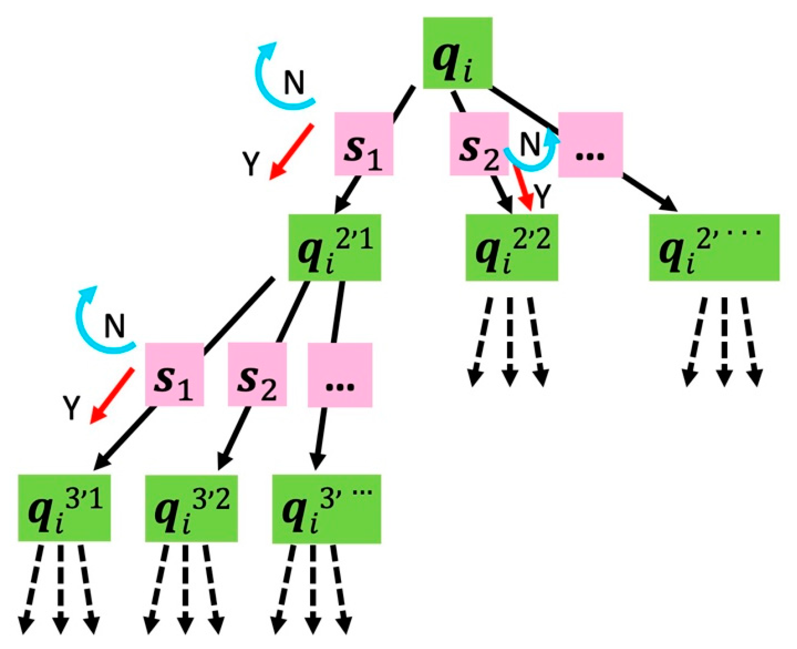
Algorithm 3 A n-Ary Tree Traversal Algorithm

Input: The mesh cluster ${\mathit{Q}}_i^{\eta ,*}$ and triggered links ${\mathit{L}}_{{\mathit{Q}}_i^{\eta ,trig}}$

Output: The set of triggered links related meshes ${\mathit{Q}}_i^{\eta ,trig}$      1.  Add the first item to ${\mathit{Q}}_i^{\eta ,trig} \leftarrow main mesh q_i$      2.  for all mesh ${\mathit{q}}_i$ in ${\mathit{Q}}_i^{\eta ,trig}$ do      3.          for all segment ${\mathit{s}}_j$ in ${\mathit{q}}_i.$Seg do      4.                if ${\mathit{s}}_j.\mathit{l}\in {\mathit{L}}_{{\mathit{Q}}_i^{\eta ,trig}}$ then      5.                      Add the neighbor mesh of segment ${\mathit{s}}_j$ into ${\mathit{Q}}_i^{\eta ,trig}$ without duplicate.

• Phase 2: Update mesh cluster.

We have determined the triggered links related meshes ${\mathit{Q}}_i^{\eta ,trig}$ in phase 1. Due to the environmental noise interference, we need to define a distance-based weight to improve the capacity of resisting disturbance. Simply speaking, the meshes in ${\mathit{Q}}_i^{\eta ,trig}$ except central mesh ${\mathit{q}}_i$ that have shorter centroid coordinate distance to ${\mathit{q}}_i$ should have larger weight value in calculating the location estimate. The distance-based weight is computed as

$$w_i^{k_1,k_2}=\frac{1}{\left|\left|x_{{\mathit{q}}_i^{k_1,k_2}}-x_{q_i}\right|\right|}$$

(8)

where $x_{{\mathit{q}}_i^{k_1,k_2}}$ and $x_{q_i}$ are the centroid coordinates of mesh ${\mathit{q}}_i^{k_1,k_2}$ and ${\mathit{q}}_i$, respectively. $\left||·|\right|$ is the Euclidean norm, and $k_1=2,\dots ,\eta , k_2=1,\dots ,\gamma$. $\eta$ is mesh expansion index. $\gamma$ is the number of meshes in corresponding level.

The location estimate at time t is calculated as

$${\widehat{x}}_t={{\displaystyle \sum }}_{i=1}^{\left|{\mathit{Q}}_i^{\eta ,trig}\right|}{w}_i\times x_{{\mathit{q}}_i^{k_1,k_2}}$$

(9)

where $w_i=\frac{w_i^{k_1,k_2}}{{\displaystyle \sum }{w}_i^{k_1,k_2}}$ are the normalized weights, $\left|{\mathit{Q}}_i^{\eta ,trig}\right|$ denotes the cardinality of the set ${\mathit{Q}}_i^{\eta ,trig}$, and $x_{{\mathit{q}}_i^{k_1,k_2}}$ represents the centroid coordinate of the mesh ${\mathit{q}}_i^{k_1,k_2}$.

After the location estimate ${\widehat{x}}_t$ is calculated by the mesh cluster ${\mathit{Q}}_i^{\eta ,\star }$, it needs to be used to update and determine the next mesh cluster ${\mathit{Q}}_{i+1}^{\eta ,\star }$. For all mesh members ${\mathit{q}}_i^{k_1,k_2}$ in mesh cluster ${\mathit{Q}}_i^{\eta ,\star }$, we calculate the distance from centroid coordinate to location estimate ${\widehat{x}}_t$ and find the corresponding mesh ${\mathit{q}}_i^{*}$ that has the minimum distance to ${\widehat{x}}_t$

$${\mathit{q}}_i^{*}=\underset{{\mathit{q}}_i^{k_1,k_2}}{\mathit{arg}\min }d\left(x_{{\mathit{q}}_i^{k_1,k_2}}, {\widehat{x}}_t\right)$$

(10)

where $d(·)$ represents the Euclidean distance operation.

If the ${\mathit{q}}_i^{*}$ and the central mesh ${\mathit{q}}_i$ is the same mesh, the system will keep scanning the links in ${\mathit{L}}_{{\mathit{Q}}_i^{\eta ,\star }}$ and calculate new location estimate rather than update mesh cluster ${\mathit{Q}}_{i+1}^{\eta ,\star }$. On the contrary, if the ${\mathit{q}}_i^{*}$ and the central mesh ${\mathit{q}}_i$ are not the same, the ${\mathit{q}}_i^{*}$ will be selected as the central mesh ${\mathit{q}}_{i+1}$ for updating the new mesh cluster ${\mathit{Q}}_{i+1}^{\eta ,\star }$. The process of building ${\mathit{Q}}_{i+1}^{\eta ,\star }$ with the mesh expansion index $\eta$ is the same with building ${\mathit{Q}}_i^{\eta ,\star }$. As soon as the mesh cluster ${\mathit{Q}}_{i+1}^{\eta ,\star }$ is built, the system turns to scan the links ${\mathit{L}}_{{\mathit{Q}}_{i+1}^{\eta ,\star }}$, which is calculated by Equation (7) based on the mesh cluster ${\mathit{Q}}_{i+1}^{\eta ,\star }$. In this way, the system can calculate the location estimate continuously in real time as the target moves until it leaves the RoI. The complete work flowchart is shown in Figure 7.

The procedure of the proposed IMC algorithm is summarized in Algorithm 4.

Algorithm 4 Intelligent Mesh Cluster Algorithm

1.  Network initialization: Build Nodes N, and Links L.      2.  Build Ips Ip and Segments Seg for each link using Algorithm 1.      3.  Build Seeds P for each intersecting points and nodes, Meshes Q using Algorithm 2.      4.  Scan the edge links of the network and build the first mesh cluster ${\mathit{Q}}_{\mathit{i}}^{\eta ,\star }$.      5.  Scan the links in ${\mathit{L}}_{{\mathit{Q}}_i^{\eta ,\star }}$ and calculate the location estimate ${\widehat{x}}_t$ using Equation (9).      6.  Find the nearest mesh ${\mathit{q}}_i^{*}$ using Equation (10).      7.  if ${\mathit{q}}_i^{*}$ is ${\mathit{q}}_i$ then      8.            Go back to step (7).      9.  else      10.            Update the next mesh cluster ${\mathit{Q}}_{i+1}^{\eta ,\star }$ and go back to step (7).

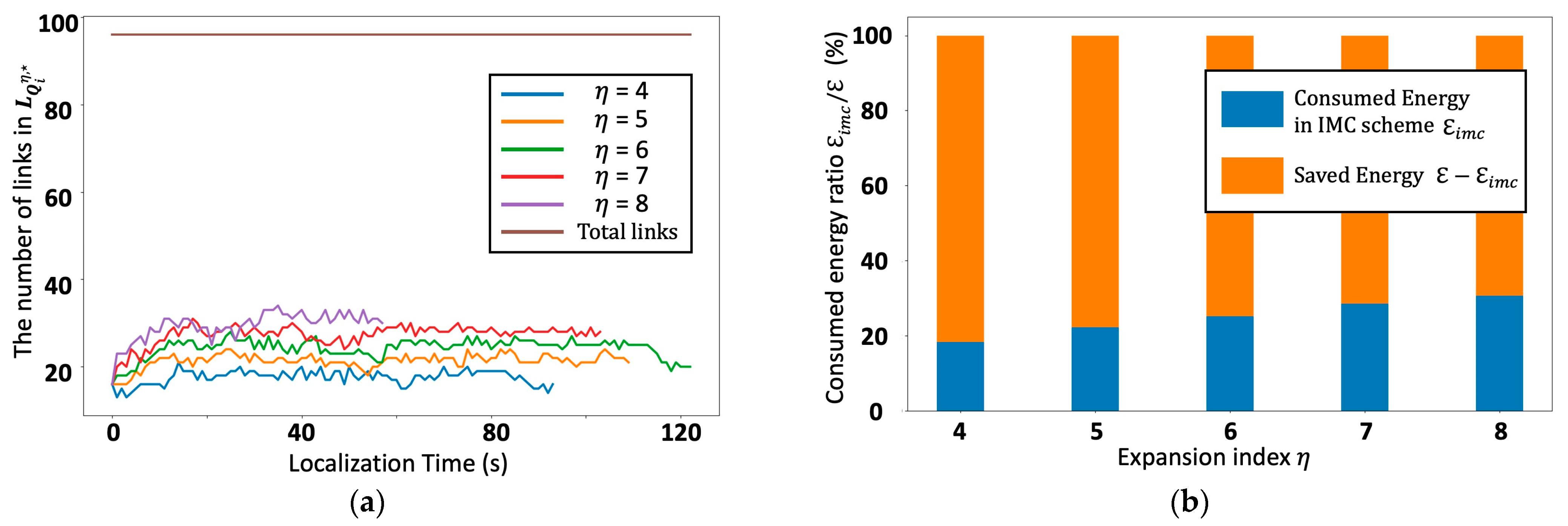
4. Performance Analysis and Evaluation

In this section, we evaluate the performance of the proposed IMC algorithm based DFL system with simulation analysis. We compare the proposed scheme with a conventional signal dynamic model based DFL system in terms of energy consumption and location estimation accuracy. To evaluate the performance of the IMC scheme, we designed four typical courses and simulated them under different system parameters. Some of the simulation results are shown in Figure 8.

The average error of the estimated target location is defined as

$$\mathsf{\epsilon }=\frac{1}{K_s}{{\displaystyle \sum }}_{k=1}^{K_s}\sqrt{{\left(x_k-{\widehat{x}}_k\right)}^2+{\left(y_k-{\widehat{y}}_k\right)}^2}$$

(11)

where $K_s$ is the total number of samples, $x_k$ and $y_k$ are the actual target location coordinates of the x-axis and y-axis, ${\widehat{x}}_k$ and ${\widehat{y}}_k$ are the estimated x and y coordinates at sample time $k$.

In order to test the anti-interference performance of the proposed algorithm, we designed a group of simulations. As shown in Section 3.4, the system only scans a subset of links in ${\mathit{L}}_{{\mathit{Q}}_i^{\eta ,\star }}$. We give a concept to describe noise interference level which is defined as

Definition 3. 

The interference level ($IL$) equals the number of links in ${\mathit{L}}_{{\mathit{Q}}_i^{\eta ,\star }}$ that have the inverse state compared to the actual triggered state.

In the ideal situation, there is no environmental interference and all links in ${\mathit{L}}_{{\mathit{Q}}_i^{\eta ,\star }}$ are triggered by the target, at this time, $IL=0$. The noise interference become more serious as the value $IL$ increases.

In our previous work [38], we discussed the power consumption model for the wireless communication links among the wireless nodes in the WSN. For a single wireless link with length $d$, the received power $P_r$ in Watt at receiver node is represented in the terms of antenna as:

$$P_r\left(d\right)=\frac{P_t{G}_t{G}_r{\lambda }^2}{{\left(4\pi \right)}^2{d}^2\gamma }$$

(12)

where $P_t$ is the transmitted power in Watt, $G_t$ and $G_r$ are the antenna gains for the transmitter and receiver, $\lambda$ is radio carrier wavelength, $\gamma$ is a constant system loss factor. The model can also be represented in units of dBm as:

$$P_R\left(d\right)=P_T-20\lg d+\varphi +X_n$$

(13)

where $P_T$ and $P_R$ are the transmitted and received power in dBm, respectively. $\varphi ={\log }_{10}\frac{G_t{G}_r{\lambda }^2}{{\left(4\pi \right)}^2\gamma }$ is a constant value related to the system, $X_n$ is a random variable that obeys a zero-mean Gaussian distribution. Due to variations in the lengths of wireless links within the WSN and the complexity of calculating energy loss consumed by the system itself, we focus solely on the energy consumption attributed to mesh cluster-related wireless links during the localization process. Assume the energy consumption for scanning all the wireless links in $\mathit{L}$ in turn is $\epsilon$, the energy consumption ${\epsilon }_{imc}$ with the scanning strategy under the proposed IMC scheme can be represented as follows:

$${\epsilon }_{imc}= \frac{\left|{\mathit{L}}_{{\mathit{Q}}_i^{\eta ,\star }}\right|}{\left|L\right|}·\epsilon$$

(14)

where ${\mathit{L}}_{{\mathit{Q}}_i^{\eta ,\star }}$ is described in Equation (7); $\mathsf{\epsilon }\approx \frac{N\left(N-1\right)}{2}·P_r·t$, in which N equals the quantity of wireless nodes in the WSN, $t$ is localization process time.

The average number of opened links $\left|{\mathit{L}}_{{\mathit{Q}}_i^{\eta ,\star }}\right|$ during the localization process is shown in Figure 9a. The energy ratio ${\epsilon }_{imc}/\epsilon$ about the saved energy in IMC scheme with conventional scan strategy is shown in Figure 9b. The proposed IMC scheme demonstrates significantly reduced energy consumption, approximately 20% to 30% compared to the conventional wireless link scanning strategy.

The performance of the proposed method under different parameter settings, namely Mesh Cluster Expansion Index $\eta$ and standard distance $\lambda$, in an ellipse model proposed in [20] is illustrated in Figure 10. Figure 10a demonstrates the impact of increasing Mesh Cluster Expansion Index $\eta$ on the system’s localization accuracy. As $\eta$ increases, the system exhibits improved accuracy in localizing the target. However, Figure 9a suggests that excessively large values of $\eta$ may lead to the loss of the target. Through simulation experience, it has been determined that the system achieves stable and accurate tracking performance when $\eta$ is set to 6 or 7. Figure 10b focuses on the effect of different values of standard distance $\lambda$ in the ellipse model on tracking accuracy. It is observed that both extremely large and extremely small values of $\lambda$ result in decreased tracking accuracy. The optimal value for λ in this scenario is approximately 2.5.

The mean tracking error and cumulative distribution function (CDF) [39] for the proposed algorithm are compared with RTI [20,21,22], BGA [23], GF [30], and sequential importance resampling (SIR) particle filter [16], as illustrated in Figure 11. The simulation results demonstrate the effectiveness of the proposed algorithm.

5. Computational Complexity Analysis

The IMC algorithm leverages geometric relationships among various objects, such as nodes, links, segments, intersecting points, seeds, meshes, and mesh clusters. These relationships are utilized to combine wireless link triggering, link switching, and mesh cluster conversion processes to achieve DFL target tracking. Importantly, this approach does not require a complex building model or the storage of a substantial amount of RSS data from all wireless links simultaneously.

In the view of algorithms, according to Algorithms 1 and 2, the running time is dominated by the two-layer loop to calculate the intersecting points and create the seed around these points, which is related to the quantity of the wireless links $L$, whose complexity is $O\left(L^2\right)$. The classification algorithm (line 8) in Algorithm 2 is used to classify the arrays including 0, 1, and −1 with the same array length to classify seeds, introducing a complexity of $O\left(L\right)$. In the localization process, the computational complexity for the n-Ary Tree traversal algorithm in Algorithm 3 is $O\left(K\right)$. A traversal of a tree touches every node in the tree once, by definition. If there are K tree nodes, the time complexity is $O\left(K\right)$. Overall, the total computational complexity is $O\left(L^2+L+K\right)$.

In the BGA and RTI schemes, an $M\times N_g$ matrix is computed offline to generate an image representing target-induced shadowing within the deployment area. BGA employs addition and multiplication operations on a series of vectors to estimate the target’s location. However, in BGA, the $N_g\times 1$ prior region must be constructed at each iteration, even for grids where the target is highly unlikely to be located.

6. Conclusions and Future Work

In this study, we proposed an IMC algorithm aimed to solve the DFL problem. Inspired by the object-oriented programming idea of Python, we divide the WSN into different intelligent modules, which can exchange more information and improve the ability to detect target of the monitored system. The algorithm can localize the targets based on the predetermined transforming relationship of all meshes and realize energy saving by only scanning parts of targets related links, which is also achieved through the relationship of meshes and links. The simulation results show that the proposed IMC algorithm has achieved accurate positioning and decrease the energy consumption than conventional DFL scheme.

In the future, the practical implementation of the IMC algorithm is a crucial aspect that requires in-depth exploration. As for the proposed scheme is to be used in practice, it is important for achieving accurate switching between different mesh cluster-related wireless link groups, while also maintaining continuous tracking of device-free targets as they move within the region of interest. Real-world deployment and extensive field testing will be necessary to validate its performance under various environmental conditions and network scenarios.

References

1. Yang, J.; Wang, M.; Yang, Y.; Wang, J. A device-free localization and size prediction system for road vehicle surveillance via UWB networks. IEEE Trans. Instrum. Meas. 2022, 71, 1–11. [Google Scholar] [CrossRef]
2. Feng, Y.S.; Liu, H.Y.; Hsieh, M.H.; Fung, H.C.; Chang, C.Y.; Yu, C.C.; Huang, C.W. An RSSI-based device-free localization system for smart wards. In Proceedings of the 2021 IEEE International Conference on Consumer Electronics-Taiwan (ICCE-TW), Penghu, Taiwan, 15–17 September 2021; pp. 1–2. [Google Scholar]
3. Ma, L.; Liu, M.; Wang, H.; Yang, Y.; Wang, N.; Zhang, Y. WallSense: Device-free indoor Localization using wall-mounted UHF RFID tags. Sensors 2019, 19, 68. [Google Scholar] [CrossRef] [Green Version]
4. Cimdins, M.; Schmidt, S.O.; Hellbrück, H. MAMPI-UWB—Multipath-assisted device-free localization with magnitude and phase information with UWB transceivers. Sensors 2020, 20, 7090. [Google Scholar] [CrossRef]
5. Lee, J.; Park, K.; Kim, Y. Deep learning-based device-free localization scheme for simultaneous estimation of indoor location and posture using FMCW radars. Sensors 2022, 22, 4447. [Google Scholar] [CrossRef]
6. Park, K.; Lee, J.; Kim, Y. Deep learning-based indoor two-dimensional localization scheme using a frequency-modulated continuous wave radar. Electronics 2021, 10, 2166. [Google Scholar] [CrossRef]
7. Yang, S.; Kim, Y. Single 24-GHz FMCW radar-based indoor device-free human localization and posture sensing with CNN. IEEE Sens. J. 2023, 23, 3059–3068. [Google Scholar] [CrossRef]
8. Yang, S.; Sun, C.; Kim, Y. Indoor 3D localization scheme based on BLE signal fingerprinting and 1D convolutional neural network. Electronics 2021, 10, 1758. [Google Scholar] [CrossRef]
9. Konings, D.; Faulkner, N.; Alam, F.; Lai, E.M.-K.; Demidenko, S. FieldLight: Device-free indoor human localization using passive visible light positioning and artificial potential fields. IEEE Sens. J. 2020, 20, 1054–1066. [Google Scholar] [CrossRef]
10. Youssef, M.; Mah, M.; Agrawala, A. Challenges: Device-free passive localization for wireless environments. In Proceedings of the 13th Annual ACM International Conference on Mobile Computing and Networking (MobiCom’07), Montreal, QC, Canada, 9–14 September 2007; pp. 222–229. [Google Scholar]
11. Moussa, M.; Youssef, M. Smart devices for smart environments: Device-free passive detection in real environments. In Proceedings of the 2009 IEEE International Conference on Pervasive Computing and Communications, Galveston, TX, USA, 9–13 March 2009; pp. 1–6. [Google Scholar]
12. Seifeldin, M.; Saeed, A.; Kosba, A.E.; El-Keyi, A.; Youssef, M. Nuzzer: A large-scale device-free passive localization system for wireless environments. IEEE Trans. Mob. Comput. 2013, 12, 1321–1334. [Google Scholar] [CrossRef] [Green Version]
13. Zhang, D.; Liu, Y.; Guo, X.; Ni, L.M. RASS: A real-time, accurate, and scalable system for tracking transceiver-free objects. IEEE Trans. Parallel Distrib. Syst. 2013, 24, 996–1008. [Google Scholar] [CrossRef]
14. Wilson, J.; Patwari, N. A fade-level skew-laplace signal strength model for device-free localization with wireless networks. IEEE Trans. Mob. Comput. 2012, 11, 947–958. [Google Scholar] [CrossRef] [Green Version]
15. Nannuru, S.; Li, Y.; Zeng, Y.; Coates, M.; Yang, B. Radio-frequency tomography for passive indoor multitarget tracking. IEEE Trans. Mob Comput. 2013, 12, 2322–2333. [Google Scholar] [CrossRef]
16. Wang, J.; Gao, Q.; Yu, Y.; Cheng, P.; Wu, L.; Wang, H. Robust device-free wireless localization based on differential RSS measurements. IEEE Trans. Ind. Electron. 2013, 60, 5943–5952. [Google Scholar] [CrossRef]
17. Guo, Y.; Huang, K.; Jiang, N.; Guo, X.; Li, Y.; Wang, G. An exponential-rayleigh model for RSS-based device-free localization and tracking. IEEE Trans. Mob. Comput. 2015, 14, 484–494. [Google Scholar] [CrossRef]
18. Li, Y.; Chen, X.; Coates, M.; Yang, B. Sequential monte carlo radio-frequency tomographic tracking. In Proceedings of the 2011 IEEE International Conference on Acoustics, Speech and Signal Processing (ICASSP), Prague, Czech Republic, 22–27 May 2011; pp. 3976–3979. [Google Scholar]
19. Kaltiokallio, O.J.; Hostettler, R.; Patwari, N. A novel bayesian filter for RSS-based device-free localization and tracking. IEEE Trans. Mob. Comput. 2021, 20, 780–795. [Google Scholar] [CrossRef]
20. Wilson, J.; Patwari, N. Radio tomographic imaging with wireless networks. IEEE Trans. Mob. Comput. 2010, 9, 621–632. [Google Scholar] [CrossRef] [Green Version]
21. Wilson, J.; Patwari, N. See-through walls: Motion tracking using variance-based radio tomography networks. IEEE Trans. Mob. Comput. 2011, 10, 612–621. [Google Scholar] [CrossRef]
22. Kaltiokallio, O.; Bocca, M.; Patwari, N. A fade level-based spatial model for radio tomographic imaging. IEEE Trans. Mob. Comput. 2014, 13, 1159–1172. [Google Scholar]
23. Wang, J.; Gao, Q.; Cheng, P.; Yu, Y.; Xin, K.; Wang, H. Lightweight robust device-free localization in wireless networks. IEEE Trans. Ind. Electron. 2014, 61, 5681–5689. [Google Scholar] [CrossRef]
24. Feng, C.; Au, W.S.A.; Valaee, S.; Tan, Z. Received-signal-strength-based indoor positioning using compressive sensing. IEEE Trans. Mob. Comput. 2012, 11, 1983–1993. [Google Scholar] [CrossRef]
25. Wang, J.; Gao, Q.; Wang, H.; Cheng, P.; Xin, K. Device-free localization with multidimensional wireless link information. IEEE Trans. Veh. Technol. 2015, 64, 356–366. [Google Scholar] [CrossRef]
26. Wang, J.; Chen, X.; Fang, D.; Wu, C.Q.; Yang, Z.; Xing, T. Transferring compressive-sensing-based device-free localization across target diversity. IEEE Trans. Ind. Electron. 2015, 62, 2397–2409. [Google Scholar] [CrossRef]
27. Zhang, D.; Ma, J.; Chen, Q.; Ni, L. An RF-based system for tracking transceiver-free objects. In Proceedings of the 5th Annual IEEE International Conference on Pervasive Computing and Communications (PerCom’07), White Plains, NY, USA, 19–23 March 2007; pp. 135–144. [Google Scholar]
28. Zhang, D.; Lu, K.; Mao, R.; Feng, Y.; Liu, Y.; Ming, Z.; Ni, L. Fine-grained localization for multiple transceiver-free objects by using RF-based technologies. IEEE Trans. Parallel Distrib. Syst. 2014, 25, 1464–1475. [Google Scholar] [CrossRef]
29. Talampas, M.; Low, K. Geometry-based algorithms for device-free localization with wireless sensor networks. In Proceedings of the 2014 IEEE Ninth International Conference on Intelligent Sensors, Sensor Networks and Information Processing (ISSNIP), Singapore, 21–24 April 2014; pp. 1–6. [Google Scholar]
30. Talampas, M.; Low, K. A geometric filter algorithm for robust device-free localization in wireless networks. IEEE Trans. Ind. Inform. 2016, 12, 1670–1678. [Google Scholar] [CrossRef]
31. Talampas, M.C.R.; Low, K.S. An enhanced geometric filter algorithm with channel diversity for device-free localization. IEEE Trans. Instrum. Meas. 2016, 65, 378–387. [Google Scholar] [CrossRef]
32. Sun, C.; Zhou, B.; Yang, S.; Kim, Y. Geometric midpoint algorithm for device-free localization in low-density wireless sensor networks. Electronics 2021, 10, 2924. [Google Scholar] [CrossRef]
33. Abdullah, O.A.; Al-Hraishawi, H.; Chatzinotas, S. Deep learning-based device-free localization in wireless sensor networks. In Proceedings of the 2023 IEEE Wireless Communications and Networking Conference (WCNC), Glasgow, UK, 26–29 March 2023. [Google Scholar]
34. Zhou, R.; Hou, H.; Gong, Z.; Chen, Z.; Tang, K.; Zhou, B. Adaptive device-free localization in dynamic environments through adaptive neural networks. IEEE Sens. J. 2021, 21, 548–559. [Google Scholar] [CrossRef]
35. Zhao, L.; Huang, H.; Li, X.; Ding, S.; Zhao, H.; Han, Z. An accurate and robust approach of device-free localization with convolutional autoencoder. IEEE Internet Things J. 2019, 6, 5825–5840. [Google Scholar] [CrossRef]
36. Abdull Sukor, A.S.; Kamarudin, L.M.; Zakaria, A.; Abdul Rahim, N.; Sudin, S.; Nishizaki, H. RSSI-based for device-free localization using deep learning technique. Smart Cities 2020, 3, 444–455. [Google Scholar] [CrossRef]
37. Koutris, A.; Siozos, T.; Kopsinis, Y.; Pikrakis, A.; Merk, T.; Mahlig, M.; Papaharalabos, S.; Karlsson, P. Deep learning-based indoor localization using multi-view BLE signal. Sensors 2022, 22, 2759. [Google Scholar] [CrossRef]
38. Zhou, B.; Ahn, D.; Lee, J.; Sun, C.; Ahmed, S.; Kim, Y. A passive tracking system based on geometric constraints in adaptive wireless sensor networks. Sensors 2018, 18, 3276. [Google Scholar] [CrossRef] [PubMed] [Green Version]
39. Stark, H.; Woods, J.W. Probability, Statistics, and Random Processes for Engineers, 4th ed.; Pearson Education: London, UK, 2011. [Google Scholar]
Figure 1. DFL system made up of eight nodes.
Electronics 12 03426 g001
Figure 2. Illustration for the process of building intersecting points list Ip as (a) and segments list Seg as (b).
Electronics 12 03426 g002
Figure 3. Illustration of the Seed creation process: (a) Partial distribution of Seeds around Nodes on a circle, (b) Uniform distribution of Seeds around intersecting points on a circle, (c) Intersecting points connected by Four Segments to neighboring intersecting points or nodes.
Electronics 12 03426 g003
Figure 4. Illustration for the relationship among segments, seeds, and meshes.
Electronics 12 03426 g004
Figure 5. Illustration for the structure of a mesh cluster and the corresponding open links when the mesh cluster has different MEI η based on the same central mesh central mesh q i . (a) mesh cluster Q i 1 , . (b) mesh cluster Q i 2 , . (c) mesh cluster Q i 3 , . (d) abstracted concentric circle structure of Q i 3 , .
Electronics 12 03426 g005
Figure 6. Illustration for the process of building and traversal of an n-ary tree.
Electronics 12 03426 g006
Figure 7. Illustration for the complete work flowchart of the location estimate.
Electronics 12 03426 g007
Figure 8. Illustration for simulation results for tracking the target in six different target trajectories. (a) Course1: Square wave-shaped trajectory. (b) Course2: Sinusoidal wave-shaped trajectory. (c) Course3: Square rotary trajectory. (d) Course4: Circle rotary trajectory.
Electronics 12 03426 g008
Figure 9. Parameter influence analysis graph. (a) The number of opened links under different mesh expansion index η as the target moves. (b) The comparison of energy consumption with different mesh expansion index η .
Electronics 12 03426 g009
Figure 10. Parameter influence analysis graph. (a) Cumulative distribution function (CDF) under different Mesh Cluster Expansion Index η . (b) Cumulative distribution function under different standard distance λ in ellipse model.
Electronics 12 03426 g010
Figure 11. Results graphs compared to other approaches. (a) Mean tracking error under different schemes. (b) CDF of tracking error under schemes.
Electronics 12 03426 g011