Article

Study on Parking Space Recognition Based on Improved Image Equalization and YOLOv5

1
School of Automobile and Traffic, Shenyang Ligong University, Shenyang 110159, China
2
School of Information Science and Engineering, Shenyang Ligong University, Shenyang 110159, China
*
Author to whom correspondence should be addressed.
Electronics 2023, 12(15), 3374; https://doi.org/10.3390/electronics12153374
Submission received: 1 July 2023 / Revised: 2 August 2023 / Accepted: 4 August 2023 / Published: 7 August 2023
(This article belongs to the Special Issue Computer Vision for Modern Vehicles)

Abstract

:
Parking space recognition is an important part in the process of automatic parking, and it is also a key issue in the research field of automatic parking technology. The parking space recognition process was studied based on vision and the YOLOv5 target detection algorithm. Firstly, the fisheye camera around the body was calibrated using the Zhang Zhengyou calibration method, and then the corrected images captured by the camera were top-view transformed; then, the projected transformed images were stitched and fused in a unified coordinate system, and an improved image equalization processing fusion algorithm was used in order to improve the uneven image brightness in the parking space recognition process; after that, the fused images were input to the YOLOv5 target detection model for training and validation, and the results were compared with those of two other algorithms. Finally, the contours of the parking space were extracted based on OpenCV. The simulations and experiments proved that the brightness and sharpness of the fused images meet the requirements after image equalization, and the effectiveness of the parking space recognition method was also verified.

1. Introduction

Parking recognition is an important component of automatic parking systems. With the continuous increase in car ownership, parking difficulties have become one of the serious problems faced by urban sustainable development [1]. Due to the continuous changes in the surrounding environment, especially in dark environments with insufficient lighting at night, there is a large area of blurred vision, and parking under such conditions becomes more difficult.
Deep learning has been widely used in the field of computer vision and image processing in recent years. Zhang et al. [2] first proposed a parking space recognition method based on a DCNN (deep convolutional neural network); the method first used YOLOv2 [3] as a detector to detect parking space marker points, then obtained parking space orientation information through a custom classification network, and finally inferred the complete parking space, which had a stronger recognition ability than the previous method but had defects such as not being able to distinguish the occupancy of parking spaces, along with the computation process being tedious and complicated. Jang et al. [4] proposed a parking space detection method based on semantic segmentation with deep learning, which used a semantic segmentation network to classify objects such as vehicles, free space, and parking space markers, but using this method for detection requires a lot of time and cannot meet various needs during the actual parking process, as well as being unable to obtain sufficiently accurate results. Liu Ze [5] proposed a parking space detection model that was built based on Faster-RCNN. Although this model meets the demand for parking space recognition in daily parking sessions in terms of accuracy, the real-time aspect of parking space recognition in the automatic parking process still needs to be improved, because of the long computation time of the Faster R-CNN algorithm itself. With the iterative updating of YOLO [6] series target detection networks, whether compared with the Faster R-CNN [7] or SSD [8], YOLO has been widely used in the industry for its excellent detection speed and accuracy compared to the Faster R-CNN two-stage target detection network and the SSD one-stage target detection algorithm.
This article proposes an improved fusion algorithm based on vision and YOLOv5 target detection to improve the image equalization process to solve the problem of uneven image brightness in the process of parking space recognition, as well as providing a reliable basis for vehicle parking, so as to improve safety and reduce the rate of cutting when parking.

2. Camera Calibration and Projection Transformation

2.1. Camera Calibration

The location of the fisheye camera deployed on the experimental vehicle in this paper is shown in Figure 1.
In the calibration process of the monocular vision system, the internal reference of the camera is a very critical parameter, which directly reflects the mapping relationship from the environment to the image. It is assumed that there is a point p in the image and p(u,v) is its coordinates in the pixel coordinate system, while p(x,y) is its coordinates in the image coordinate system. In addition, there is a three-dimensional point Pc(xc, yc, zc) in the camera coordinate system. By deriving the relationships among the image coordinate system, the pixel coordinate system, the camera coordinate system, and the camera imaging model, the camera internal reference matrix can be obtained as follows:
z c u v 1 = f x 0 u 0 0 f y v 0 0 0 1 x c y c z c = K x c y c z c
u = x d x + u 0 v = y d y + v 0
where u 0 and v 0 represent the coordinates of the projection position of the camera lens’s optical axis in the pixel coordinate system; K is the internal reference matrix of the camera; f x = f / d x , f y = f / d y , f denotes the focal length of the camera, while d x and d y denote the width and height of the unit pixel, respectively.
In addition, the camera’s aberration needs to be considered in the camera calibration process, and the aberration of the camera can be expressed by the following equation:
x c o r r e c t e d = x ( 1 + k 1 r 2 + k 2 r 4 ) + 2 p 1 x y + p 2 ( r 2 + 2 x 2 ) y c o r r e c t e d = y ( 1 + k 1 r 2 + k 2 r 4 ) + 2 p 2 x y + p 1 ( r 2 + 2 y 2 )
where k 1 and k 2 stand for the first-order and second-order coefficients of radial distortion, respectively, p 1 and p 2 represent the first-order and second-order coefficients of tangential distortion, respectively, and x c o r r e c t e d and y c o r r e c t e d are the corrected coordinates, where r 2 = x 2 + y 2 , respectively.
The Zhang Zhengyou calibration method [9] obtains the mapping matrix by using the relationship between the feature points on the calibration plate and their corresponding feature points on the image coordinate system. The specific camera calibration results are shown in Table 1 and Table 2 below.
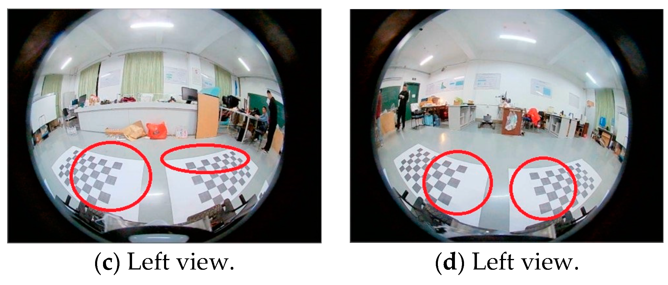
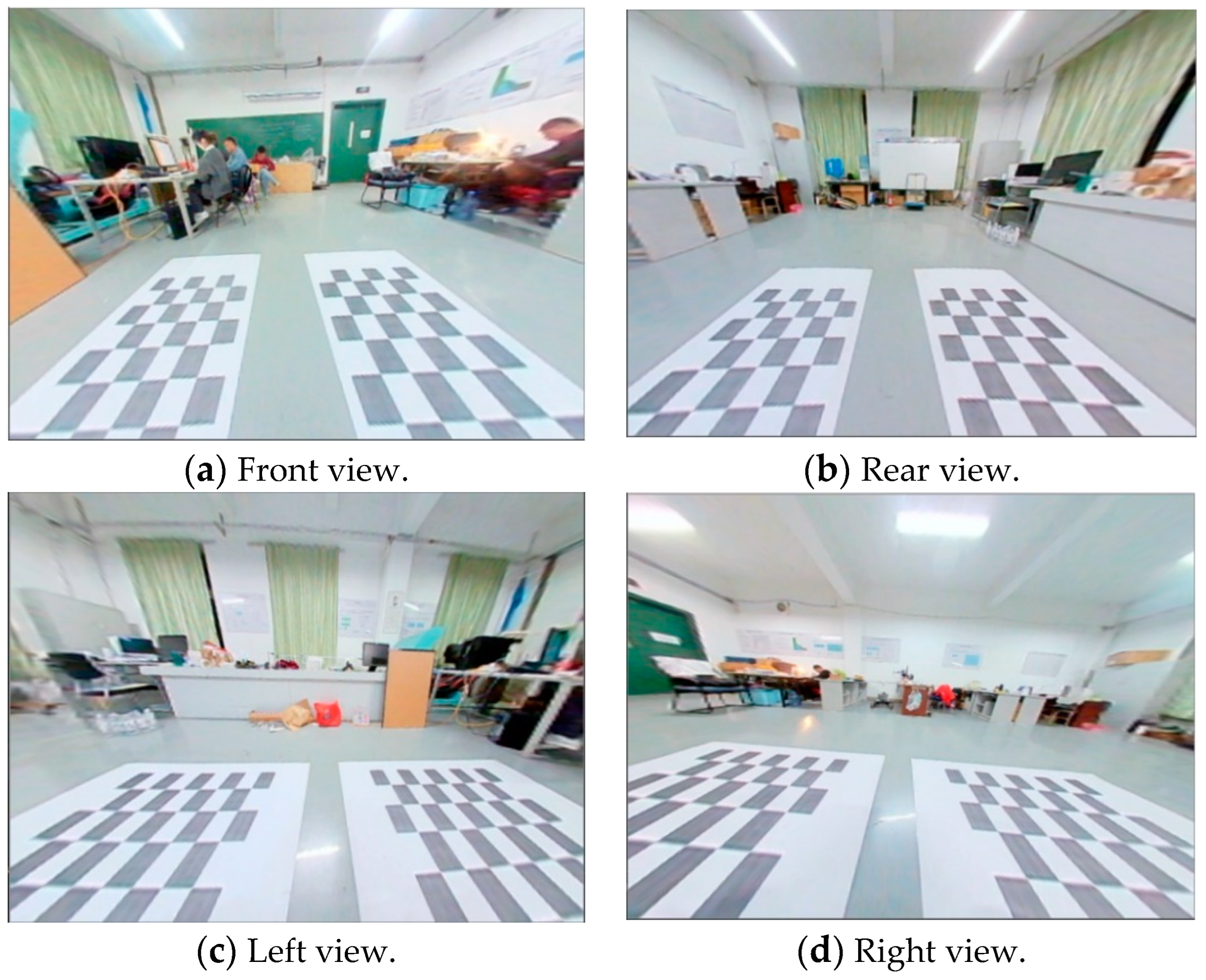
The aberration correction of the image is realized according to the camera’s internal reference and aberration coefficient obtained from the above table. Figure 2 below shows the original image, the red-circled area represents the part of the image with the larger distortion. Figure 3 shows the image after aberration correction.
As can be seen from the above two images, the distorted and aberrant images that existed in the red area of the original image were significantly corrected.

2.2. Projection Transformation

Direct linear transformation (DLT) [10] uses a homography matrix under image coordinate system and world coordinate system transformation to complete top-view transformation. The DLT single-shoulder mapping formula is shown below.
u = L 1 X + L 2 Y + L 3 Z + L 4 L 9 X + L 10 Y + L 11 Z + 1 v = L 5 X + L 6 Y + L 7 Z + L 8 L 9 X + L 10 Y + L 11 Z + 1
where L 1 , L 2 , L 11 are 11 unknown parameters of the single response matrix; u , v are the perspective image coordinates of the calibration point; X , Y , Z are the world coordinates of the calibration point, and when the world coordinate is the coordinate on the ground plane, it can be seen that Z = 0 , from which the top-down perspective transformation mapping formula can be obtained as shown in (5).
u = L 1 X + L 2 Y + L 4 L 9 X + L 10 Y + 1 v = L 5 X + L 6 Y + L 8 L 9 X + L 10 Y + 1
Rewriting the above equation into matrix form, the corresponding perspective image can be obtained by multiplying the points in world coordinates by the single response matrix. This can be expressed as Equation (6):
s u v 1 = L 1 L 2 L 4 L 5 L 6 L 8 L 9 L 10 1 X Y 1 = H X Y 1
where s is the scale factor and H indicates the single response matrix under this coordinate transformation. The image coordinates can be obtained by detecting the vertices of the four corners of the rectangle. To obtain the world coordinates, the size of the checkerboard grid and the distance of the checkerboard grid from the origin of the world coordinates are measured.
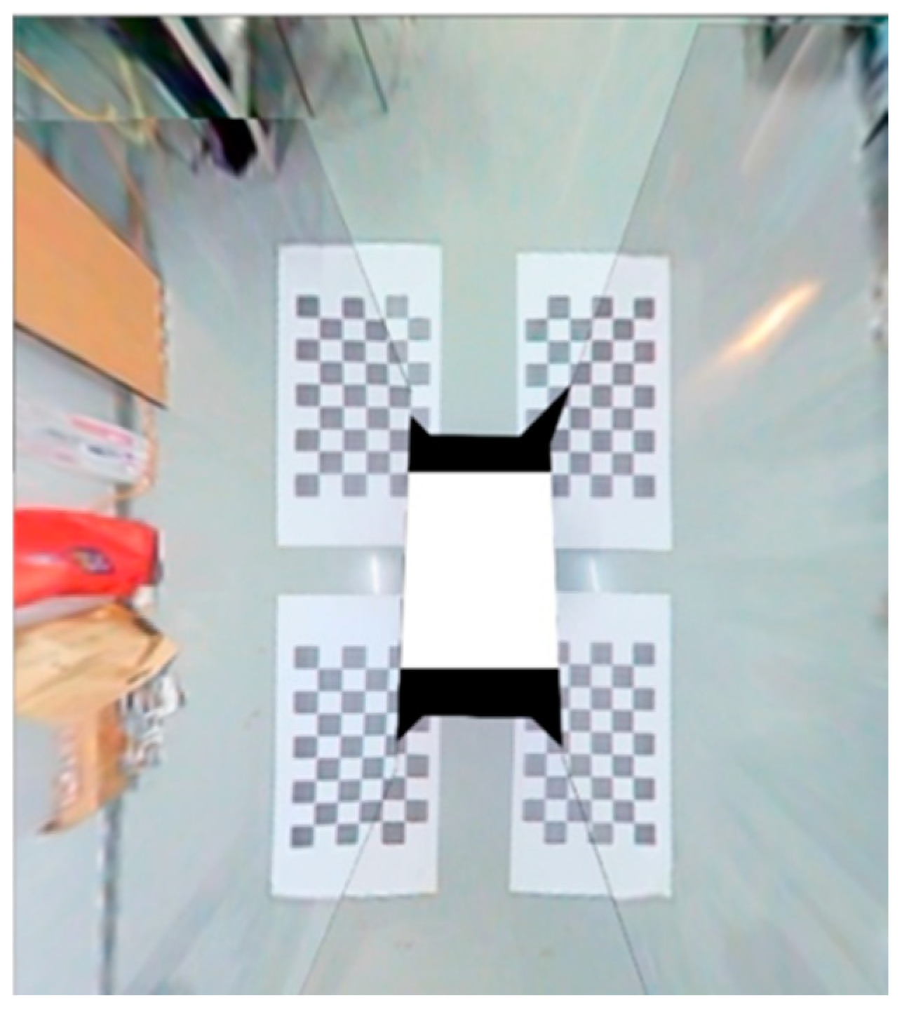
The projection matrices of the four cameras are not independent of one another, but to ensure that the projection points are positioned exactly in correspondence, we place the markers around the vehicle, acquire the images, manually select the corresponding points, and then obtain the projection matrix to achieve the next step of the top-view stitching. The projected transformed image is shown in Figure 4.

3. Image Stitching and Equalization Processing

3.1. Image Stitching

In image stitching, the image common point matching method cannot meet the demand for real-time operation due to its large computational volume [11]. In contrast, the stitching method based on a unified coordinate system can achieve fast real-time processing while ensuring accuracy. To stitch the four images together, a unified stitching coordinate system must be established first. The y-axis in Figure 5 indicates the ground projection corresponding to the line where the front and rear cameras are located, and the x-axis indicates the ground projection corresponding to the line where the left and right rear-view mirrors are located.
The four top views obtained from the projection transformation in the previous section are cropped and rotated according to their positions in the panorama, as shown in Figure 6.
After that, they are placed sequentially into the same coordinate system, as shown in Figure 7.
As can be seen in Figure 7, the panoramic-stitched top view has a large pixel difference at the stitching seam, which requires further fusion of the stitching.

3.2. Increase the Equalization Adjustment Factor

Next, the adjacent overlapping areas in the spliced image—that is, the four common areas of the front, rear, left, and right top views—are processed by the weighted average fusion method.
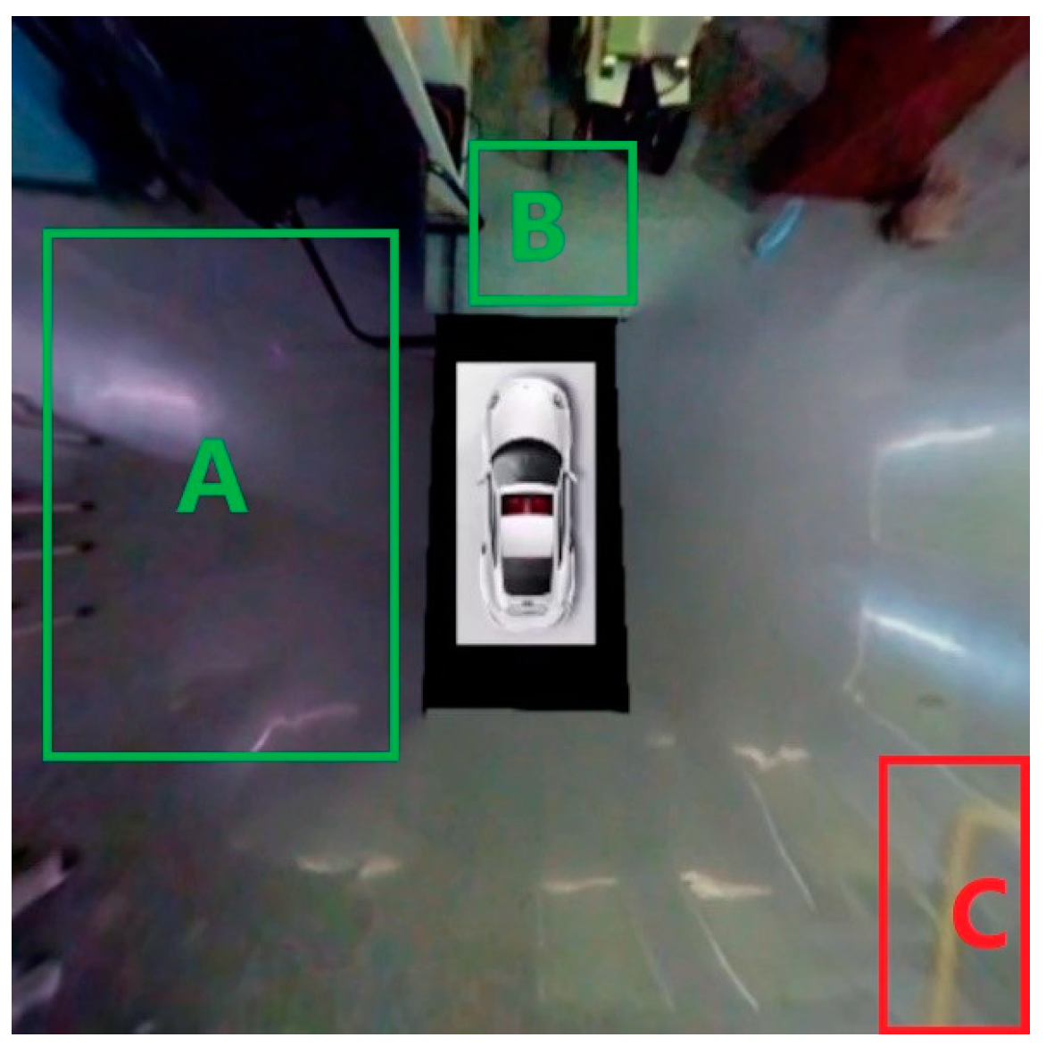
Figure 8 shows the fusion map obtained by weighted average fusion directly, without equalization processing, due to the exposure of different cameras and differences in light intensity in the surrounding environment; as a result, different regions will appear bright and dark, as shown in the green rectangular boxes in Figure 8A,B. A and B denote two brightness imbalance regions, and C denotes the car position blurring region.
The unadjusted equalization coefficients are derived from the luminance ratios of the four frames in the four overlapping regions.
x i = t i d i a i   ,   i = 1 , 2 , 3
y i = t i b i c i   ,   i = 1 , 2 , 3
z i = t i c i d i   ,   i = 1 , 2 , 3
w i = t i a i b i   ,   i = 1 , 2 , 3
t i = a i × b i × c i × d i 4 ,   i = 1 , 2 , 3
where a i denotes the average luminance ratio of the B, G, and R channels in the right-view area and the front-view area, and b i , c i , and d i are the average luminance ratios of the rear-view area and the right-view area, the average luminance ratios of the left-view area and the rear-view area, and the average luminance ratios of the front-view area and the left-view area, respectively; t i indicates the average luminance ratio of the B, G, and R channels of the image as a whole; x i indicates the equalization coefficients of the B, G, and R channels in the front-view area; similarly, there are also y i , z i , and w i equalization coefficients for the rear-view region, left-view region, and right-view region, respectively. Figure 9 shows the fusion map after the equalization process by the above equation. A1, B1, and C1 denote regions A, B, and C after general equalization.
The fusion map after the equalization process overall looks slightly more balanced in brightness, especially for the color difference changes in the A and B regions in Figure 8, and the A1 and B1 regions look more coherent in the whole image compared to the A and B regions. However, in terms of the yellow parking space line in the red rectangular box area (C1), it is still relatively fuzzy after the equalization process, and there is no obvious change in the clarity before and after the process, which, in turn, will adversely affect the subsequent parking space recognition.
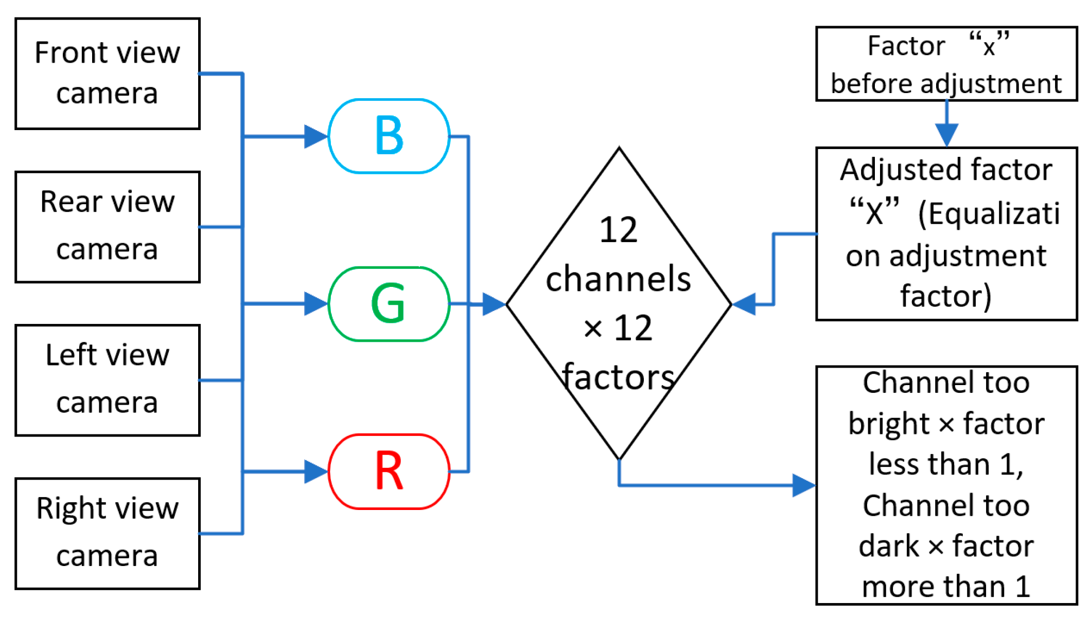
At this time, the brightness of each region needs to be adjusted so that the brightness of the whole stitched image tends to be stable. In this paper, we propose an improved image fusion method with the basic idea shown in Figure 10.
Each camera returns three channels of B, G, R, and the four cameras return a total of 12 channels. In order to perform equalization fusion, 12 adjustment coefficients are introduced; these coefficients are applied to the 12 channels, each channel is adjusted by multiplying them together, and finally the adjusted channels are combined to form the equalized fused picture. The adjustment coefficients are shown in the following equations:
X i = x i e 0.5 1 x i ,   x i 1 x i e 0.8 1 x i ,   x i < 1
Y i = y i e 0.5 1 y i ,   y i 1 y i e 0.8 1 y i ,   y i < 1
Z i = z i e 0.5 1 z i ,   z i 1 z i e 0.8 1 z i ,   z i < 1
W i = w i e 0.5 1 w i ,   w i 1 w i e 0.8 1 w i ,   w i < 1
where X i indicates the adjusted brightness coefficients of the B, G, and R channels in the front-view area, and Y i , Z i , and W i are the adjusted brightness coefficients of the rear-view area, left-view area, and right-view area, respectively. The coefficient x denotes the unadjusted equalization factor, i.e., x i ,   y i , z i , and w i in Equations (7)–(10), and the coefficient X denotes the adjusted equalization factor, i.e., X i , Y i , Z i , and W i in Equations (12)–(15), which is improved in this paper. The purpose of introducing the equalization adjustment coefficients is to darken the overly bright channels, so that the multiplication factor is less than 1, and the overly dark channels are brightened, so that the multiplication factor is greater than 1. Figure 11 shows the panoramic fusion of the improved image equalization process. C2 denotes the parking area obtained by the improved processing.
Compared with Figure 9, the yellow parking space line in the red area C2 in Figure 11 is obviously much clearer after the processing of the image equalization adjustment coefficient, and the brightness of the image is more balanced and stable. The experimental results show that this improvement improves both brightness and sharpness in image fusion compared with the results of the unadjusted equalization coefficient processing, and it can provide brightness-balanced picture inputs for the parking space recognition model.

4. YOLOv5-Based Parking Space Recognition Model

4.1. Experimental Environment Configuration

The YOLOv5 target detection algorithm [12,13] has been applied in different fields and scenarios, but there has been no specific application study for car space recognition at present. Considering the need for real-time detection of video streams, a model with a higher detection rate was selected to avoid lag during real-time detection, so YOLOv5s was finally chosen as the algorithm for automatic parking space recognition in this paper.
The hardware configuration information for this experiment is shown in Table 3.
The car parking recognition model training was based on the PyTorch framework, compiled using PyCharm, and the software environment configuration is shown in Table 4.

4.2. Model Training

Before conducting the training, the 1350 produced samples were randomly divided at a ratio of 7:3; 954 samples constituted the training set for training the model, and the remaining 396 samples constituted the validation set for verifying the effect of the model after training. The 1350 samples included a total of about 10,000 manually labeled instances in different scenarios, with two categories of empty and occupied parking spaces, labeled as vacant parking and occupied parking, respectively. The information statistics of the dataset are shown in Figure 12.
The top-left panel of Figure 12 shows the distribution of categories in the training set, and the overall distribution of instances in the two categories is relatively balanced, with sufficient and equal numbers of positive and negative samples.
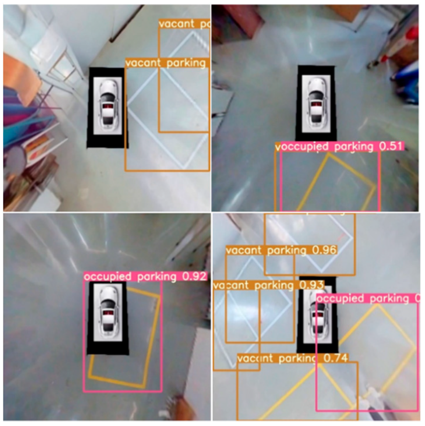
In this experiment, the official pre-training weights provided by YOLOv5s were used for training, the batch size was set to 16, the number of iterations was set to 100, and the resolution size of the input images was 640 × 640. Figure 13 shows the effects of some images in the YOLOv5s prediction test set, and the prediction box contains whether each parking space is occupied or not, along with its confidence level.
The brown box area in the above figure indicates an empty parking space, and the end of the label corresponds to the confidence level that it is an empty parking space, with a larger value closer to 1 indicating a higher probability of being an empty parking space. Similarly, the pink box area indicates an occupied parking space.

4.3. Analysis of Model Training Results

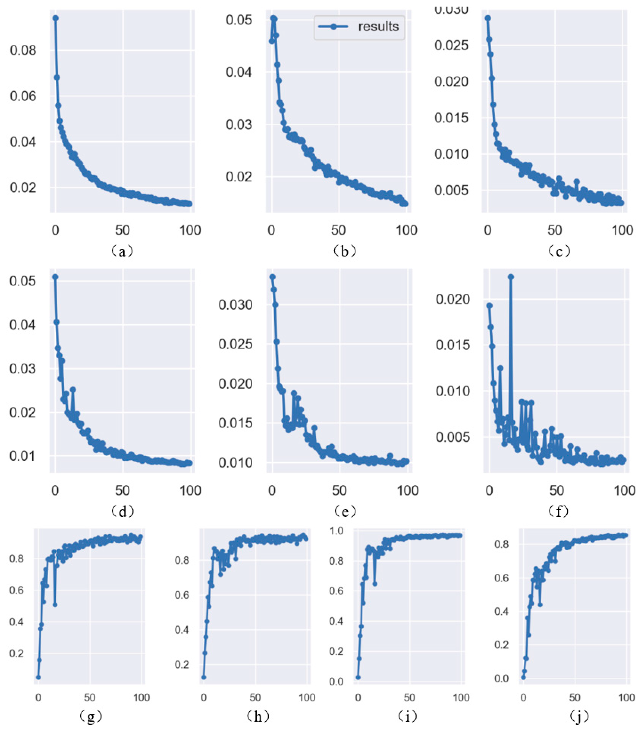
After 100 rounds of training, the evaluation results obtained by YOLOv5 were as shown in Figure 14.
The above plots show the evaluation results of the car space recognition model. In each vignette, the horizontal axis indicates the number of training rounds, the vertical axis indicates the corresponding parameter values, and mAP indicates the mean accuracy value. After 40 rounds of training, convergence of the model was observed, while after 100 rounds of training the parameters of the model stabilized and almost ceased to change. The accuracy and recall of the model steadily improved at the beginning of the iterations, and after 100 rounds each loss was oscillating downward, and the localization loss, target confidence loss, and category loss were all below 0.02. The recall of the model was maintained above 92%, the accuracy was fixed at about 94%, the mean accuracy reached 96%, and the training ended with vacant parking, occupied parking, and the overall mAP scores obtained after training. The datasets were also fed into the YOLOv7 [14] and YOLOv8 [15] algorithms for training and testing, respectively, and the results obtained were compared with those of YOLOv5, as shown in Table 5 below.
According to Table 5, it can be seen that the overall effect of YOLOv5 is the best. Although YOLOv8 has the best performance effect in mAP, it has average performance effects in accuracy and recall, and the difference between YOLOv5’s mAP and YOLOv8’s mAP is only 0.2%. YOLOv7, on the other hand, does not perform as well as YOLOv5 and YOLOv8 in any aspect of the evaluation metrics. YOLOv5 has an overall mAP of 96.6%, which reflects the overall good performance of this parking space recognition model. When performing parking space recognition, the average detection speed is 52.3 fps; 1 fps is equivalent to 0.304 m/s, so 52.3 fps is about 16 m/s, or 57 km/h, which is suitable for the task of real-time parking space recognition during automatic parking.

5. OpenCV-Based Car Parking Contour Line Extraction

5.1. Image Grayscale Processing

Image grayscale processing simplifies the image, highlights image details, and facilitates subsequent image processing and analysis tasks.
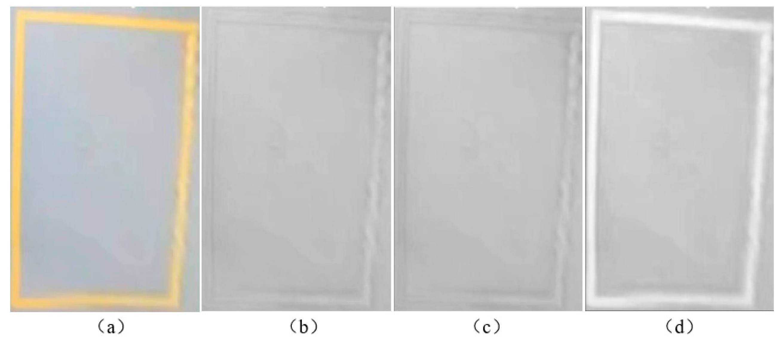
The weighted averaging method obtains the grayscale value of the point by weighting the luminance of the three channels R, G, and B of the image [16]. When using the maximum value method, the gray value of the point is taken as the value with the largest luminance among the three components of R, G, and B. When using the average value method, the gray value of the point is taken as the average value of the luminance of the three components of R, G, and B, as shown in Equations (16)–(18).
G r a y i , j = 0.299 R i , j + 0.587 G i , j + 0.114 B i , j
G r a y i , j = max R i , j , G i , j , B i , j
G r a y i , j = R i , j + G i , j + B i , j 3
where 0.299, 0.587, and 0.114 are the values of the regular coefficients of the human eye’s sensitivity to red, green, and blue colors, respectively. G r a y i , j represents the pixel value after gray scaling, and R i , j , G i , j , and B i , j represent the pixel values of the red, green, and blue channels of the original image, respectively. In this section, the car parking image is grayed out using the above three methods, and the results are shown in Figure 15.
The overall parking space image that is processed by using the maximum value method and the average value method is very fuzzy, so the parking space contour line and the surrounding pixels are not clearly distinguished from one another; compared with these two methods, the weighted average method can retain the parking space line contour of the original image well. The overall processing results are clearer and the details are retained more comprehensively, so we ultimately chose the weighted average method for the grayscale processing.

5.2. Image Filtering

Image filtering plays an important role in denoising, smoothing, and edge detection, helping to improve the quality, clarity, and visual impact of images.
Mean filtering, median filtering, and Gaussian filtering are three common filtering methods. In the mean filtering method, a 3 × 3 filter template is used to average the pixel values of the pixel point to be processed and the surrounding eight pixel points. On the other hand, the median filtering method is used to change the process of averaging pixel values in the mean filtering method to find the median value, which replaces the gray value of the pixel point to be processed with the median value. The Gaussian filtering method is used to eliminate Gaussian noise, using a filter template to scan each pixel point of the whole image. It determines the gray value of the pixel point to be processed by weighting the gray value of each pixel point within the template. In this section, the grayscale image is filtered using the above three methods, and the results are shown in Figure 16.
As shown in Figure 16, there is no obvious difference in the processing effect; all of them retain the basic outline of the original parking line and can effectively suppress the noise and retain the image details. But combined with the results of subsequent image binarization processing, the median filter has a better denoising effect on the image, which can provide clearer and more accurate image data for subsequent image binarization processing and analysis. Therefore, the median filter was ultimately selected for the filtering process.

5.3. Image Binarization Processing

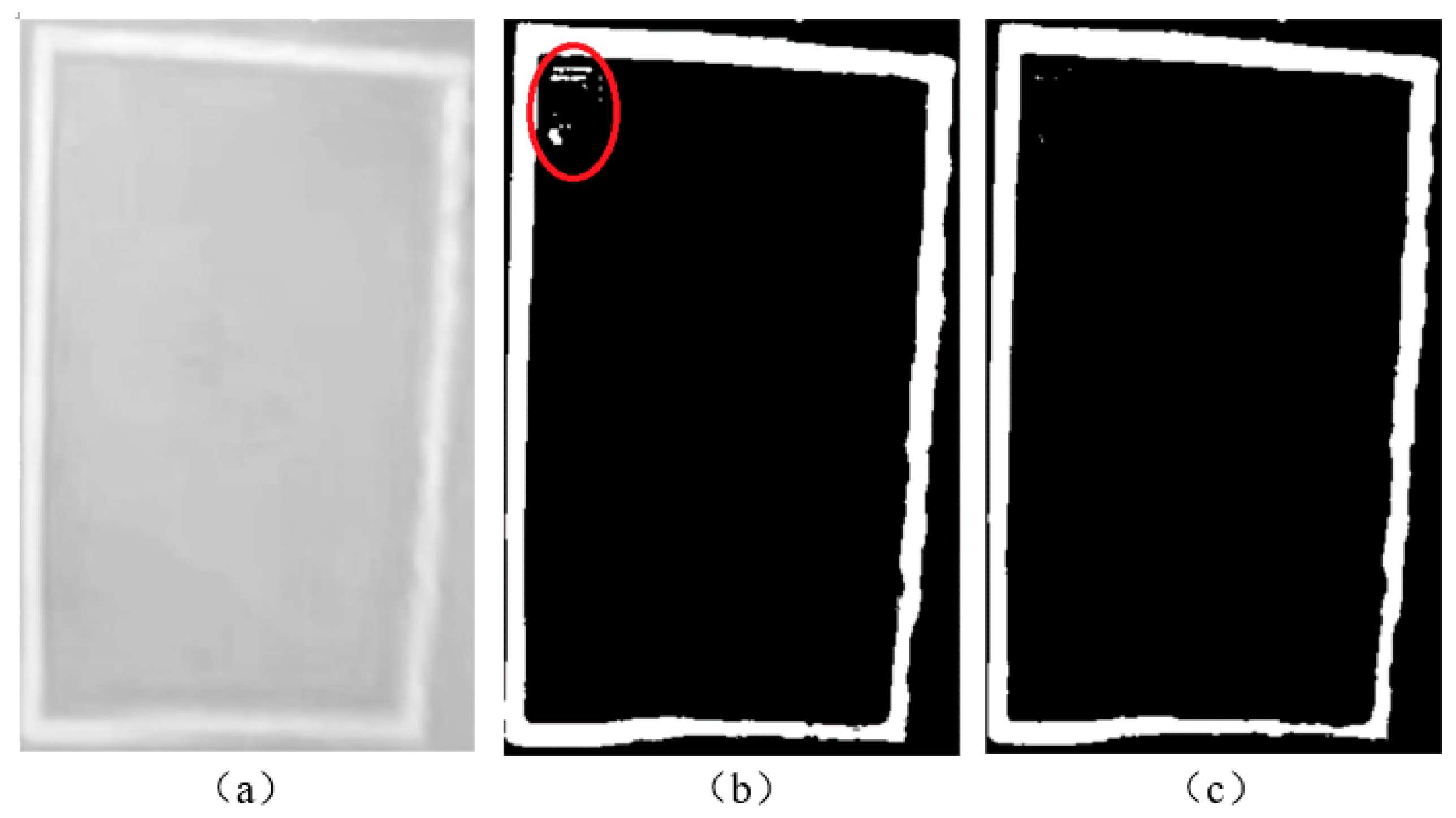
Since a large number of parking images need to be processed, the brightness and the color of the parking images change from scene to scene, and the fixed threshold method is not applicable in this case.
Two global adaptive methods for calculating thresholds are provided in the OpenCV library: (1) cv2.THRESH_OTSU, which uses the maximum interclass variance method to find an appropriate threshold for the image, and (2) cv2.THRESH_TRIANGLE, which uses histogram data to find the optimal threshold based on purely geometric methods. In this section, the filtered image is binarized using the above two methods, and the result is shown in Figure 17. The red circle indicates areas with large noise.
The parking space contour lines are basically extracted after the processing of the two adaptive binarization methods, but as far as the red box area in (b) is concerned, the parking space image after TRIANGLE adaptive binarization has obvious noise, which will have an impact on the next morphological processing operation. On the other hand, the parking space image after OTSU adaptive binarization processing basically retains the parking space line contour information completely and removes the individual larger noise successfully, and most of the background information is effectively segmented, so OTSU was ultimately selected for binarization processing.

5.4. Morphological Processing

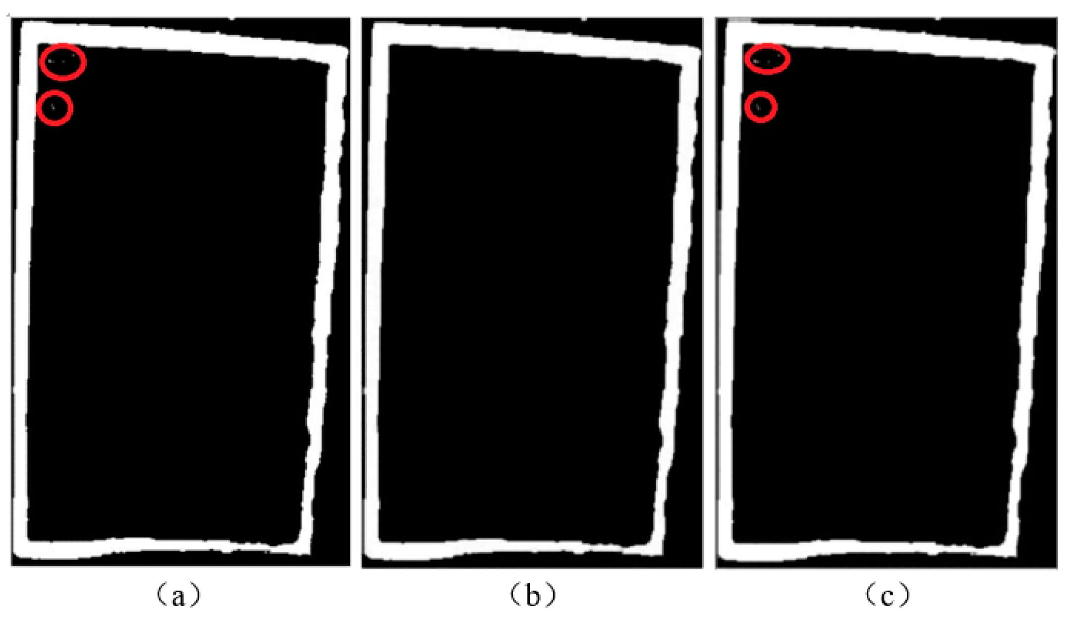
In the morphological processing of images, both open and closed operations consisting of expansion and erosion are able to smooth the surface of the target object, with little effect on the overall size of the target. Figure 18 shows the results of the open and closed operations on the binarized image. The red circle indicates areas with small noise.
The binarized image of the parking space also has the effect of some smaller holes and noise, as shown in (a). After the closed operation processing, there are still some small noises in the red area in (c), and there is no obvious improvement compared with the preprocessing. On the other hand, after the open operation processing, some small noises in the red area in (a) have been eliminated, more clear and accurate information of the parking space is obtained, and the basic outline of the parking space has been extracted, so open operation was ultimately selected for morphological processing.

6. Conclusions

This paper studies an algorithm for car parking space recognition. When stitching and fusing the images after projection transformation, it balanced the brightness of the images by adding equalization adjustment coefficients in order to obtain a brightness-balanced fusion map. The experimental results show that the improved image equalization processing method makes the image brightness look more balanced, and the clarity of the vehicle’s position in the image is significantly improved. The parking spaces were recognized and contour lines extracted based on the YOLOv5 target detection model and OpenCV, respectively. The overall mAP of the parking space recognition model was 96.6%, and the detection speed was 52.3 fps, which is about 57.6 km/h, meeting the requirements of the real-time parking space recognition task during automatic parking. The next research direction will be to locate the corner-point coordinates of the extracted parking spaces in the panoramic surround view map to provide reliable input for the parking control link.

Author Contributions

Conceptualization, X.Z. and W.Z.; methodology, X.Z. and W.Z.; software, W.Z.; validation, X.Z., W.Z. and Y.J.; formal analysis, X.Z. and W.Z.; investigation, W.Z. and Y.J.; writing—original draft preparation, W.Z.; writing—review and editing, X.Z. and W.Z.; supervision, X.Z. and Y.J.; project administration, X.Z.; funding acquisition, X.Z. and Y.J. All authors have read and agreed to the published version of the manuscript.

Funding

The authors would like to acknowledge support from the following projects: Liaoning Province Basic Research Projects of Higher Education Institutions (Grant No. LG202107, LJKZ0239); 2023 Central Guiding Local Science and Technology Development Funds (Grant No. 2023JH6/100100066).

Data Availability Statement

The data used to support the findings of this study are included within the article.

Acknowledgments

The authors sincerely appreciate all financial and technical support.

Conflicts of Interest

The authors declare no conflict of interest.

References

  1. Shin, J.H.; Jun, H.B. A study on smart parking guidance algorithm. Transp. Res. Part C Emerg. Technol. 2014, 44, 299–317. [Google Scholar] [CrossRef]
  2. Zhang, L.; Huang, J.; Li, X.; Xiong, L. Vision-based parking-slot detection: A DCNN-based approach and a large-scale benchmark dataset. IEEE Trans. Image Process. 2018, 27, 5350–5364. [Google Scholar] [CrossRef] [PubMed]
  3. Redmon, J.; Farhadi, A. YOLO9000: Better, faster, stronger. In Proceedings of the IEEE Conference on Computer Vision and Pattern Recognition, Honolulu, HI, USA, 21–26 July 2017; pp. 7263–7271. [Google Scholar]
  4. Jang, C.; Sunwoo, M. Semantic segmentation-based parking space detection with standalone around view monitoring system. Mach. Vis. Appl. 2019, 30, 309–319. [Google Scholar] [CrossRef]
  5. Liu, Z. Design of Parking Spaces Visual Detection and Positioning System of Automatic Parking Based on Deep Learning and OpenCV. Master’s Thesis, Jiang’su University, Zhenjiang, China, 2020. [Google Scholar]
  6. Redmon, J.; Divvala, S.; Girshick, R.; Farhadi, A. You only look once: Unified, real-time object detection. In Proceedings of the IEEE Conference on Computer Vision and Pattern Recognition, Las Vegas, NV, USA, 27–30 June 2016; pp. 779–788. [Google Scholar]
  7. Ren, S.; He, K.; Girshick, R.; Sun, J. Faster R-CNN: Towards Real-Time Object Detection with Region Proposal Networks. IEEE Trans. Pattern Anal. Mach. Intell. 2017, 39, 1137–1149. [Google Scholar] [CrossRef] [PubMed] [Green Version]
  8. Liu, W.; Anguelov, D.; Erhan, D.; Szegedy, C.; Reed, S.; Fu, C.Y.; Berg, A.C. Ssd: Single shot multibox detector. In Proceedings of the Computer Vision–ECCV 2016: 14th European Conference, Amsterdam, The Netherlands, 11–14 October 2016; pp. 21–37. [Google Scholar]
  9. Zhang, Z. A Flexible New Technique for Camera Calibration. IEEE Trans. Pattern Anal. Mach. Intell. 2000, 22, 1330–1334. [Google Scholar] [CrossRef] [Green Version]
  10. Yan, Q.C. Research on Uav Marine Remote Sensing Image Processing and Stitching Algorithm. Master’s Thesis, Yan’shan University, Qinhuangdao, China, 2022. [Google Scholar]
  11. Zhang, J.D.; Liu, T.; Yin, X.L.; Wang, X.; Zhang, K.; Xu, J.; Wang, D. An improved parking space recognition algorithm based on panoramic vision. Multimed. Tools Appl. 2021, 80, 18181–18209. [Google Scholar] [CrossRef]
  12. Dong, X.D.; Yan, S.; Duan, C.Q. A lightweight vehicles detection network model based on YOLOv5. Eng. Appl. Artif. Intell. 2022, 113, 104914. [Google Scholar] [CrossRef]
  13. Wei, C.Y.; Tan, Z.; Qing, Q.X.; Zeng, R.; Wen, G. Fast Helmet and License Plate Detection Based on Lightweight YOLOv5. Sensors 2023, 23, 4335. [Google Scholar] [CrossRef] [PubMed]
  14. Wang, C.Y.; Bochkovskiy, A.; Liao, H.Y.M. YOLOv7: Trainable bag-of-freebies sets new state-of-the-art for real-time object detectors. arXiv 2022, arXiv:2207.02696. [Google Scholar]
  15. Yuan, H.C.; Tao, L. Detection and identification of fish in electronic monitoring data of commercial fishing vessels based on improved Yolov8. J. Dalian Ocean Univ. 2023, 38, 533–542. [Google Scholar]
  16. Meng, X.X. Research on Automatic Parking Method Based on Panoramic Vision. Master’s Thesis, Ji’lin University, Changchun, China, 2021. [Google Scholar]
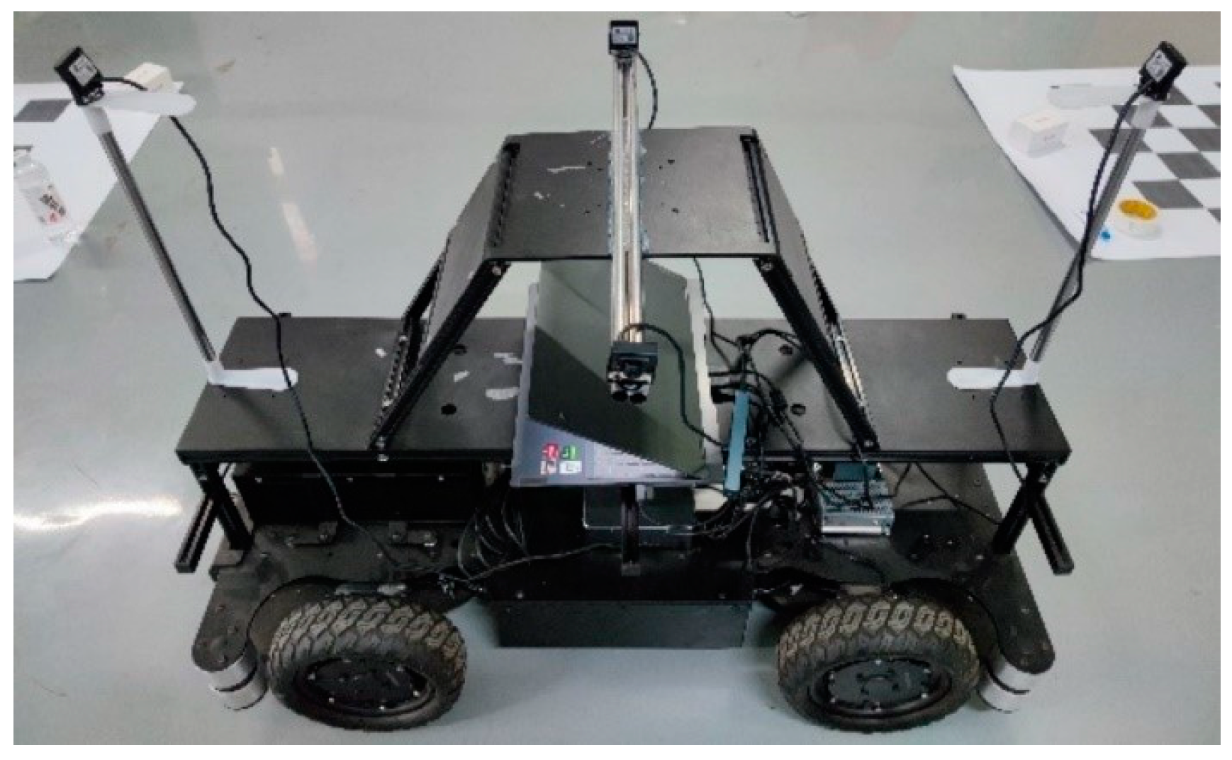
Figure 1. Camera mounting position.
Electronics 12 03374 g001
Figure 2. Original images.
Electronics 12 03374 g002aElectronics 12 03374 g002b
Figure 3. Distortion-corrected images.
Electronics 12 03374 g003
Figure 4. Top view around the body.
Electronics 12 03374 g004
Figure 5. Panoramic splicing diagram.
Electronics 12 03374 g005
Figure 6. Top-view processing results.
Electronics 12 03374 g006
Figure 7. Actual panoramic stitching—top view.
Electronics 12 03374 g007
Figure 8. Fusion graph without equalization.
Electronics 12 03374 g008
Figure 9. Fusion map after equalization.
Electronics 12 03374 g009
Figure 10. Equalization adjustment factor to adjust the brightness of each channel diagram.
Electronics 12 03374 g010
Figure 11. Fusion chart with increased equalization adjustment factor.
Electronics 12 03374 g011
Figure 12. Car parking space dataset statistics.
Electronics 12 03374 g012
Figure 13. Parking space identification effect map.
Electronics 12 03374 g013
Figure 14. Model evaluation results. (a) Training set localization loss function (b) Training set target confidence loss function (c) Training set class loss function (d) Verification set localization loss function (e) Verification set target confidence loss function (f) Verification set class loss function (g) Accuracy curve (h) Recall rate curve (i) [email protected] curve (j) [email protected]:0.95 curve.
Electronics 12 03374 g014
Figure 15. Image grayscale results. (a) Original image (b) Maximum value method (c) Average method (d) Weighted average method.
Electronics 12 03374 g015
Figure 16. Image filtering results. (a) Grayscale map (b) Mean filtering (c) Median filtering (d) Weighted average.
Electronics 12 03374 g016
Figure 17. Adaptive binarization results. (a) Filtered image (b) TRIANGLE adaptive threshold (c) OTSU adaptive threshold.
Electronics 12 03374 g017
Figure 18. Morphological processing results. (a) Binarized images (b) Open operation (c) Closed operation.
Electronics 12 03374 g018
Table 1. Fisheye camera internal parameters.
FrontBackLeftRight
fx1.645 × 1021.592 × 1021.641 × 1021.648 × 102
uo2.996 × 1023.004 × 1023.053 × 1023.085 × 102
fy1.647 × 1021.592 × 1021.642 × 1021.650 × 102
vo2.289 × 1022.436 × 1022.362 × 1022.364 × 102
Table 2. Distortion factor of fisheye cameras.
FrontBackLeftRight
k1−2.450 × 10−21.750 × 10−2−1.608 × 10⁻²−2.504 × 10⁻²
k2−8.646 × 10⁻³−8.381 × 10⁻²−2.815 × 10−21.582 × 10−2
p16.204 × 10−34.853 × 10−23.268 × 10−2−1.061 × 10⁻²
p2−1.727 × 10⁻³−9.363 × 10⁻³−9.159 × 10−31.391 × 10−3
Table 3. Experimental hardware configuration information.
Serial NumberHardwareModel
1Video cardsNVIDIA GeForce RTX 3060 (6G video memory)
2CPUAMD Ryzen7 5800H with Radeon Graphics
3Memory stick 1Samsung DDR4(8G RAM)
4Memory stick 2Micron Technology DDR4(8G memory)
Table 4. Software environment information.
Serial NumberNameVersion Number
1SystemWindows 10
2PyCharmCommunity 2022.2.2
3Python3.8.16
4PyTorch1.12.1
5CUDA11.3
6CUDNN8.4.1.50
Table 5. Performance indicators for training results of several algorithms.
AlgorithmsClassificationPrecision (%)Recall (%)mAP (%)
YOLOv8All92.590.696.8
Vacant91.591.496.7
Occupied93.489.896.9
YOLOv7All90.291.595.2
Vacant89.192.395.8
Occupied91.490.894.7
YOLOv5All93.792.196.6
Vacant93.592.796.8
Occupied93.991.696.4
Disclaimer/Publisher’s Note: The statements, opinions and data contained in all publications are solely those of the individual author(s) and contributor(s) and not of MDPI and/or the editor(s). MDPI and/or the editor(s) disclaim responsibility for any injury to people or property resulting from any ideas, methods, instructions or products referred to in the content.