Abstract
Most well-known supervised dimensionality reduction algorithms suffer from the curse of dimensionality while handling high-dimensional sparse data due to ill-conditioned second-order statistics matrices. They also do not deal with multi-modal data properly since they construct neighborhood graphs that do not discriminate between multi-modal classes of data and single-modal ones. In this paper, a novel method that mitigates the above problems is proposed. In this method, assuming the data is from two classes, they are projected into the low-dimensional space in the first step which removes sparsity from the data and reduces the time complexity of any operation drastically afterwards. These projected data are modeled using a mixture of exponential family distributions for each class, allowing the modeling of multi-modal data. A measure for the similarity between the two projected classes is used as an objective function for constructing an optimization problem, which is then solved using a heuristic search algorithm to find the best separating projection. The conducted experiments show that the proposed method outperforms the rest of the compared algorithms and provides a robust effective solution to the problem of dimensionality reduction even in the presence of multi-modal and sparse data.
1. Introduction
Lately, due to a significant decrease in the cost of deploying sensors and other data collection devices, there has been a surge in the way these devices are used for collecting samples of data. Consequently, there is tremendous redundancy in the stored data and this has been a source of problem for many applications such as data analysis, classification, and clustering. These problems include, but are not limited to, the difficulty of visualization, introducing the curse of dimensionality [1,2], and an excessive need for processing and storage resources. Feature selection techniques [3,4] are a group of methods that are used to remedy this problem; however, dimensionality reduction (DR) methods prove to be a more efficient way of reducing this redundancy while preserving most of the embedded information [5,6,7] since they use a combination of features instead of a subset of them. Such techniques are well studied and researched and are diverse in the approach they adopt to solve the problem. From one general point of view, these algorithms are divided into linear and non-linear types. In case of linear algorithms, a linear transform is used to project the data to the low-dimensional space. These projections are the most popular due to the simplicity of the final transform and the intuitive interpretation of the projection as a weighted sum of the original features and often are based on the second-order statistics of the data [8,9,10,11]. The second-order statistics of data refer to statistical properties that are derived from the covariance matrix of the data, and involve analyzing the relationships between different data features and how they vary together. The covariance matrix captures the interdependencies between variables, providing valuable information about the data’s distribution and structure. In the context of the DR methods, the use of second-order statistics enables an algorithm to preserve important discriminative information and enhance the separability of classes in the reduced feature space. Fisher Discriminant Analysis (FDA) [12], Principal Component Analysis (PCA) [13], Local Fisher Discriminant Analysis (LFDA) [14,15], Factor Analysis (FA) [16], Locality Preserving Projection (LPP) [17], and L1-Norm Fisher Discriminant Analysis (LDA-L1) [18] are some of the well-studied ones among them. In the non-linear category of DR techniques falls any other method that does not use a linear projection for mapping the data into the low-dimensional space. For example, Kernel PCA (KPCA) [19], Maximum Variance Unfolding (MVU) [20], Uniform Manifold Approximation and Projection (UMAP) [21], t-distributed stochastic neighbor embedding (t-SNE) [22], Locally Linear Embedding (LLE) [23], and Kernel-based Within-Class Collaborative Preserving Discriminant Projection (KWCCPDP) [24] are some of the most well known among such methods. These techniques might be a better match to the problem depending on the type of the data and their non-linear nature. From another point of view, DR algorithms can be divided into supervised/unsupervised depending on whether they use available data labels for projecting the data into the low-dimensional space. Of course, the usage of data labels allows supervised DR techniques to capture the hidden structures in the data more effectively.
In this research, we limit our focus to the linear supervised techniques since they are highly efficient and capture the structures in the data very well. However, most of such methods suffer from some weaknesses. For example, some may not be able to handle multi-modal data effectively (for such analysis regarding LPP, see [14]). Also, some (e.g., LFDA and SOLPP) completely fail to produce any results in certain cases due to the sparsity of the data as has been shown in Section 4. While dealing with extremely sparse data, another important issue with many of the conventional algorithms is that the effectiveness of the solution highly depends on the choice of the training data. This is due to the fact that they depend on solving a generalized eigenvalue problem (GEVP), which is more likely to become ill posed when the data are highly sparse.
The above-mentioned weaknesses while dealing with sparse high-dimensional data motivated the design of a DR technique that uses a different approach to tackle the dimensionality reduction problem. This novel DR technique is designed to work best for proportional data with very high dimensions, and specifically designed for classification problems. Its goal is to maximize the separation of data in the new low-dimensional space. Starting with the projection of data classes into the low-dimensional space, it assumes each class of data in this new space has a distribution that is modeled with a mixture of distributions from the exponential family. This mixture allows multi-modal data to be modeled and is one of the advantages of this algorithm. After estimating the parameters of this mixture for each class using the EM algorithm, we use an approximation of the KL (Kullback–Leibler) divergence between the mixtures to estimate their distance. This distance is then used as a measure to be maximized by the algorithm. To this end, one can use an optimization technique to maximize this measure and hence optimize data separation; however, the use of the EM algorithm limits the methods of optimization that can be used efficiently. Specifically, heuristic search methods remain the best option in this case, and we have used GA (genetic algorithm) effectively to solve the problem and find a near-optimal projection for data separation. As mentioned above, the proposed technique uses distributions from the exponential family. The choice of the distribution depends on the type of the data and the hidden structures, e.g., the structure of the covariance matrix. Nevertheless, as has been shown in the literature, some distributions can model proportional data effectively [25,26,27,28,29,30,31] and we have used such distributions. It is important to note that any desirable subset of distributions from the set of exponential family distributions can be used in the proposed method. In general, our contributions is this paper can be summarized as follows:
- Proposing a novel supervised dimensionality reduction method that addresses the curse of dimensionality in high-dimensional sparse proportional data by projecting data into a low-dimensional space, mitigating sparsity significantly.
- Introducing a unique approach to handle multi-modal data by modeling the projected data using a mixture of exponential family distributions for each class, allowing for effective discrimination between multi-modal and single-modal classes.
- Formulating a closed form for the similarity between projected classes using KL-Divergence and employing a heuristic search algorithm to optimize the separation of classes, resulting in a robust and efficient solution to the problem of dimensionality reduction, outperforming other compared algorithms in diverse experimental settings.
The remainder of this work is structured as follows. In Section 2, some conventional techniques of DR are introduced which are used in the experiments for comparison purposes to show the effectiveness of the designed method. The problem is formulated in detail in Section 3. In Section 4, different datasets are used to test the performance of the proposed technique. Finally, we draw our conclusion and present some final words in Section 5.
2. Related Works
As has been mentioned before, conventional linear DR methods, despite all their differences, use the second-order statistics of data to formulate and solve a GEVP. In this section, we will briefly discuss some of the well-known supervised linear DR techniques that are used in the literature, and will use them to assess the performance of our algorithm later in Section 4.
Supervised Locality Preserving Projection (SLPP) [32] is an extension of the Locality Preserving Projection (LPP) method and is adapted to use the labels of the data. In LPP, first, a matrix A with elements is defined to reflect the neighborhood of the data, and, based on this matrix, a transform T is defined as follows.
where M is the number of data points, N and K are the original and target dimensions respectively, and denotes a data point. Moreover, the elements of D are
Solving the bellow GEVP, one can find the transform T.
By choosing the K eigenvectors corresponding to the K smallest eigenvalues of the above GEVP, the transform T will reduce the dimensionality of the data to K.
LPP and its derivatives suffer from several problems, including overfitting, sensitivity to noise, and disconnectivity of the neighborhood graph. In [33], the authors introduce Supervised Optimal Locality Preserving Projection (SOLPP) to tackle these problems. This has been accomplished by defining a discriminating similarity matrix between data points called W. The following constrained optimization problem is then formulated, where and indicates the i-th row of T.
By solving this problem using an iterative method, the optimal projection T can be evaluated.
Locality Sensitive Discriminant Analysis (LSDA) [34] is based on two connectivity graphs, corresponding to inter-class and intra-class distances. By incurring heavy penalty for neighboring points from the same class being mapped far from each other, or nearby points from different classes being mapped close to each other, the authors formulate an optimization problem and find an optimal projection.
Fisher Discriminant Analysis (FDA) starts by formulating the inter-class and intra-class scatter matrices as follows:
where
Here, and are the label of the sample and the number of samples in class l, respectively. Solving the following optimization problem, one can arrive at the optimal projection of FDA.
The optimal transform T is actually formed by the K eigenvectors corresponding to the K smallest eigenvalues of the following GEVP.
The authors in [14], on the other hand, use an affinity matrix similar to LPP to rebuild the scatter matrices and as below.
Replacing these matrices with those of Equations (6) and (7), a new GEVP can be solved to find the optimal projection corresponding to LFDA.
Finally, in [18], the authors introduce a new variant of LDA by replacing the L2 norm with the L1 norm. This will make the algorithm more robust to outliers and sparsity; however, the resulting problem is non-convex and therefore an iterative method must be used to find the optimal projection.
All the above-mentioned methods of DR have been proved to be efficient in the literature. Nevertheless, they fail to effectively solve the problem of dimensionality reduction in some cases. For instance, they mostly rely on the second-order statistics of data and solving a GEVP. For very high-dimensional data (and specifically for the case of proportional data), however, the sparsity of the data matrix results in near-singular correlation matrices that cause the GEVP to be ill posed and not result in an optimal solution. Moreover, the above methods majorly rely on the construction of a neighborhood graph that sometimes becomes disconnected and affects the solution of the GEVP. Multi-modal data representation is another important task in which the above methods often fail [14]. Note that in all of the above methods, the algorithm has to manipulate very large-size matrices, and, for example, invert large sparse matrices, which is inefficient and of the order of in terms of complexity. Therefore, the complexity of the problem can grow rapidly by the number of features. Finally, note that none of the mentioned algorithms are designed for proportional data specifically and therefore the projected data may not respect the proportionality condition.
The above-mentioned problems with the current supervised linear DR methods motivate us to introduce EXMMP. This algorithm is designed specifically as a pre-processing step in classification problems. Therefore, easy separation of data classes is of utter importance in this algorithm. Since we start with mapping the data using a projection matrix to the low-dimensional space, at this very first step, the problem of sparsity is resolved to a good extent. The complexity of the algorithm, on the other hand, is not affected heavily by the number of original features or the number of available samples. Note that the heuristic search for the optimal projection embeds a property for the projection that guarantees the proportionality of the mapped data, and therefore, unlike the conventional methods, maps proportional data to a corpus of proportional data. As the final advantage, the usage of mixture models allows the algorithm to model multi-modal data, where the rest of the algorithms are unable to do so and fail to capture this property.
3. Proposed Method
3.1. Problem Statement
In this section, we will state the problem and formulate our method, which resolves the issue of the sparsity of the data that hinders other algorithms in reducing the dimensionality of data properly. We use a mixture of distributions from the exponential family along with an estimation of the KL-Divergence between two mixtures—a similarity measure to optimize the separability of classes.
Consider a set of proportional data containing M samples of N dimensions. Let us represent each sample with where
and . Also, is the j-th element of the i-th sample . To facilitate the manipulation of this data set, the matrix X is formed by accumulating s as its columns. The proposed algorithm maps this corpus of data from the N-dimensional space to a smaller K-dimensional space where . Representing this projection with P, the new K-dimensional data set Y can be found as follows.
Note that after the projection, columns of Y represent the corresponding data samples in the original data matrix. Denote the elements of P by , where and . Moreover, to maintain the proportionality of the projected samples, we assume the following property for P (which is both necessary and sufficient for the projected data to be proportional [30]):
3.2. Class Distribution Estimation
In this step, we assume that the projected data of each class are generated using a specific distribution. This distribution will then be used, along with its counterpart from the other class, to maximize data separation in the low-dimensional space. Furthermore, we are going to make the assumption that this generating distribution is one of the distributions from the exponential family and has a support on a simplex. These two assumptions are crucial since the former facilitates the derivation of the results and the latter conforms to the fact that the data are proportional [25]. Note that henceforward, it is assumed that each class of (projected) data is modeled with a mixture of a specific distribution. This assumption is also critical for the capacity of the algorithm for modeling multi-modal data. In the following, the EM (Expectation–Maximization) algorithm is used for estimating the parameters of such mixture model.
Representing the projected samples by , their distribution can be written as
where , ; the vertical vector contains the corresponding parameters of the j-th component; the matrix , of which the columns are s, represents the complete set of the parameters of the mixture; and the number of components in the mixture is represented by Q. Also, note that the prior s conform to the following:
Now, assuming two training sample sets and are chosen from two classes of data such that and , the likelihood of the data given the parameter is as follows
where samples are assumed to be i.i.d., is the i-th sample from class and the matrix is constructed by a column-wise population of all the class samples. Now, using the EM algorithm and latent variables , which are indices for mixture assignment, one can find such that this likelihood is maximized. First, the mixing weights are estimated from the equation
where t is the iteration number and is the expected value of .
In the next step, to maximize the log likelihood, must be evaluated by solving the below set of equations
where , is the number of the parameters of the distribution, , and is the k-th element of .
Let us assume the following distribution from the exponential family:
where the base measure (a real-valued function) and sufficient statistics (a vector-valued functions) are independent of the distribution parameter, (the natural parameter) is a vector-valued function of , and (the log partition) is a real-valued function of . Using this distribution in the EM algorithm, the maximization step yields the following system of equations for and :
where indicates the k-th element of and is the number of elements in the natural parameter. Simplifying the above system results in a set of equations
where is the k-th element of the sufficient statistics function . Due to the non-linearity of the above system, no closed-form solution is available to find the maximizing parameters. Therefore, some type of numerical method is required to find the result. In this paper, the Newton–Raphson (NR) algorithm, which is one of the most well-known methods, has been used to find the parameters of the distribution. This method uses the Jacobian of the system which is the Hessian matrix of the original system, and hence will be called H for and . This matrix only depends on the log partition function and is evaluated below.
Note that since is independent of for , the resulting Jacobian matrix will be block diagonal which is a significant advantage since inverting this matrix will be of order of complexity instead of (assuming cubic complexity for inverting a matrix).
3.3. Measuring Inter-Class Distance
To facilitate separation of the data, we develop a measure of distance between the two projected classes. One of the most well-known measures of distance between distributions is the KL-Divergence [35], and it has been used in this section. Finding a closed form for evaluating the KL-Divergence between two mixtures of distributions is not trivial. To do so, we follow a method similar to the one in [36]. Assuming two mixtures and consisting of and components, respectively, we start with the following equations.
Based on the definition of KL-Divergence, one arrives at
The first term of the above equation can be expanded as follows.
A maximum lower bound for the left side of the above statement can be found using Jensen’s inequality, adjusting the introduced parameters in the equation below.
Note that for the above to be true, the following condition must hold.
To find the proper parameters, we form the following cost function:
for which the KKT (Karush–Kuhn–Tucker) conditions [37] are as below.
The solution to this optimization problem is
where we define the function as
Similarly, a maximized lower bound can be found for the second term of Equation (25), which is as below.
Using the resulting two maximized lower bounds and noting that
a closed-form approximation can be found for the KL-Divergence of two mixtures of distributions.
Note that this allows the KL-Divergence of two mixtures to be approximated in a closed form using the KL-Divergence of the two corresponding single distributions.
The KL-Divergence of two distributions and from the exponential family with parameters and , respectively, is as below.
Note that denotes the expected value with respect to . To simplify the first term on the right-hand side of Equation (36), we plug Equation (20) and obtain
Similarly, for the second term,
And therefore, the closed form of the KL-Divergence will reduce to
After this final step, a closed-form approximation for the KL-Divergence of two mixtures of distributions can be obtained by using Equation (39) in Equation (35). Also, note that in this work we have used an approximation of the symmetric form of the KL-Divergence, namely, J-Divergence, which is formulated as follows.
3.4. Maximizing Class Distance
To find the projection that maximizes the class distance between two projected classes, an optimization problem must be formulated. In the case of high-dimensional data, this results in solving for a significantly large number of parameters of the projection matrix, namely . Considering that estimating the parameters of the two mixtures of distributions is performed using the EM algorithm, which is iterative, using conventional optimization techniques such as Gradient Descent (GD) is not practical in terms of complexity. Also, note that the fitness function has many local minima and, hence, the GD method is not suitable for this matter. Therefore, considering the nature of the problem, a heuristic search algorithm proves to be a proper method. In this paper, we use genetic algorithm (GA) along with the above-developed measure of distance as the fitness function. The initial population in the GA is a set of random matrices which conform to Equation (14). In each iteration, the data from both classes are projected to the low-dimensional space using one of the members of the current population, and the mixture parameters for each class of data are estimated and, then, used in Equation (40) to evaluate the fitness of the projecting matrix. This value is then used in the GA to find the optimum projection. Algorithm 1 briefly describes this process in the form of pseudo-code.
| Algorithm 1 Summary of the proposed algorithm |
|
4. Experimental Results
4.1. Test Scenarios
To prove the efficacy of the proposed technique, it is compared with several supervised linear DR methods in this section. As mentioned, EXPMMP uses distributions from the exponential family to model the data. However, distributions with support on the simplex are better suited for proportional/compositional data. In [38], Aitchison shows that an invertible function, specifically the log-ratio transformation, can be used to convert the support of any distribution to a simplex. For the experiments in this section, we used three distributions which are defined on a simplex: Dirichlet, Generalized Dirichlet, and Beta-Liouville. Moreover, we used the Additive Logistic Normal (ALN) distribution for our tests, which uses the above-mentioned log-ratio function along with the normal distribution. For all the performed experiments, a corpus of labeled data from two classes was mapped to a low-dimensional space using all the algorithms, followed by a Decision Tree (DT) classifier for classification. The choice of classes was made either randomly or based on the number of samples of that class in the dataset, where the classes with a high number of samples were chosen for reliable results. For the proposed method, we divided the data into training, validation, and testing sub-sets. This allowed us to perform the algorithm using different distributions and, after the training phase, choose the projection corresponding to the distribution that yielded the best classification accuracy on the validation sub-set. Note that the reported values in the tables of this section are all from test sub-set and each test was repeated 5 times while each repetition used a fivefold cross-validation method. The reported values in the tables are average accuracies and their corresponding standard deviation. Also, note that some algorithms are not present in the tables, which shows they have failed to produce any meaningful result.
Experiment 1: For the first experiment, the 20-Newsgroups dataset was used in the form of a bag-of-words model. This dataset contains 20,000 samples of text from 20 different classes and originally has 61,189 words. We chose two classes of data, namely atheism and forsale, and projected these classes into a low-dimensional space after reducing their features to 1000 by removing stop words and low-frequency features. Table 1 represents the resulting accuracies for the compared and proposed algorithms. Note that, the test was run also on SOLPP and LFDA, which did not yield any result since these algorithms could not solve the eigenvalue problem due to the sparsity of the data. Also, SLPP and LSDA reported very high deviation values in the tests, which is due to the fact that depending on the training sub-set, they may fail to solve the eigenvalue problem, again, because of the sparsity of the representing matrix. On the other hand, EXPMMP consistently reports a high accuracy of classification with a low value of standard deviation for different tests. To contextualize these results in relation to our objectives, we aimed to address the challenge of high-dimensional data classification while considering the sparsity inherent in the data. Our experiments demonstrate that EXPMMP successfully tackles this challenge, showcasing its potential as a promising solution for handling high-dimensional sparse data and achieving improved classification accuracy.

Table 1.
Classification accuracy (%) of 20-newsgroups dataset for different target dimensions K, and 1000 original features. Boldface shows the best result.
Experiment 2: To test the proposed algorithm for a different application, we used the Caltech-256 dataset, which consists of different samples of 256 objects. Some sample images from this dataset are presented in Figure 1. In this experiment, two image categories were chosen and their SIFT features were extracted. This set of features was used to construct a VBoW (Visual Bag of Words) using a dictionary of 750 words. The proposed method was then run on this binary classification problem along with the other compared algorithms with a target dimension of 3. Table 2 shows the results of this classification. As has been mentioned before, a DT was used to classify the reduced-dimension data and the mean and standard deviation of the resulting accuracies from all the tests have been reported. Note that the use of a low target dimension of 3 allows for a meaningful reduction in the feature space, effectively enhancing computational efficiency while preserving essential discriminative information. This aligns with our goal of developing an efficient yet accurate approach for high-dimensional data classification.
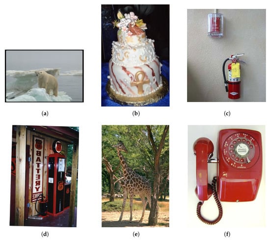
Figure 1.
Sample images from different categories (classes) in Caltech-256 dataset.
Table 2.
Classification accuracy (%) of Caltech-256 dataset for unimodal data, . Boldface shows best result.
Note that the SOLPP and LFDA methods did not yield any results due to the sparsity of the data. Moreover, the proposed method performs better than the rest of the algorithms, consistently, in terms of both the average and standard deviation of accuracies, which shows that our proposed method is effective on diverse types of data.
Experiment 3: This experiment tested the proposed method using a different image dataset called Linnaeus-5 [39]. This dataset consists of images of five subjects (Berry, Bird, Dog, Flower, Other) each containing 1600 images. Following the same methodology used in the previous image classification experiment, we constructed a Visual Bag of Words (VBoW) representation with a dictionary size of 750 words. The extracted features were then employed for binary classification using the proposed method and several state-of-the-art algorithms as comparators. The results of this classification experiment are summarized in Table 3. Notably, the proposed method consistently outperforms the compared algorithms in terms of classification accuracy across all categories. This noteworthy improvement in accuracy highlights the effectiveness and robustness of our proposed approach, even when applied to a different and challenging image dataset like Linnaeus-5. By achieving superior accuracy consistently, our method showcases its potential for addressing real-world image classification tasks with diverse subject categories. The reliable performance of our algorithm on the Linnaeus-5 dataset reaffirms its generalizability and underscores its relevance in handling high-dimensional image data across various domains.
Table 3.
Classification accuracy (%) of Linnaeus-5 dataset for unimodal data, . Boldface shows best result.
Experiment 4: In this experiment we, again, used the 20-Newsgroups dataset, although in a different setup. In this case, we fixed the target dimension to 3 while we tested different pairs of classes against each other. The preprocessing step left 1000 original features, which were reduced to 3 using all the algorithms. Table 4 presents the results of this pairwise classification test. As expected, the sparsity of the data posed challenges for certain algorithms. Specifically, SOLPP and LFDA encountered difficulties in finding a suitable low-dimensional representation for the data in this particular setup, leading to suboptimal performance or failure to provide meaningful results. In contrast, our proposed method consistently outperformed the compared algorithms in all cases, achieving superior classification accuracy for the pairwise tests. The ability of our method to handle the fixed target dimension of 3 while maintaining competitive performance underscores its adaptability and robustness in handling diverse experimental conditions. The outcomes of this experiment provide valuable insights into the strengths and limitations of the algorithms tested. The difficulties faced by SOLPP and LFDA emphasize the importance of choosing an appropriate method that aligns with the specific experimental setup and dataset characteristics (in this case, sparse compositional data). Moreover, the consistently better performance of our proposed method confirms its efficacy in capturing relevant discriminative information and effectively representing data in a low-dimensional space, even under challenging conditions.
Table 4.
Classification accuracy (%) of 20-newsgroups dataset for unimodal data, . Boldface shows best result.
Experiment 5: In this experiment, the ImageNet dataset was used to compare the proposed method with the rest of the algorithms. This dataset is composed of more than 20,000 categories with a different number of images in each category. Similar to Experiment 2, we chose two image categories in each test and constructed a VBoW with a 750-word dictionary. Then, we reduced the dimension of the data to 3 and used DT to classify the images. The results of the tests are presented in Table 5. Notably, we observed that our proposed method consistently achieved competitive results compared to the other algorithms across different category pairings. The ability of our method to maintain its performance on the vast and diverse ImageNet dataset underscores its potential as a robust and versatile approach for large-scale sparse image datasets. The ImageNet dataset poses significant challenges due to its diversity, with categories exhibiting varying image quantities and unique visual characteristics. Despite these complexities, our proposed method showed its capacity to capture meaningful discriminative information effectively, even when the representation of the images were highly sparse. Our objective for this experiment was twofold: firstly, to assess the performance of the proposed method on a widely recognized and complex image dataset, and secondly, to highlight its adaptability to highly sparse proportional data even when the target dimension is as low as 3.
Table 5.
Classification accuracy (%) of ImageNet dataset for unimodal data, . Boldface shows best result.
Experiment 6: In this experiment, we used an image dataset known as Food-101 which contains images from 101 types of dishes. Similar to the previous experiments, we chose pairs of classes, constructed a VBoW for each pair using a 750-word vocabulary and SIFT features, and reduced the dimensionality to 3. The data were then classified and the test was repeated, and the mean and standard deviation of the accuracies were evaluated. Table 6 presents the results of this test. As observed, our proposed method consistently outperformed the compared algorithms across all class pairings. The ability of our method to maintain its superiority on the Food-101 dataset with its diverse visual characteristics underscores its effectiveness in image classification tasks under significantly sparse conditions. Notably, certain algorithms, such as SOLPP and LFDA, encountered challenges in producing meaningful results on this dataset. The difficulties faced by these algorithms highlight the importance of choosing appropriate methods that can handle the sparsity of the dataset. The consistently superior results achieved by our proposed method reaffirm its potential as a powerful tool for dimensionality reduction of proportional sparse data.
Table 6.
Classification accuracy (%) of Food-101 dataset for unimodal data, . Boldface shows best result.
Example 7: In this test, we investigated the capacity of the introduced method for the case of multi-modal data. The previously used dataset, Food-101, was used in this case. After choosing three classes of data, two of them were combined as one multi-modal class and used for classification against the third. Similar to the previous tests, after constructing a VBoW model and reducing the dimensionality to 3, the samples were classified using a DT classifier. Table 7 presents the results of this multi-modal data test. Note that our proposed method consistently outperformed the compared algorithms in terms of both robustness and accuracy. This significant performance gain further supports the efficacy and adaptability of our approach, even when handling multi-modal data with diverse classes. The successful classification results achieved by our method on the multi-modal dataset highlight its potential in various real-world scenarios, where the dimensionality of sparse proportional data from different modalities need to be reduced to be effectively utilized for classification tasks. The ability of our method to consistently outperform the rest of the algorithms in this multi-modal data scenario further strengthens its position as a versatile and reliable solution for dimensionality reduction of highly sparse proportional data.
Table 7.
Classification accuracy (%) of Food-101 dataset for multi-modal data, . Boldface shows best result.
4.2. Complexity Analysis
In terms of performance and computational complexity, the proposed method solves a major problem in the compared algorithms. Most of the linear DR methods in the literature formulate and solve a GEVP. In cases of extremely high-dimensional data though, this GEVP cannot be solved efficiently. Moreover, often, solving this problem involves manipulating sparse high-dimensional matrices that result in near-singular matrices. The proposed method takes a different approach to resolve this issue. The original data are first projected into the new low-dimensional space, and, therefore, all the calculations are performed in the low-dimensional space, which avoids all the problems caused by the sparsity and high dimensionality of the data. In fact, the main reason SOLPP and LFDA did not yield any results in our experiments is that the data were extremely sparse. Also note that the proposed algorithm has the capacity to be parallelized easily, since the evaluation of the fitness function in the GA is independent for different members. This can be achieved even in the case of one processing unit leveraging vector calculations in software packages. In fact, the most intensive calculation in our proposed method is the matrix multiplication of the candidate projections with the data. This can be performed highly efficiently by concatenating all the projections, multiplying this matrix by the data, and then disassembling the resulting projected data. Such matrix multiplications are often performed very efficiently, with minimal time complexity in the current software libraries.
Moreover, the proposed method is significantly lighter in terms of resource usage since it (unlike the rest of the methods) does not need to invert any high-dimensional matrices that are of the order , and, due to the fact that it only uses some statistics of the data (compared to the rest of the algorithms which have to build a neighborhood matrix of size ), it needs much fewer resources, which becomes very important in the case that there are a large number of samples or the algorithm is running on low-power, low-resource devices. In general, the time complexity of solving the GEVP using dense linear algebra techniques is typically on the order of , specifically for some software libraries, where c is a constant depending on the specific implementation and machine architecture. If the matrix is sparse, specialized algorithms based on iterative methods are often used to solve the GEVP more efficiently. However, the time complexity of these sparse eigenvalue solvers is still on the order of to , where k is the number of desired eigenpairs (eigenvectors and eigenvalues), which, considering the large dimensionality of the data, is a significantly time-consuming process. Finally, the choice of the distributions used in the algorithm is affected by several properties of the data. In case there is no information about the underlying distribution of the data, the covariance matrix structure and the number of parameters of each distribution (in relation to the number of training samples) are good guides for choosing the possible candidate distributions.
5. Conclusions
High-dimensional sparse data are encountered more and more due to the low cost and ease of acquiring data, and several problems, including but not limited to the curse of dimensionality and resource usage, are associated with this type of data. In the present work, we have introduced an algorithm of supervised linear dimensionality reduction that remedies some of the problems of the conventional DR techniques in this context. The method has been tested against some of the well-known dimensionality reduction techniques and its superiority was demonstrated. Considering that the curse of dimensionality is a major problem while manipulating sparse data, our proposed method solves this problem effectively. The experiments show that EXMMP is, unlike the rest of the methods, robust in all cases of sparse data and yields better accuracies. It also can handle multi-modal data due to the fact that it models the data using a mixture of distributions, while the rest of the algorithms fail to do so. Moreover, the algorithm is scalable since increasing the number of features and samples have minimum effect on the complexity. Note that this increase only affects the first step of the algorithm, which is the projection into the low-dimensional space in the form of a matrix multiplication, while in the rest of the methods, it is carried along in the algorithm to the last step. Our contributions are briefly summarized below:
- Proposing a novel supervised DR method that addresses the sparsity of the data effectively and efficiently.
- Introducing a unique approach to handle multi-modal data by modeling the projected data using a mixture of exponential family distributions.
- Formulating a closed form of KL-Divergence between the mixtures as a measure of separability.
Considering the above advantages, EXMMP is an effective tool in solving problems related to sparse high-dimensional data. Finally, as the next step in the further development of the algorithm, one can consider using other measures of distance between mixtures of distributions which yields better data separation. Also, the method can benefit from using a better approximation for the closed form of the KL-Divergence.
Author Contributions
Conceptualization, W.M. and N.B.; methodology, W.M.; software, W.M.; validation, W.M. and N.B.; data curation, W.M.; writing—original draft preparation, W.M.; writing—review and editing, W.M. and N.B.; visualization, W.M.; supervision, N.B.; funding acquisition, N.B. All authors have read and agreed to the published version of the manuscript.
Funding
This research was funded by Natural Sciences and Engineering Research Council of Canada (NSERC) under Grants to N. Bouguila (NSERC RGPIN/6656-2017).
Data Availability Statement
The datasets used for our experiments are publically available in the following links:
- 20-newsgroups: UCI Machine Learning Repository https://archive.ics.uci.edu/datasets (accessed on 24 June 2023).
- Caltech-256: Caltech Data by Caltech Library https://data.caltech.edu/records/nyy15-4j048 (accessed on 24 June 2023).
- Linnaeus-5: http://chaladze.com http://chaladze.com/l5/ (accessed on 24 June 2023).
- ImageNet: https://www.image-net.org https://www.image-net.org/ (accessed on 24 June 2023).
- Food101:ETH Zurich https://data.vision.ee.ethz.ch/cvl/datasets_extra/food-101/ (accessed on 24 June 2023).
Conflicts of Interest
The authors declare no conflict of interest.
References
- Donoho, D.L. High-dimensional data analysis: The curses and blessings of dimensionality. AMS Math Chall. Lect. 2000, 1, 32. [Google Scholar]
- Pedagadi, S.; Orwell, J.; Velastin, S.; Boghossian, B. Local fisher discriminant analysis for pedestrian re-identification. In Proceedings of the 2013 IEEE Computer Society Conference on Computer Vision and Pattern Recognition, Washington, DC, USA, 23–28 June 2013; pp. 3318–3325. [Google Scholar]
- Chandrashekar, G.; Sahin, F. A survey on feature selection methods. Comput. Electr. Eng. 2014, 40, 16–28. [Google Scholar] [CrossRef]
- Liu, K.; Fu, Y.; Wu, L.; Li, X.; Aggarwal, C.; Xiong, H. Automated Feature Selection: A Reinforcement Learning Perspective. IEEE Trans. Knowl. Data Eng. 2023, 35, 2272–2284. [Google Scholar] [CrossRef]
- Bruni, V.; Cardinali, M.L.; Vitulano, D. A Short Review on Minimum Description Length: An Application to Dimension Reduction in PCA. Entropy 2022, 24, 269. [Google Scholar] [CrossRef] [PubMed]
- Abdulhammed, R.; Musafer, H.; Alessa, A.; Faezipour, M.; Abuzneid, A. Features Dimensionality Reduction Approaches for Machine Learning Based Network Intrusion Detection. Electronics 2019, 8, 322. [Google Scholar] [CrossRef]
- Chao, G.; Luo, Y.; Ding, W. Recent Advances in Supervised Dimension Reduction: A Survey. Mach. Learn. Knowl. Extr. 2019, 1, 341–358. [Google Scholar] [CrossRef]
- Cunningham, J.P.; Ghahramani, Z. Linear dimensionality reduction: Survey, insights, and generalizations. J. Mach. Learn. Res. 2015, 16, 2859–2900. [Google Scholar]
- Zhuo, L.; Cheng, B.; Zhang, J. A comparative study of dimensionality reduction methods for large-scale image retrieval. Neurocomputing 2014, 141, 202–210. [Google Scholar] [CrossRef]
- Lu, H.; Plataniotis, K.N.; Venetsanopoulos, A.N. A survey of multilinear subspace learning for tensor data. Pattern Recognit. 2011, 44, 1540–1551. [Google Scholar] [CrossRef]
- Jiang, X. Linear subspace learning-based dimensionality reduction. IEEE Signal Process. Mag. 2011, 28, 16–26. [Google Scholar] [CrossRef]
- Fisher, R.A. The use of multiple measurements in taxonomic problems. Ann. Eugen. 1936, 7, 179–188. [Google Scholar] [CrossRef]
- Jolliffe, I.T. Principal Component Analysis. Encycl. Stat. Behav. Sci. 2002, 30, 487. [Google Scholar]
- Sugiyama, M. Dimensionality reduction of multimodal labeled data by local fisher discriminant analysis. J. Mach. Learn. Res. 2007, 8, 1027–1061. [Google Scholar]
- Sugiyama, M.; Idé, T.; Nakajima, S.; Sese, J. Semi-supervised local Fisher discriminant analysis for dimensionality reduction. J. Mach. Learn. 2010, 78, 35–61. [Google Scholar] [CrossRef]
- Bartholomew, D.J. The foundations of factor analysis. Biometrika 1984, 71, 221–232. [Google Scholar] [CrossRef]
- He, X.; Niyogi, P. Locality preserving projections. Neural Inf. Process. Syst. 2004, 16, 153. [Google Scholar]
- Wang, H.; Lu, X.; Hu, Z.; Zheng, W. Fisher Discriminant Analysis With L1-Norm. IEEE Trans. Cybern. 2014, 44, 828–842. [Google Scholar] [CrossRef]
- Schölkopf, B.; Smola, A.; Müller, K.R. Nonlinear component analysis as a kernel eigenvalue problem. Neural Comput. 1998, 10, 1299–1319. [Google Scholar] [CrossRef]
- Weinberger, K.; Saul, L. An introduction to nonlinear dimensionality reduction by maximum variance unfolding. In Proceedings of the 2006 Twenty First National Conference on Artificial Intelligence, Boston, MA, USA, 16–20 July 2006; pp. 1683–1686. [Google Scholar]
- McInnes, L.; Healy, J.; Melville, J. UMAP: Uniform Manifold Approximation and Projection for Dimension Reduction. arXiv 2020, arXiv:1802.03426. [Google Scholar]
- van der Maaten, L.; Hinton, G. Visualizing Data using t-SNE. J. Mach. Learn. Res. 2008, 9, 2579–2605. [Google Scholar]
- Roweis, S.T.; Saul, L.K. Nonlinear dimensionality reduction by locally linear embedding. Science 2000, 290, 2323–2326. [Google Scholar] [CrossRef] [PubMed]
- Hu, H.; Feng, D.; Yang, F. A Promising Nonlinear Dimensionality Reduction Method: Kernel-Based within Class Collaborative Preserving Discriminant Projection. IEEE Signal Process. Lett. 2020, 27, 2034–2038. [Google Scholar] [CrossRef]
- Bouguila, N.; Ziou, D. A dirichlet process mixture of generalized dirichlet distributions for proportional data modeling. IEEE Trans. Neural Netw. 2010, 21, 107–122. [Google Scholar] [CrossRef] [PubMed]
- Fan, W.; Bouguila, N. Learning finite Beta-Liouville mixture models via variational Bayes for proportional data clustering. In Proceedings of the 2013 IJCAI International Joint Conference on Artificial Intelligence, Beijing, China, 3–9 August 2013; pp. 1323–1329. [Google Scholar]
- Epaillard, E.; Bouguila, N. Proportional data modeling with hidden Markov models based on generalized Dirichlet and Beta-Liouville mixtures applied to anomaly detection in public areas. Pattern Recognit. 2016, 55, 125–136. [Google Scholar] [CrossRef]
- Masoudimansour, W.; Bouguila, N. Dimensionality reduction of proportional data through data separation using dirichlet distribution. Image Anal. Recognit. 2015, 9164, 141–149. [Google Scholar]
- Blei, D.M.; Ng, A.Y.; Jordan, M.I. Latent Dirichlet allocation. Mach. Learn. Res. 2012, 3, 993–1022. [Google Scholar]
- Wang, H.Y.; Yang, Q.; Qin, H.; Zha, H. Dirichlet component analysis: Feature extraction for compositional data. In Proceedings of the 2008 25th International Conference on Machine Learning, Helsinki, Finland, 5–9 July 2008; pp. 1128–1135. [Google Scholar]
- Epaillard, E.; Bouguila, N. Hidden Markov models based on generalized dirichlet mixtures for proportional data modeling. Lect. Notes Comput. Sci. 2014, 8774, 71–82. [Google Scholar]
- Shen, Z.H.; Pan, Y.H.; Wang, S.T. A supervised locality preserving projection algorithm for dimensionality reduction. Pattern Recognit. Artif. Intell. 2008, 21, 233–239. [Google Scholar]
- Wong, W.K.; Zhao, H.T. Supervised optimal locality preserving projection. Pattern Recognit. 2012, 45, 186–197. [Google Scholar] [CrossRef]
- Cai, D.; He, X.; Zhou, K.; Han, J.; Bao, H. Locality sensitive discriminant analysis. In Proceedings of the 20th International Joint Conference on Artifical Intelligence, Hyderabad, India, 6–12 January 2007; pp. 708–713. [Google Scholar]
- Kullback, S. Information Theory and Statistics; Dover Publications: Mineola, NY, USA, 1997. [Google Scholar]
- Hershey, J.R.; Olsen, P.A. Approximating the Kullback-Leibler divergence between Gaussian mixture models. Acoust. Speech Signal Process. 2007, 4, 317–320. [Google Scholar]
- Kuhn, H.W.; Tucker, A.W. Nonlinear programming. In Second Berkeley Symposium on Mathematical Statistics and Probability; Springer: Basel, Switzerland, 1951; pp. 481–492. [Google Scholar]
- Aitchison, J. The Statistical Analysis of Compositional Data; Monographs on Statistics and Applied Probability; Chapman and Hall: Boca Raton, FL, USA, 1986. [Google Scholar]
- Chaladze, G.; Kalatozishvili, L. Linnaeus 5 Dataset for Machine Learning. 2017. Available online: http://chaladze.com/l5/ (accessed on 24 June 2023).
Disclaimer/Publisher’s Note: The statements, opinions and data contained in all publications are solely those of the individual author(s) and contributor(s) and not of MDPI and/or the editor(s). MDPI and/or the editor(s) disclaim responsibility for any injury to people or property resulting from any ideas, methods, instructions or products referred to in the content. |
© 2023 by the authors. Licensee MDPI, Basel, Switzerland. This article is an open access article distributed under the terms and conditions of the Creative Commons Attribution (CC BY) license (https://creativecommons.org/licenses/by/4.0/).