Maintain a Better Balance between Performance and Cost for Image Captioning by a Size-Adjustable Convolutional Module

Abstract

Image captioning is a challenging AI problem that connects computer vision and natural language processing. Many deep learning (DL) models have been proposed in the literature for solving this problem. So far, the primary concern of image captioning has been focused on increasing the accuracy of generating human-style sentences for describing given images. As a result, state-of-the-art (SOTA) models are often too expensive to be implemented in computationally weak devices. In contrast, the primary concern of this paper is to maintain a balance between performance and cost. For this purpose, we propose using a DL model pre-trained for object detection to encode the given image so that features of various objects can be extracted simultaneously. We also propose adding a size-adjustable convolutional module (SACM) before decoding the features into sentences. The experimental results show that the model with the properly adjusted SACM could reach a BLEU-1 score of 82.3 and a BLEU-4 score of 43.9 on the Flickr 8K dataset, and a BLEU-1 score of 83.1 and a BLEU-4 score of 44.3 on the MS COCO dataset. With the SACM, the number of parameters is decreased to 108M, which is about 1/4 of the original YOLOv3-LSTM model with 430M parameters. Specifically, compared with mPLUG with 510M parameters, which is one of the SOTA methods, the proposed method can achieve almost the same BLEU-4 scores, but the number of parameters is 78% less than the mPLUG.

1. Introduction

There are a massive number of images appearing from different sources such as the internet, news, and advertisements. Unlike pictures in articles and TV programs, most images appear without captions in these sources. While most people have no difficulty understanding images without captions, visually impaired ones could face problems. Machine learning tools would help solve such problems by automatically interpreting images, videos, and other media.

Image captioning is a challenging AI problem that connects computer vision and natural language processing [1]. Many deep-learning (DL) models have been proposed for solving problems in both computer vision and natural language processing. The encoder-and-decoder architectures have been widely used for machine translation, transforming a sentence from one language to the target language. Such ideas have been applied to train a model with an image as input to generate captions based on a dictionary created from the given captions of the images by maximizing the probability of the correct words of the target sentence.

Besides natural language processing, image captions require object detection and recognization, as well as location, properties, and their interactions. Furthermore, generating human-style sentences requires a syntactic and semantic understanding of the language [2]. However, most of the proposed methods have not directly solved these problems in image captioning [1]. So far, the primary concern of image captioning has focused on increasing the accuracy of generating human-style sentences for describing given images. As a result, state-of-the-art (SOTA) models are often too expensive to be implemented in computationally weak devices.

In contrast, the primary concern of this paper is to maintain a balance between performance and cost. For this purpose, we propose using a DL model pre-trained for object detection to encode the given image so that features of various objects can be extracted simultaneously. Particularly, the Darknet, which was originally designed for object detection, has been used as the backbone to extract features of multiple objects in the image. We also propose adding a size-adjustable convolutional module (SACM) before decoding the features into sentences. The decoded features from SACM have been used as input to a decoder that is implemented by long short-term memory (LSTM). The end-to-end image captioning system with Darknet, SACM, and LSTM is further trained simultaneously. After training, the system can automatically present an image and generate a descriptive caption in plain English.

The experimental results show that the system with a properly adjusted SACM could reach a BLEU-1 score of 82.3 and a BLEU-4 score of 43.9 on the Flickr 8K dataset, and a BLEU-1 score of 83.1 and a BLEU-4 score of 44.3 on the MS COCO dataset. The performance of our model with SACM is better than most of the existing models and comparable with that of the SOTA models. Our model size is much smaller than most SOTA models. With our proposed SACM, the number of parameters decreased to 108 M, about 1/4 of the original YOLOv3-LSTM model with 430 M parameters. At the same time, the proposed method can achieve almost identical BLEU-4 scores compared to the mPLUG, one of the SOTA methods, with a 78% smaller parameter size.

2. Related Work

Image captioning methods can be roughly divided into three types: template-based image captioning, retrieval-based image captioning, and encoder–decoder-based caption generation [3]. Fixed templates with several blanks are used to generate captions among template-based methods. All of the objects, attributes, and actions are detected first for filling in the blanks of the templates. Farhadi et al. [4] used a triplet of scene elements to fill in the template slots for generating image captions. For this purpose, Li et al. [5] extracted the phrase related to detected objects, attributes, and their relationships. A conditional random field is adopted by Kulkarni et al. [6] to infer the objects, attributes, and prepositions before filling in the gaps. Generally speaking, template-based methods can generate grammatically correct captions with the given templates. However, they would not likely generate human-like captions with different lengths.

Captions are retrieved from a set of existing captions in retrieval-based image captioning methods. They normally find visually similar images with captions as candidate captions from the training dataset. The captions for the query image are then selected from the pool with candidate captions [7,8,9,10]. Retrieval-based methods may only generate general and syntactically correct captions rather than image-specific and semantically correct captions.

Captions can be generated from visual space and multimodal space, respectively, by novel image captioning methods. A general approach is to analyze the visual content of the image first and then generate image captions via the analysis of the visual content with a natural language model [11,12,13,14]. Such methods can specifically generate captions with different lengths, styles, and relationships for each image. Therefore, these generated captions are semantically more accurate than previous methods. Most novel methods generate captions by analyzing information from visual space or multimodal space through DL.

Encoder–decoder approaches might be divided into convolutional neural networks (CNN), recurrent neural network (RNN) models, and transformer-based models. The CNN-RNN models use a CNN to encode images into vectorial representations. The vectors are adopted into an RNN-based decoder to analyze and provide a descriptive caption for the input image. For example, a special CNN used a novel method for batch normalization, while the output of the last hidden layer of CNN was used as an input to the LSTM decoder [2]. This LSTM decoder could keep track of the objects that had already been described using text. The CNN-RNN models are often trained in maximizing likelihood estimation.

In recent years, a great number of encoder–decoder-based image captioning models with image classification models as encoders have been proposed. The object detection model based on a faster R-CNN [15] with ResNet-101 was used to extract salient objects as regional visual features to generate image captions [15,16]. In this model, the final output performed non-maximum suppression for each object class using an intersection over union (IoU) threshold. All of the regions would be selected if any class-detection probability exceeded a confidence threshold. After that, the mean-pooled convolutional features were considered as features input into LSTM to generate captions. Certainly, it is not likely for LSTM to receive the full information from all the predicted anchor boxes. For example, the pot, the cooker, and some other similar items in a given image might show the same meaning of cooking.

The attention mechanism is an approach to decide whether to attend to visual or non-visual information at each step of the decoder part [17]. With the development of the attention mechanism, a two-level attention network was implemented based on attributes and the attention mechanism [18]. With the attention mechanism and the multi-head architecture, transformers have been used in natural language processing and computer vision processes. A dual-level collaborative transformer for image captioning was developed in 2021. This model integrated regions and grids’ appearance and geometry features with intra-level fusion based on comprehensive relation attention and dual-way self-attention [19]. Such grid features from transformer-based networks performed much better than previous results.

With the development of transformers, more and more large-scale models are designed for tasks related to computer vision, natural language processing, etc. The effectiveness of pre-trained large-scale models on image captioning has been proved in [20,21,22]. Large-scale models, however, often require a longer computation time and more memory. When the computational resources are limited, it is necessary to develop lightweight models for realizing the encoders and/or decoders in image captioning. The summarized literature review is shown in

Table 1. Literature summary of image captioning. T-B, R-B, and E&D denote template-based, retrieval-based, and encoder–decoder methods.

Method		Main Property	Presented Papers
T-B		Fixed templates with several blanks are used to generate captions.	[4,5,6]
R-B		The model finds a similar image from the training set, and then its corresponding caption is selected as the result.	[7,8,9,10]
E&D	CNN+RNN	Introduced two-step approaches for image captioning of presenting images by CNNs and analyzing the presentation by RNNs.	[2,11,12,13,14]
	CNN+RNN+ Attention	Applied attention mechanism allows the model to focus on different regions at each step.	[17,18]
	CNN+RNN+ Reinforcement Learning	The reinforcement model learns to optimize a reward function based on human evaluations.	[16]
	Transformer-Based	Applied the transformer architecture, which was originally designed for machine translation, for image captioning.	[19]
	Pretrained Vision-Language Model	Demonstrated the effectiveness of pre-trained models on large-scale vision-language datasets.	[20,21,22]

.

2.1. Encoder–Decoder Architecture for Image Captioning

To obtain a comprehensive understanding of objects and relationships in the images and generate fluent sentences to match the visual information, encoder–decoder models often adopted the framework of CNN plus RNN image captioning model configuration shown in Figure 1. Not only are they flexible but they are also effective. Generally, global features are extracted from input images by a CNN model and then fed into an RNN model for sequence generation by transferring the image into a full grammatically and stylistically correct sentence. In some applications, a CNN was used for image representation, while an LSTM was used for caption generation. For example, the NIC (neural image caption generator) [2] and NIC V2 [23] followed such a framework. The output of the last hidden layer of CNN was used as input for the LSTM-based decoder. In the process of image captioning, image information was included in the initial state of LSTM. The NIC models show that improving results by directly maximizing the probability of the correct translation given an input sentence in an end-to-end fashion is possible. The end-to-end models use an RNN, which encodes the variable length input into a fixed dimensional vector. They then use the decoded vector to generate it into the desired output sentence. Therefore, it is natural to use the same approach to image captioning rather than inputting a sentence to translate it into a description.

2.2. VGGNet

The quality of image captioning mostly depends on the performance of extracting image features. Handcrafted (HC) features are task-specific because most real data are very complex and have different semantic interpretations. Therefore, a huge number of human and material resources and a significant amount of time were spent on the feature extraction from a large set of data. It is impractical to use such traditional feature-extraction methods in image captioning tasks that often involve large data sets. DL can learn from training data and automatically extract useful features so that even a large and complicated set of images and videos can be handled in a timely manner nowadays. CNNs have been widely used for feature extraction, although they were originally built for classification or object detection tasks.

In image captioning, CNNs are generally followed by RNNs for caption generation [2]. GoogLeNet [24] had been used as a deep image processing network in some image captioning models. Moreover, VGGNet [25] and ResNet [26] have also been used as image feature extractors in some image caption systems [1]. VGGNet was invented by the Visual Geometry Group from the University of Oxford, which beat the GoogLeNet and won the localization task in the ImageNet Large Scale Recognition Challenge (ILSVRC) 2014.

In the original VGGNet, there are three fully-connected layers in front of the softmax layer for outputting classes of objects. It consists of 16 convolutional layers and is very appealing because of its very uniform architecture. By using 2 layers of the 3 × 3 filter, VGGNet could cover 5 × 5 areas. By using 3 layers of the $3\times 3$ filter, it is able to cover 7 × 7 effective areas. Therefore, large-size filters such as 11 × 11 in AlexNet [27] and 7 × 7 in ZFNet [28] are not needed. Currently, VGGNet is one of the most preferred choices in the community for extraction features from images. The weight configuration of the VGGNet is publicly available and has been used in many other applications as a baseline.

Table 2. Comparisons among four CNN architectures [26]. #Multiply-adds and #Params denote to the quantity of operations and the output of output of each individual neuron or node.

Convolutional Neural Networks Architectures
Architecture	#Param	#Multiply-Adds	Top-1 Accuracy	Top-5 Accuracy	Year
Alexnet	61M	724M	57.1	80.2	2012
VGG	138M	15.5B	70.5	91.2	2013
Inception-V1	7M	1.43B	69.8	89.3	2013
Resnet-50	25.5M	3.9B	75.2	93	2015

suggests that ResNet performs best among the four CNNs, including AlexNet, VGGNet, ResNet, and Inception-X Net, based on the accuracy of both Top-1 and Top-5. Although ResNet also has fewer parameters than VGGNet, VGGNet remains the most popular image feature extractor in applications and has the second-highest result in Table 2 [26].

In the original VGGNet, the input image is resized into 224 × 224 × 3 and sent to the network until the first connected layer. Similar to the VGGNet used as the image presenter in previous vision tasks, the last fully connected layer and softmax layer were removed in our implementation so that the feature size became 4096 as input to the decoder. After that, the feature vectors were sent to the decoder directly. For the results presented in this paper, the weights of the VGG encoder were fine-tuned during the training of the decoder to let the predicted captions be near the ground-truth captions.

2.3. Darknet

VGGNet performs better on image classification in which there are fewer items. The image captioning tasks require the system to be capable of the prediction of multiple items and the background at the same time. Based on such considerations, Faster R-CNN was used as the backbone in the image captioning model [16]. The R-CNN model used region proposal methods to generate potential bounding boxes at first and then applied a classifier to these predicted boxes. Finally, post-processing was used to refine the bounding boxes, eliminate duplicate detection, and re-score the boxes based on other objects in the scene. Such complex pipelines would be slow and hard to optimize because each individual component would have to be processed separately.

YOLO [29,30] framed object detection as a single regression problem from image pixels to bounding box coordinates and class probabilities. With the whole processing setting as a single network, it can be processed end-to-end directly on detection performance so that YOLO could learn the representations of objects well. YOLO evolved from YOLOv1 [29] to YOLOv8 [30] and has consistently focused on balancing speed and accuracy, aiming to deliver real-time performance without sacrificing the quality of the detection results.

The original YOLO model was designed with a single convolutional model to directly predict object locations and classes and enable real-time processing. However, the speed-oriented YOLOv1 cannot outperform the accuracy level for dealing with small objects or objects with overlapping bounding boxes. The later designed YOLO models successfully addressed these limitations while maintaining real-time detection. For instance, YOLOv2 (YOLO9000) [31] with Darknet-19 introduced anchor boxes and pass-through layers to improve the localization of objects, resulting in higher accuracy. In addition, YOLOv3 with Darknet-53 enhanced the performance by employing a multi-scale feature extraction architecture for better object detection across various scales. With the development of backbones, YOLO models are able to maintain a faster speed and better performance at the same time. Models like YOLOv4 and YOLOv5 introduced more innovations, such as new network backbones, improved data augmentation techniques, and optimized training strategies. These developments led to significant gains in accuracy without drastically affecting the models’ real-time performance [32]. Darknet-53 is therefore applied as a backbone of the encoder in our model so that captioning could focus on more points like the background and some small-scale details.

2.4. LSTM-Based Sentence Generator

It is difficult for conventional RNNs to access long-range context because the back-propagated errors either inflate or decay over time due to the so-called vanishing gradient problem [33]. LSTM overcomes this problem and allows itself to model the self-learned context information. LSTM has a similar control flow to an RNN. It processes data passing on information as it propagates forward. The differences are the operations within the LSTM’s cells. The updating of the hidden layer of LSTM is replaced by purpose-built memory cells. LSTM generates captions by making one word at a time, using a context vector, and considering the previously received hidden states and predicted words [1].

The LSTM model consists of a cell state and several gates. The cell state is a transport highway that transfers relative information down the sequence chain, like the memory. The cell state can carry relevant information throughout the processing of the sequence. Therefore, information from the earlier time steps can make its way to later time steps by reducing the short-term memory effect. As the cell state changes, information is added or removed to the cell state via gates. The gates decide which information is allowed in the cell state. The gates can learn what information should be kept or forgotten by training.

LSTM is used as the decoder in our proposed model. During the pre-processing, the captions will be filled with the “$unk$” for marking unknown words, the “$start$” for marking the start of a new sentence, and the “$end$” for indicating the end of the ground truth sentences. The one-hot encoding method is used in the experiment for training and predicting in our implementation. A dictionary containing both words and their corresponding IDs will be set. With these processes, a dictionary of size D is composed by summarizing all the different words corresponding with IDs in the whole dataset. The LSTM model is trained to predict each word of the target sentence after the presentation of the image and preceding words. During the decoding processing, the output of the LSTM at time $t-1$ is fed to the LSTM at time t. All of the recurrent connections are transformed into feed-forward connections in the unrolled version, specifically, if I is denoted as the input image. $S=(S_0,\dots ,S_N)$ is set as the target sentence with $N+1$ words. The unrolling procedure is as follows:

$$x_{-1}=encoder\left(I\right),m_{-1}=None$$

(1)

$$(s_t,m_t)=LSTM(x_{t-1},m_{t-1}),t=0,1,\dots ,N$$

$$s_t=Linear\left(s_t\right)$$

(2)

$$j_0=argmax{s}_t^j,j=1,2,\dots ,D$$

(3)

$$S_t=s_t^{j_0}$$

(4)

$$x_t=W_e\left(S_t\right),t=0,1,\dots ,N$$

(5)

The encoded features, $x_{-1}$, of image I are only input into LSTM at time $t=-1$. $m_{-1}$ is set as none to inform LSTM about the boundary. From $t=0$ to $t=N$, $s_t$ is the vector of the linear likelihood at time t of all words in the collected dictionary of size D. $m_t$ is the memory at time t. At $t=0$, $s_0$ and $m_0$ are generated by LSTM with the encoded features and the boundary as input. From $t=1$, both $s_t$ and $m_t$ are received with the information at the last time step. The index $j_0$ of the word that received the highest probability in $s_t$ is indicated with the $argmax$ function. Finally, the predicted word at time t, $S_t$, is output from the dictionary. After prediction at time t, the predicted word is embedded by the word-embedding function $W_e$[34]. Word embeddings are a representation of the semantics of a word through efficiently encoding semantic information that might be relevant to the task at hand. From $t=0$, the embedded vector $x_t$ will be input into the LSTM with the memory at time t together. With such N words, the sentence $S=(S_0,\dots ,S_N)$ is generated.

While accuracy is important in image captioning, speed should also be considered, especially for mobile device-based real-time applications. By maintaining accuracy and achieving more stability with the reduced feature dimension, the processing time will be expected to decrease. For an image caption generator, the parameter size is related to the parameters of both the encoder and the decoder. The parameter size of an LSTM model can be calculated as follows:

$$\begin{array}{c}\hfill P\_S=4\ast (input\_size+hidden\_size)\ast hidden\_size\\ \hfill + 4\ast hidden\_size\ast hidden\_size\ast (num\_layers-1)\\ \hfill + output\_size\ast (hidden\_size+1)\end{array}$$

(6)

where $input\_size$ is the size of the input vector, $hidden\_size$ is the number of LSTM units in the hidden state, $num\_layers$ is the number of LSTM layers, and $output\_size$ is the size of the output vector at each time step. The factor 4 in the equation comes from the fact that LSTM has four gates, including an input gate, a forget gate, an output gate, and a cell gate.

From Equation (6), the number of parameters in an LSTM model depends on its input, hidden, and output sizes. If the input size is halved while the other data sizes remain the same, the weight matrix from the input layer to the hidden layer will have half as many rows with the same number of columns that defines the hidden size. This will result in the weight matrix with half as many elements by reducing the parameter size by approximately $1/4$ of the original size. Therefore, the parameter size of an LSTM model would be reduced by about one-fourth of its original size if its input size were halved.

3. Darknet-53 Encoder with Size-Adjustable Convolutional Module (SACM)

3.1. Darknet-53 Encoder

Compared with the transformer-based model, traditional CNNs have much fewer parameters. Faster R-CNN with ResNet101 was used as a feature extractor to generate image captions [16]. It proved the effectiveness of the object detection model as the encoder for the image captioning tasks. Most existing object detection methods, like DMP [35], R-CNN [36], and Faster R-CNN [15], made good use of classifiers for performing detection. To detect an object, these systems take a classifier for that object and evaluate it at various locations and scales in a test image.

Unlike two-stage models, YOLOv2 used Darknet-19 [31] as a feature extractor. YOLOv3 uses the Darknet-53 [37] network as a backbone with 53 convolutional layers. The experimental results proved that Darknet-53 was better than SOTA for having fewer floating point operations and more speed while maintaining similar accuracy [37]. Darknet-53 is better than ResNet-101 and 1.5 times faster than ResNet-101 as well. Darknet-53 has a similar performance to ResNet-152 but is two times faster. Darknet-53 also achieved the highest measured floating point operations per second. This means the network structure could better utilize the GPU and be more efficient and faster. Because ResNets have too many layers with less efficiency, Darknet-53 is selected as the backbone of our proposed image captioning system.

3.2. Size-Adjustable Convolutional Module (SACM)

The final features from Darknet-53 are input to SACM for further feature extraction and dimension reduction without losing important information. The original Darknet-53 uses a residual network to generate residual blocks of different sizes. For corresponding blocks of various sizes, several convolutional layers and upsampling processes are designed to analyze the features of items in different sizes and to jump link with the residual blocks inside Darknet-53 to alleviate the gradient disappearance problem brought about by increasing depth in deep neural networks.

The following convolutional layers focus on detecting and localizing targets. These convolutional layers convert the feature maps into predicted feature maps at different scales to obtain information indicating the presence or absence of targets in a given region and the location and class of targets. The feature pyramid network (FPN) is applied to YOLOv3 to fuse the features at different levels. The upsampling layer can upsample the low-resolution feature map to the same size as the high-resolution feature map. This way, the semantic information from the shallower layers can be fused with the detailed information from the deeper layers by the upsampling operation. YOLOv3 designed this part for faster object detection, and we retained this part for global and local features.

Generally speaking, a larger-size feature map can provide richer spatial contextual information, and the model can better understand the relationship between the target and its surroundings. Nevertheless, for a mobile-device-oriented model, real-time detection is another important goal. According to Equation (6), the decode (i.e., the LSTM) has fewer parameters if the feature map is smaller. In other words, the smaller the feature map is, the lower the cost of predicting time and computational sources.

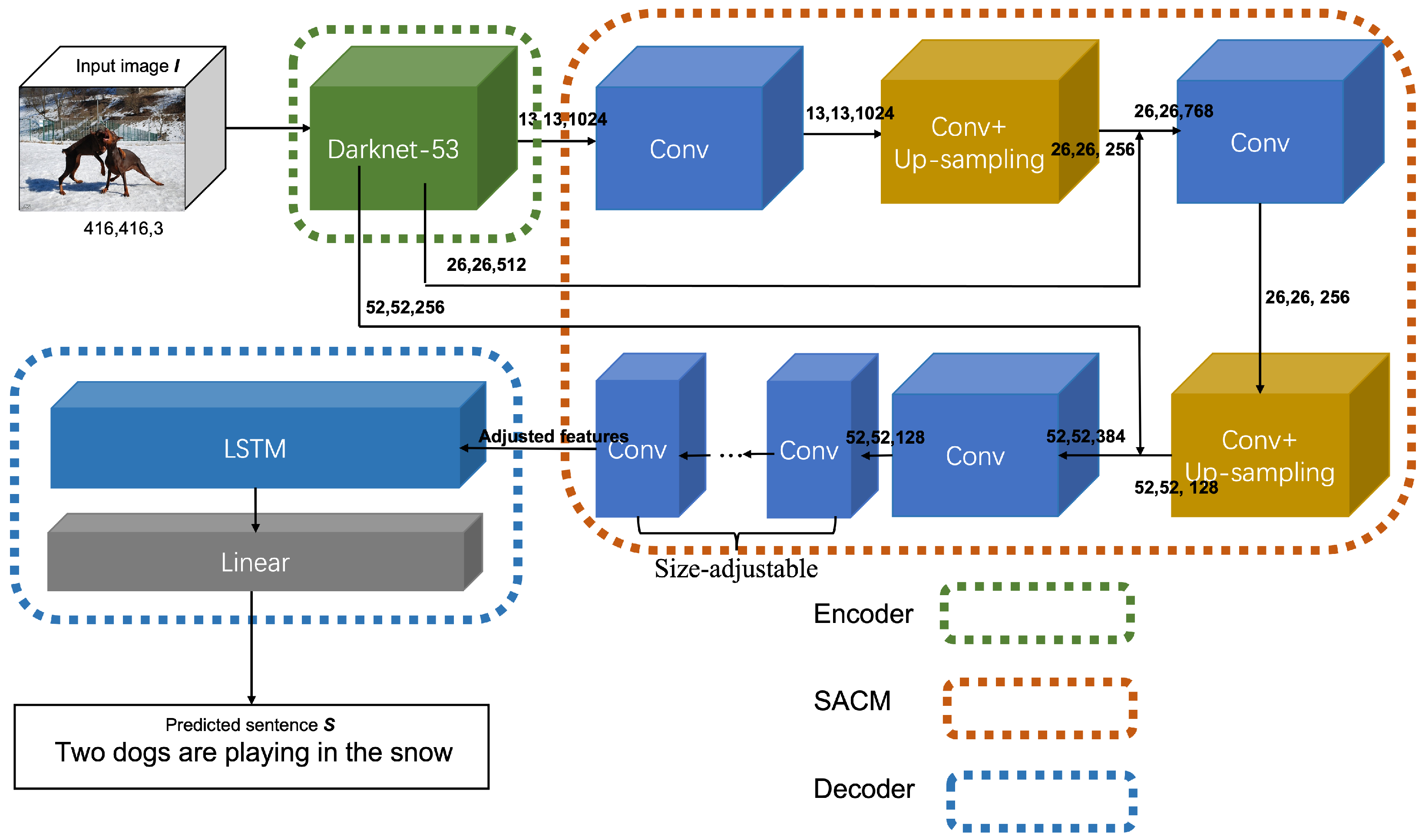
One of the main considerations in this paper is to keep the performance while reducing the computation costs with a smaller-size feature map. For this purpose, we propose to insert a SACM between the encoder and the decoder. SACM is a size-adjustable convolutional module that consists of several convolutional layers for feature extraction and a few additional convolutional layers for dimension reduction. By increasing and decreasing the number of convolutional layers for dimension reduction, we can maintain the balance of performance and cost. The structure of the Darknet-SACM-LSTM model is shown in Figure 2.

Convolutional layers with a $2\times 2$ convolution kernel are applied in SACM for dimension reduction. Incorporating the convolutional layers is a way to form the original feature through $2\times 2$ filters or $1\times 1$ with non-linearity injection. With the $2\times 2$ convolution kernel, each output pixel of the layer is affected by only one pixel in a $2\times 2$ region of the input image after the convolution operation. Firstly, the parameter size will not increase so much with the small-size convolution kernel. For example, when a $2\times 2$ convolutional stack with $C_i$ input channels and $C_o$ output channels is set, the stack is parameterized by $2^2\times C\_i\times C\_o=4C\_i\times C\_o$ weights. A convolutional layer with a $1\times 1$ convolution kernel is equivalent to a cross-channel parametric pooling layer [38]. When the output channel is smaller than the input channel, the convolutional layer can also be used for dimension reduction. Being compared to the pooling layer, the $1\times 1$ convolutional layer is a way to reduce the dimension without affecting the receptive fields of the convolutional layers. For the balance between the final output size and the performance, experiments of SACM with different convolutional layers with $2\times 2$ or $1\times 1$ kernels are set in the simulations. The settings of SACM are shown in

Table 3. Settings of SACM with the original $128\times 52\times 52$ feature size. conv $k_x\times k_y\times c$ is a convolution of kernel size $k_x\times k_y$ with c outputs channels. The last line is the final output $S_f$ size from SACM.

SACM-A	SACM-B	SACM-C	SACM-D	SACM-E
input ($128\times 52\times 52$)
conv2 × 2 × 256	conv2 × 2 × 128	conv2 × 2 × 256	conv2 × 2 × 128	conv2 × 2 × 128
		conv2 × 2 × 256	conv2 × 2 × 128	conv2 × 2 × 128
				conv1 × 1 × 64
$S_f$: 256 × 26 × 26	$S_f$: 128 × 26 × 26	$S_f$: 256 × 13 × 13	$S_f$: 128 × 13 × 13	$S_f$: 64 × 13 × 13

. In addition, the parameters of all the size-adjusting layers do not increase so much. With the settings shown in the table, the module with three layers has the largest number of parameters, 1.05M. In other words, the parameter size of the whole structure decreases to nearly 1/8 of the original size after introducing these extra 1.05M parameters.

After processing by the first five convolutional layers, the size of the feature maps becomes $52\times 52\times 128$. The following adjustable convolutional layers can reduce feature dimension directly for sending to LSTM for caption generation. The SACM performs as a pipeline connecting the encoder and decoder to reduce feature dimensions, saving time and computational costs. After passing through SACM, the dimension-reduced feature maps go through to LSTM for generating captions of the provided images.

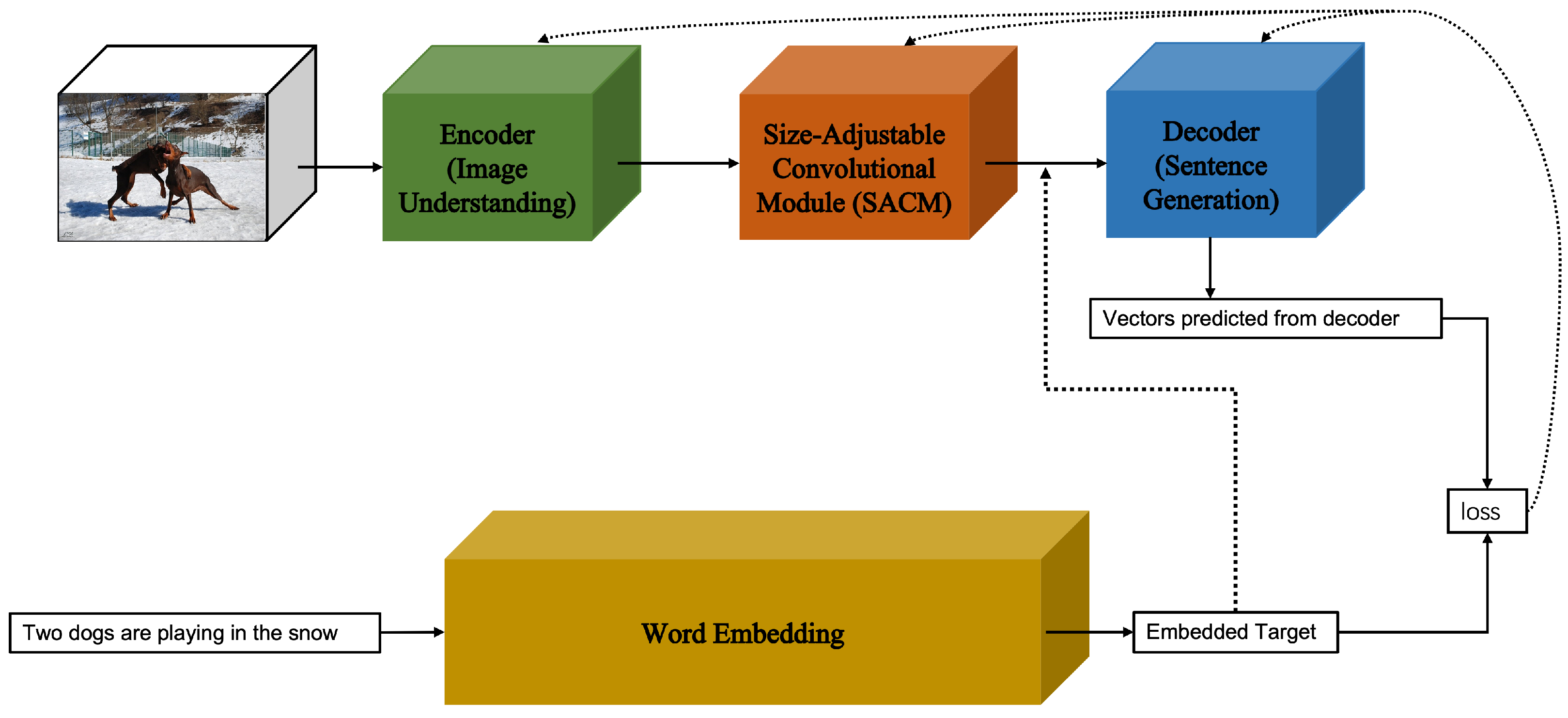
In this paper, experiments were conducted to measure the relationship between the feature size and balance of performance and speed. The final feature size $S_f$ is decreased from 1/2 ($S_f=256\times 26\times 26$) to 1/32 ($S_f=64\times 13\times 13$) of the original feature maps with the $2\times 2$ and $1\times 1$ convolutional layers. Our experiments also trained the SACM with the encoder and the decoder together. With the trainable convolutional encoder of Darknet-53, the training process can be conducted by training the encoder, SACM, and decoder simultaneously with the data, ground truth pairs without fixing the encoder. Therefore, the parameters of Darknet-53, SACM, and LSTM in the proposed model are updated to find the features more useful for learning. The training processing is shown in Figure 3.

Since different people may give different descriptions of the same image, in a general image captioning dataset, each image usually has multiple captions corresponding to it. The dataset like Flickr 8K and MS COCO used in this paper contains five different ground truth captions for each image. Multiple annotations can provide more information and diversity to help the model learn different description styles, have different lexical usages, and learn diffferent semantic expressions. Such a multi-labelling approach helps the model to better adapt to different input images and generate diverse and higher-quality descriptions during testing. During the training process, each caption is set with the image, which it describes as a pair of input and ground truth. In other words, every image is input to the model five times with different captions. For example, the training set of the Flickr 8K dataset contains 6000 images, so there are 30,000 pairs of input and ground truth in the training set.

Word2Index is the word-embedding structure used in this paper to map captions to vectors. At first, the structure collects all the unique words in the dataset to set a vocabulary. As mentioned in Equation (6), the vocabulary scale influences the parameter size. Large-scale vocabulary will increase storage and computational costs. Moreover, it is difficult for the model to obtain enough information from rare words that appear only once or twice and will also affect the model’s prediction of high-frequency words. So, we set thresholds in our experiments at 5 to avoid the effect of rare words on the training effect of the model. Then, the structure maps each word to its unique corresponding index, which is set from 0, to construct the vocabulary for the dataset. The vector of size (sequence_length, index) can map the ground truth into a vector. The value of the corresponding index of the target word is 1, and the others are 0. In addition, the words not in the vocabulary will be instead of <$unk$>.

During the prediction process of image captioning, the model generates a probability distribution at each time step. The word with the highest probability in the distribution is selected as the current output. The prediction continues until either the termination marker is encountered or the maximum generation length is reached. Finally, the generated words are combined to form the final prediction result. Unlike the training process, the model selects only one best sentence as the final generated image caption. To evaluate the model’s performance, the evaluation metrics calculate the similarity between the generated subtitles and each ground truth to derive a composite score, thereby mitigating the effect of subjectivity on the evaluation results.

4. Simulation Results and Comparisons

4.1. Two Datasets

Flickr 8K dataset and MS COCO dataset are used in the experiments. Flickr 8K [8] is a popular dataset with 8000 images collected from Flickr. The training data consist of 6000 images, while the test and evaluation data consist of 1000 images separately. Each image in the dataset has five reference captions annotated by humans. The MS COCO dataset is a very large dataset for image recognition, segmentation, and captioning. There are more than 300,000 images and more than 2 million instances with 80 object categories and five captions per image in the dataset. Many image captioning methods have been tested on these two datasets. In order to draw comparisons of the performance of our model on the MS COCO dataset with other results, the fixed training data used 118,287 images while the evaluation set and testing data set included 5000 images, respectively.

The end-to-end VGG-LSTM model was used as a baseline to compare with the end-to-end Darknet-LSTM model on performance and speed. In the experiment of VGG-LSTM, a pre-trained VGGNet-19 model is used as a feature extractor. To fit the pre-trained model, input images are transformed into $224\times 224\times 3$. As an end-to-end model, the model is fine-tuned for Flickr 8K and MS COCO datasets. The Adam optimizer was used with a base learning rate of ${10}^{-5}$ for both datasets’ models. The dimension of feature maps is set to 4096, while the dimension of hidden layers of LSTM is set to 512 in the VGG-LSTM model. The VGG-LSTM model is trained by minimizing the cross-entropy loss. The Adam optimizer with the same learning rate was applied to the end-to-end Darknet-LSTM model. The input of the original Darknet feature extractor is required to be $416\times 416\times 3$. The batch size is 1 for Flickr 8K and 50 for MS COCO datasets, respectively. The maximum epoch was set to 30. The model with the highest BLEU scores on evaluation data was used for testing.

All of the experiments were run on a computer environment under Ubuntu 20.04, AMD Ryzen 9-3900X CPU with 32GB RAM, and GTX 3090 GPU with 24G memory. Pytorch was used for the deep learning framework. Following the previous research, the rule of captions with at most 20 words was set for both datasets. The specific vocabulary of words was built by particularly removing words that occurred fewer than five times. A vocabulary of 2550 words was created for Flickr 8K, while a vocabulary of 10,321 words was built for MS COCO.

4.2. Setup and Evaluation Metrics

The cross-entropy loss was measured throughout the whole training process. If the dictionary is of size D, the equation of the cross-entropy loss between the predicted word and the target word at time t is as follows:

$$Los{s}_t=-\sum _{j=1}^D{T}_{t,j}log\left(s_{t,j}\right)$$

(7)

and the average loss of the sequence of length N is as follows:

$$Loss=\frac{1}{N}\sum _{t=1}^{N}Los{s}_t$$

(8)

where $T_t$ is the ground truth of the given word at time t. $T_{t,j}$ indicates the probability of the j-th word in the dictionary at the current time step. For example, if the target word at time t is the 7th word in the dictionary, $T_{t,7}$ is 1, and others are 0. $s_{t,j}$ denotes the probability of the model predicting the j-th word at time t. The average loss $Loss$ of the whole predicted sequence length N is calculated with the average function. During the training process, the N is the same as the target sequence, while the N will be fixed in the prediction process. The measured losses in the experiments are the average of all of the cross-entropy losses between the prediction and the target captions.

Some evaluation metrics from machine translation were used in evaluations, including BLEU [39], METEOR [40], ROUGE [41], and CIDEr [42]. BLEU is used to analyze the co-occurrence of n-grams between the predicted captions and ground truth. The n-gram is often used to reflect the precision of the generated captions [39]. It compares a text segment with a set of references to compute a score correlating with a human’s judgement of quality. The semantic propositional image caption evaluation METEOR is calculated based on the weighted harmonic average of single-word recall and precision [40], which can offset the shortcoming of BLEU. It also adds a word-net-based measurement to address issues of synonym matching. ROUGE [41] compares the generated word sequence and word pairs with reference descriptions. There are several different ROUGEs, such as ROUGE-L and ROUGE-N. The most widely used ROUGE-L, in which the longest identical fragment in the generated and ground-truth sentences is defined as the longest common sub-sequence, is selected as one of the evaluation metrics in the experiments. CIDEr [42] is an automatic caption evaluation metric based on consensus. It treats the sentence as a document and uses TF-IDF to calculate the weight of words. The consistency of the generated caption with the reference caption is measured by the cosine distance between the TF-IDF vector representations of two sentences.

4.3. Experimental Results on Flickr 8K

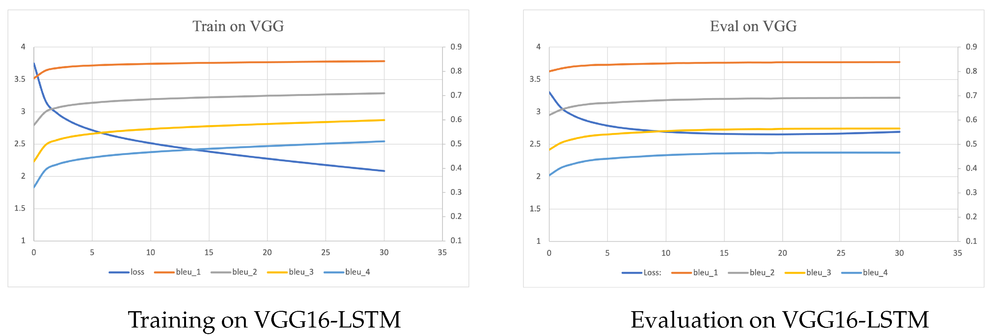
VGGNet is used as an encoder of the baseline model in this paper. After removing the classifier, softmax, and last fully-connected layer, the size of the feature maps is 4096. The changes of both loss values and BLEU scores from 1-gram to 4-gram on both training data (left) and evaluation data (right) are shown in Figure 4. In each figure, the horizontal (x) axis represents the number of learning epochs. The left vertical (y) axis represents the loss values, while the right vertical axis shows the values of BLEU scores. Although the training loss dropped throughout the training process, the evaluation loss slightly increased after 20 learning epochs. As expected, the BLEU scores were lower on the evaluation data than those obtained on the training data.

Because of the limited memory in our computer environment, the experiments on SACM feature selection are set from 1/2 ($S_f=256\times 26\times 26$) of the original size to 1/32 ($S_f=64\times 13\times 13$) of the original size. The training and predicting time cost of SACM with different feature sizes are shown in

Table 4. The cost and performance of SACM with different feature sizes on the testing set for Flickr 8K. B@1 and B@4 denote BLEU-1 and BLEU-4 scores. “No.” denotes the number of learning epochs when the models received the best BLEU-4 score on the evaluation data.

Final Feature Size	Training Time	Predicting Time	B@1	B@4	Loss	No.
${\mathit{S}}_{\mathit{f}}$	(/epoch)	(/1000 Images)
VGG-LSTM (baseline)	15 min	3.75 min	0.798	0.342	2.66	10
128 × 52 × 52	out of memory	out of memory	-	-	-	-
256 × 26 × 26	69 min	18 min	0.822	0.439	2.61	19
128 × 26 × 26	44 min	10.3 min	0.817	0.428	2.65	19
256 × 13 × 13	32 min	5.9 min	0.790	0.419	2.68	17
128 × 13 × 13	28 min	3.9 min	0.823	0.439	2.63	17
64 × 13 × 13	25 min	2.8 min	0.809	0.431	2.64	19

. For performance comparison, BLEU-1 and BLEU-4 scores and the cross-entropy loss by SACM on the testing set are also given in Table 4. The results suggest that SACM with $S_f=128\times 13\times 13$ features received the highest BLEU scores with a similar prediction speed to the baseline model of VGG-LSTM.

The results show that the model with the highest BLEU-1 score of 82.3% used $S_f=128\times 13\times 13$ features. Its BLEU-4 score is 0.439, which is the same as that of the model using $S_f=256\times 26\times 26$ features but higher than those of others. On testing 1000 images, the model with $S_f=128\times 13\times 13$ features used 3.9 min, which ran 15 min faster than the model with $S_f=256\times 26\times 26$ features but 1 min slower than the one using $S_f=64\times 13\times 13$ features. The baseline model could neither match the performance of the implemented models nor run faster than the model using $S_f=64\times 13\times 13$ features.

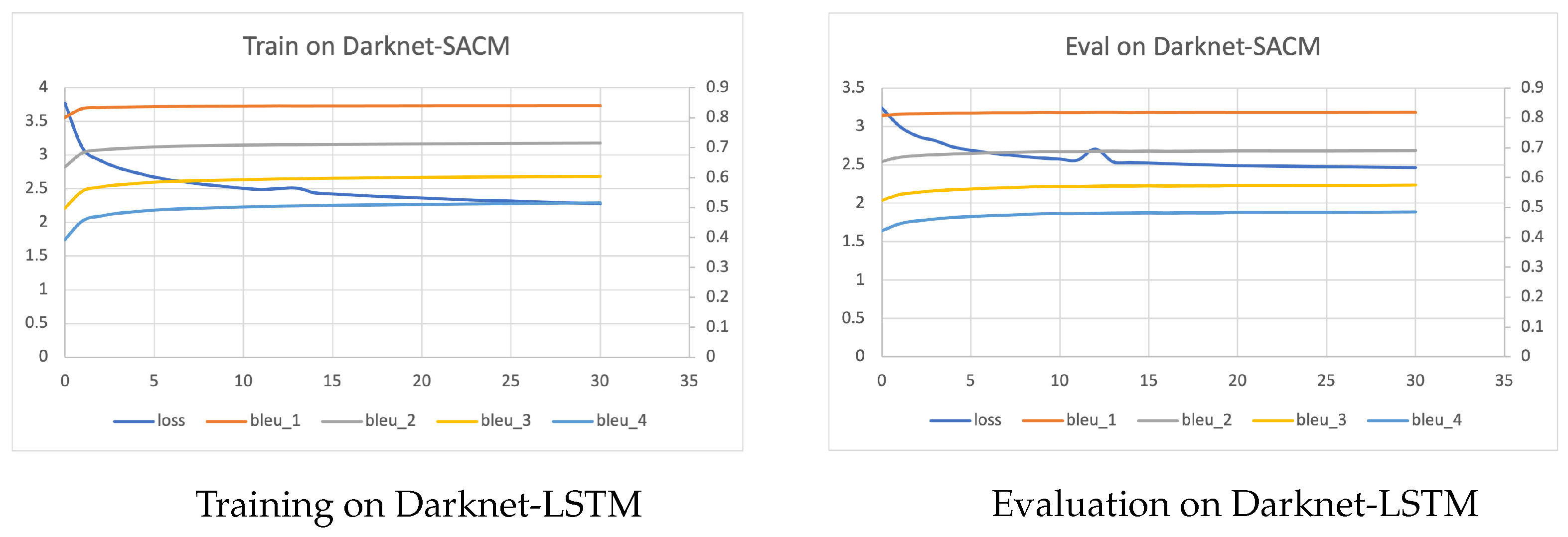
By comparing Figure 4 and Figure 5, it could be seen that SACM with $S_f=64\times 13\times 13$ reached a training loss of 1.7 lower than the training loss of 2.1 by VGG16-LSTM. However, SACM could lead to overfitting on small data sets such as Flickr 8K. It would be important to use the evaluation loss to decide on the final learned model for solving the problems with fewer samples. On Flickr 8K, all the models reached their highest BLEU-4 scores around the 20th training epoch.

4.4. Experimental Results on MS COCO

The results of the baseline encoder VGGNet on the MS COCO dataset were given in Figure 6. It can be seen that both the training loss and the evaluation loss were decreasing from the first epoch until the end. The loss values and BLEU scores changed more in the first 20 epochs. Unlike the results on the Flickr 8K dataset, the best SACMs of different feature sizes on the MS COCO dataset were all received on the 30th epoch. That is, no overfitting appeared on the MS COCO dataset. Because the dictionary size for the MS COCO dataset is nearly 5 times larger than the one for Flickr 8K dataset, only the models using fewer features were tested.

For comparison, the performance of different SACMs on the MS COCO dataset is shown in

Table 5. The cost and performance of SACM with different feature sizes on the testing set for MS COCO. B@1 and B@4 denote BLEU-1 and BLEU-4 scores. “No.” denotes the number of learning epochs when the models received the best BLEU-4 score on the evaluation data.

Final Feature Size	Training Time	Predicting Time	B@1	B@4	Loss	No.
${\mathit{S}}_{\mathit{f}}$	(/epoch)	(/5000 Images)
VGG-LSTM(baseline)	202 min	18.8 min	0.778	0.376	2.51	10
128 × 52 × 52	out of memory	out of memory	-	-	-	-
256 × 26 × 26	out of memory	out of memory	-	-	-	-
128 × 26 × 26	out of memory	out of memory	-	-	-	-
256 × 13 × 13	250 min	31.2 min	0.828	0.434	2.63	30
128 × 13 × 13	240 min	19.5 min	0.831	0.443	2.65	30
64 × 13 × 13	230 min	14.5 min	0.820	0.438	2.63	30

. The B@1, B@4 and No. are the BLEU-1 and BLEU-4 scores and the epoch number of the model that received the best BLEU-4 score on the evaluation data. Similar results were obtained on MS COCO. SACM with features of $S_f=128\times 13\times 13$ outperformed on both BLEU-1 and BLEU-4 scores. Its BLEU-4 score is 0.443, which is higher than those of the others. The baseline model had the lowest BLUE scores. As for the running time, the time rose from 14.5 min to 31.2 min when the final feature size increased from $S_f=64\times 13\times 13$ to $S_f=256\times 13\times 13$ in SACM.

The changes in the loss and BLEU scores on Darknet-SACMs with features of $S_f=128\times 13\times 13$ on both the training and evaluation sets for MS COCO are shown in Figure 7. It is interesting to see that although the learned Darknet-SACMs had higher loss values on both the training and the evaluation set than the learned VGG-LSTM, the learned Darknet-SACMs were able to have higher BLEU scores. This indicates that the lower entropy-loss values might not necessarily lead to better captions.

4.5. Comparison with SOTA

The experiments in this paper proved the effectiveness of our proposed model and succeeded in dimension optimization. The encoder of the best model is set with Darknet as the backbone, and its output feature is 128 × 13 × 13. To showcase our superiority, we provide a comparison with state-of-the-art results on both the Flickr and MS COCO datasets in

Table 6. Comparisons of our proposed Darknet-LSTM with SACM and some SOTA methods on Flickr 8K dataset. B@1, B@4, M, R, C, and P denote BLEU@1, BLEU@4, METEOR, ROUGE-L, CIDEr, and the model sizes.

Method	B@1	B@4	M	R	C	P
Neuraltalk2 [43]	57.9	16.0	-	-	-	31 M
D-CNN [44]	49.5	20.1	42.5	-	-	-
VGG16-LSTM [45]	62.6	28.7	-	-	-	138 M
Hard-attention [12]	66.0	31.4	24.8	50.3	68.9	149 M
Neural Baby Talk [46]	66.4	32.6	26.2	52.5	84.5	37.7 M
m-RNN [47]	66.9	32.8	25.5	51.1	75.8	180 M
SCST [48]	67.5	33.8	25.8	51.6	76.0	-
Vis-to-Lang [18]	72.9	30.7	27.9	-	54.3	157 M
ResNet with Attention [49]	55.6	33.5	-	-	-	-
AoANet [50]	67.4	33.5	26.7	52.7	84.7	115 M
CNN-Bi-GRU [51]	65.6	39.4	-	-	-	-
Darknet-LSTM (ours)	82.3	43.9	27.3	65.1	104.7	97.7 M
CATANIC [52]	78.8	46.7	-	63.8	136.5	300 M

and

Table 7. Comparisons among our proposed Darknet-LSTM with SACM and some SOTA methods on MS COCO dataset. B@1, B@4, M, R, C, and P denote BLEU@1, BLEU@4, METEOR, ROUGE-L, CIDEr, and the model sizes.

Method	B@1	B@4	M	R	C	P
Hard Attention [12]	71.7	25.0	23.04	-	-	149 M
Adaptive Attention [17]	74.2	33.2	26.6	-	108.5	-
Actor–Critic Sequence [53]	77.8	33.7	26.4	55.4	110.2	-
Convolutional Image Captioning [54]	71.1	28.7	24.4	52.2	175	189.3 M
CNN Language Model [55]	72.6	30.3	24.6	-	96.1	-
SCST [48]	78.1	35.2	27.0	56.3	114.7	-
Up-Down [16]	80.2	36.9	27.6	57.1	117.9	108 M
GCN-LSTM [56]	77.4	37.1	28.1	57.2	117.1	-
SGAE [57]	81.0	38.5	28.2	58.6	123.8	-
AoANet (ResNeXt-101 Grid) [50]	81.0	39.4	29.1	58.9	126.9	115 M
X-Transformer [58]	81.9	40.3	29.6	59.5	131.1	11 B
RSTNet [59]	82.1	40.0	29.6	59.5	131.9	54 M/70 M
GET [60]	81.6	39.7	29.4	59.1	130.3	110 M
DLCT [19]	82.4	40.6	29.8	58.8	133.3	-
PureT [61]	82.8	41.4	30.1	60.4	136.0	-
ExpansionNet V2 [62]	83.3	42.1	30.4	60.8	138.5	129.6 M
BLIP-2 ViT-G OPT [63]	-	42.4	-	-	144.5	2700 M
Darknet-LSTM (ours)	83.1	44.3	32.8	65.7	148.0	108.2 M
OFA [64]	-	44.9	32.5	-	154.9	-
mPLUG [65]	-	46.5	32.0	-	155.1	510 M

, respectively. The best scores for each metric are highlighted in bold, and we also include the number of parameters used for prediction to compare prediction speeds.

As we can see from the table, our model shows competitive performance. Specifically, it outperforms the original CNN+RNN-based methods, indicating that our critical designs are effective for image captioning tasks. In addition, our model’s performance is better than many large-scale models. This suggests that further research on the encoder–decoder architecture could inspire new efforts in this area.

Hybrid attention-based CNN-Bi-GRU [52] proposed a hybridized attention-based deep neural network (DNN) model. The model consists of an Inception-v3 convolutional neural network (CNN) encoder to extract image features, a visual attention mechanism to capture significant features, and a bidirectional gated recurrent unit (Bi-GRU) with an attention decoder to generate the image captions. CATANIC [52] applied the AoANet with DenseNet169 as the encoder to extract the initial features of the images and the modified transformer model as the decoder to transform the image feature vector into an image caption.

Our model outperforms most of the previous models on the Flickr 8K dataset across all metrics in both single and ensemble configurations. Our model outperforms other models by BLEU-1 and ROUGE-L. However, the CATANIC model has a slightly higher score in BLEU-4 and CIDER-D despite having a parameter size almost twice as large as ours, with differences of only 0.03 and 0.3, respectively.

More and more large-scale models are appearing and performing better and better. ExpansionNet V2 [62] applied block static expansion, which distributes and processes the input over a heterogeneous and arbitrarily big collection of sequences characterized by a different length compared to the input one. OFA [64] follows the previous research to adopt the encoder–decoder framework as the unified architecture. Especially, both the encoder and the decoder are stacks of transformer layers. A transformer-based encoder layer consists of a self-attention and a feed-forward network (FFN), while a transformer-based decoder layer has a cross-attention network more than the encoder for building the connection between the decoder and the encoder output representations. The mPLUG [65] introduces a new asymmetric vision-language architecture with novel cross-modal skip-connections; it consists of N skip-connected fusion blocks to address two fundamental problems of information asymmetry and computation efficiency in cross-modal alignment. This model adapts the connected attention layer to each S asymmetric co-attention layer.

Our model achieved better results than the previous ExpansionNet V2 on the MSCOCO dataset, with improvements of 1.1 BLEU-4, 2.4 METEOR, 4.9 ROUGE-L, and 10.0 CIDEr-D. Compared to other models, our proposed model outperformed them by 0.3 METEOR and 0.57 ROUGE-L. However, our model was less efficient with the OFA and mPLUG on BLEU-4 and CIDER scores. Despite this, our experiments have shown that the performance of approaches can be improved with larger datasets. Additionally, our best model could speed up predictions with a smaller size than attention-based and transformer-based large-scale models.

To balance the performance and the cost, Ref. [12] introduced an attention-based image captioning model focusing on generating informative captions while considering computational efficiency. The method received a 71.8 BLEU-1 score and a 25.0 BLEU-4 score on the MS COCO dataset. In [17], the authors presented an adaptive attention mechanism that learns to attend to image regions for caption generation selectively, and this method received a 74.8 BLEU-1 score and 33.6 BLEU-4 score. The method proposed in [53] was an actor–critic framework for training image captioning models. It tried to establish a balance via a trade-off between computational cost and captioning performance and received a 33.7 BLEU-4 score. Ref. [55] explored the use of language convolutional neural networks (CNNs) for image captioning, discussed the trade-off between computational cost and captioning performance, and received a 72.6 BLEU-1 score and 30.3 BLEU-4 score. Ref. [54] introduced a convolutional approach to image captioning that focused on reducing the computational cost while maintaining competitive performance. With the help of linear units, this model received a 71.1 BLEU-1 score and a 28.7 BLEU-4 score.

With several convolutional layers, our model performs better than most existing CNN+RNN models and transformer-based models and received comparable results to those of the SOTA models with much smaller model sizes than the SOTA models.

4.6. Qualitative Analysis

Figure 8 shows prediction examples by our models with encoders with different output sizes on the Flickr 8K validation set, which shows reasonable prediction results. The wrong parts of a caption are marked. The GT caption is one of the five targets for evaluating the predicted sentence in the dataset. Compared with the ground truth captions, our best model with the encoded feature of size $S_f=128\times 13\times 13$ has obvious advantages in recognizing objects and some relative details. This advantage maybe comes from the suitable feature with less loss of important information for the decoder.

5. Conclusions

The detection of object classes and positions and their relationships should be considered in solving image captioning tasks. Therefore, the Darknet for object detection is the backbone of our proposed image captioning model. SACM, the size-adjustable convolutional module, is designed for feature extraction and dimension reduction in this paper. With the SACM, convolutional layers are applied for feature dimension reduction while losing less important information on global and local features. With feature dimension reduction, the parameters of the whole model are smaller. With the convolutional layers, the feature size is reduced while expanding the depth of the network for receiving high-level semantic and contextual information. Faster implementation and better performance could be achieved simultaneously in our end-to-end image captioning system with a pre-trained Darknet, SACM, and LSTM.

The end-to-end neural network system proposed in this paper, Darknet-SACM-LSTM, is trained to maximize the likelihood of the correct words in the final sentence describing the given image. After training, our proposed systems can automatically generate a descriptive caption in plain English for a given image. Experiments on the Flickr 8K and MS COCO datasets show the robustness of our Darknet-SACM-LSTM system in terms of speed and several metrics of BLEU scores, METEOR, ROUGE, and CIDEr. By using one or more convolutional layers, SACM could reduce the number of features, speed up the predicting process, and maintain the performance of sentence quality measured by using both the cross-entropy loss and BLEU score.

The experimental results also indicate that neither the best training loss nor the best evaluating loss could let the learned systems with the highest metrics engage in image captioning. By modifying the cross-entropy loss function, it would be necessary to explicitly consider the relationships between items and their positions in the images. The modified loss functions might help the image captioning system to achieve better metrics. Meanwhile, all the parameters in our proposed Darknet-SACM-LSTM are trainable. It would be interesting to know which parts should be adaptive and which parts could be fixed. Even a faster system could be implemented by fixing some parameters besides the feature reductions.

References

1. Staniūtė, R.; Šešok, D. A systematic literature review on image captioning. Appl. Sci. 2019, 9, 2024. [Google Scholar] [CrossRef]
2. Vinyals, O.; Toshev, A.; Bengio, S.; Erhan, D. Show and tell: A neural image caption generator. In Proceedings of the IEEE Conference on Computer Vision and Pattern Recognition, Boston, MA, USA, 7–12 June 2015; pp. 3156–3164. [Google Scholar]
3. Hossain, M.Z.; Sohel, F.; Shiratuddin, M.F.; Laga, H. A comprehensive survey of deep learning for image captioning. ACM Comput. Surv. (CsUR) 2019, 51, 1–36. [Google Scholar] [CrossRef]
4. Farhadi, A.; Hejrati, M.; Sadeghi, M.A.; Young, P.; Rashtchian, C.; Hockenmaier, J.; Forsyth, D. Every picture tells a story: Generating sentences from images. In Proceedings of the Computer Vision–ECCV 2010: 11th European Conference on Computer Vision, Heraklion, Crete, Greece, 5–11 September 2010; Proceedings, Part IV 11. Springer: Berlin/Heidelberg, Germany, 2010; pp. 15–29. [Google Scholar]
5. Li, S.; Kulkarni, G.; Berg, T.; Berg, A.; Choi, Y. Composing simple image descriptions using web-scale n-grams. In Proceedings of the Fifteenth Conference on Computational Natural Language Learning, Portland, OR, USA, 23–24 June 2011; pp. 220–228. [Google Scholar]
6. Kulkarni, G.; Premraj, V.; Ordonez, V.; Dhar, S.; Li, S.; Choi, Y.; Berg, A.C.; Berg, T.L. Babytalk: Understanding and generating simple image descriptions. IEEE Trans. Pattern Anal. Mach. Intell. 2013, 35, 2891–2903. [Google Scholar] [CrossRef]
7. Gong, Y.; Wang, L.; Hodosh, M.; Hockenmaier, J.; Lazebnik, S. Improving image-sentence embeddings using large weakly annotated photo collections. In Proceedings of the Computer Vision–ECCV 2014: 13th European Conference, Zurich, Switzerland, 6–12 September 2014; Proceedings, Part IV 13. Springer: Berlin/Heidelberg, Germany, 2014; pp. 529–545. [Google Scholar]
8. Hodosh, M.; Young, P.; Hockenmaier, J. Framing image description as a ranking task: Data, models and evaluation metrics. J. Artif. Intell. Res. 2013, 47, 853–899. [Google Scholar] [CrossRef]
9. Ordonez, V.; Kulkarni, G.; Berg, T. Im2text: Describing images using 1 million captioned photographs. Adv. Neural Inf. Process. Syst. 2011, 24, 1–9. [Google Scholar]
10. Sun, C.; Gan, C.; Nevatia, R. Automatic concept discovery from parallel text and visual corpora. In Proceedings of the IEEE International Conference on Computer Vision, Santiago, Chile, 7–13 December 2015; pp. 2596–2604. [Google Scholar]
11. Kiros, R.; Salakhutdinov, R.; Zemel, R.S. Unifying visual-semantic embeddings with multimodal neural language models. arXiv 2014, arXiv:1411.2539. [Google Scholar]
12. Xu, K.; Ba, J.; Kiros, R.; Cho, K.; Courville, A.; Salakhudinov, R.; Zemel, R.; Bengio, Y. Show, attend and tell: Neural image caption generation with visual attention. In Proceedings of the International Conference on Machine Learning, PMLR, Lille, France, 6–11 July 2015; pp. 2048–2057. [Google Scholar]
13. Yao, T.; Pan, Y.; Li, Y.; Qiu, Z.; Mei, T. Boosting image captioning with attributes. In Proceedings of the IEEE International Conference on Computer Vision, Venice, Italy, 22–29 October 2017; pp. 4894–4902. [Google Scholar]
14. You, Q.; Jin, H.; Wang, Z.; Fang, C.; Luo, J. Image captioning with semantic attention. In Proceedings of the IEEE Conference on Computer Vision and Pattern Recognition, Las Vegas, NV, USA, 27–30 June 2016; pp. 4651–4659. [Google Scholar]
15. Girshick, R. Fast r-cnn. In Proceedings of the IEEE International Conference on Computer Vision, Santiago, Chile, 7–13 December 2015; pp. 1440–1448. [Google Scholar]
16. Anderson, P.; He, X.; Buehler, C.; Teney, D.; Johnson, M.; Gould, S.; Zhang, L. Bottom-up and top-down attention for image captioning and visual question answering. In Proceedings of the IEEE Conference on Computer Vision and Pattern Recognition, Salt Lake City, UT, USA, 18–23 June 2018; pp. 6077–6086. [Google Scholar]
17. Lu, J.; Xiong, C.; Parikh, D.; Socher, R. Knowing when to look: Adaptive attention via a visual sentinel for image captioning. In Proceedings of the IEEE Conference on Computer Vision and Pattern Recognition, Honolulu, HI, USA, 21–26 July 2017; pp. 375–383. [Google Scholar]
18. Li, X.; Yuan, A.; Lu, X. Vision-to-language tasks based on attributes and attention mechanism. IEEE Trans. Cybern. 2019, 51, 913–926. [Google Scholar] [CrossRef]
19. Luo, Y.; Ji, J.; Sun, X.; Cao, L.; Wu, Y.; Huang, F.; Lin, C.W.; Ji, R. Dual-level collaborative transformer for image captioning. In Proceedings of the AAAI Conference on Artificial Intelligence, Virtual, 2–9 February 2021; Volume 35, pp. 2286–2293. [Google Scholar]
20. Zhou, L.; Palangi, H.; Zhang, L.; Hu, H.; Corso, J.; Gao, J. Unified vision-language pre-training for image captioning and vqa. In Proceedings of the the AAAI Conference on Artificial Intelligence, New York, NY, USA, 7–12 February 2020; Volume 34, pp. 13041–13049. [Google Scholar]
21. Gan, Z.; Li, L.; Li, C.; Wang, L.; Liu, Z.; Gao, J. Vision-language pre-training: Basics, recent advances, and future trends. Found. Trends Comput. Graph. Vis. 2022, 14, 163–352. [Google Scholar] [CrossRef]
22. Wang, W.; Bao, H.; Dong, L.; Bjorck, J.; Peng, Z.; Liu, Q.; Aggarwal, K.; Mohammed, O.K.; Singhal, S.; Som, S.; et al. Image as a Foreign Language: BEiT Pretraining for Vision and Vision-Language Tasks. In Proceedings of the the IEEE/CVF Conference on Computer Vision and Pattern Recognition, Vancouver, BC, Canada, 18–22 June 2023; pp. 19175–19186. [Google Scholar]
23. Vinyals, O.; Toshev, A.; Bengio, S.; Erhan, D. Show and tell: Lessons learned from the 2015 mscoco image captioning challenge. IEEE Trans. Pattern Anal. Mach. Intell. 2016, 39, 652–663. [Google Scholar] [CrossRef]
24. Szegedy, C.; Liu, W.; Jia, Y.; Sermanet, P.; Reed, S.; Anguelov, D.; Erhan, D.; Vanhoucke, V.; Rabinovich, A. Going deeper with convolutions. In Proceedings of the IEEE Conference on Computer Vision and Pattern Recognition, Boston, MA, USA, 7–12 June 2015; pp. 1–9. [Google Scholar]
25. Simonyan, K.; Zisserman, A. Very deep convolutional networks for large-scale image recognition. arXiv 2014, arXiv:1409.1556. [Google Scholar]
26. ResNet, A.; VGGNet, I. Understanding Various Architectures of Convolutional Networks. 2019, p. 24. Available online: https://cv-tricks.com/cnn/understand-resnet-alexnetvgg-inception/ (accessed on 19 July 2023).
27. Krizhevsky, A.; Sutskever, I.; Hinton, G.E. Imagenet classification with deep convolutional neural networks. Adv. Neural Inf. Process. Syst. 2012, 25, 1–9. [Google Scholar] [CrossRef]
28. Zeiler, M.D.; Fergus, R. Visualizing and understanding convolutional networks. In Proceedings of the European Conference on Computer Vision, Zurich, Switzerland, 8–14 September 2014; Springer: Berlin/Heidelberg, Germany, 2014; pp. 818–833. [Google Scholar]
29. Redmon, J.; Divvala, S.; Girshick, R.; Farhadi, A. You only look once: Unified, real-time object detection. In Proceedings of the IEEE Conference on Computer Vision and Pattern Recognition, Las Vegas, NV, USA, 27–30 June 2016; pp. 779–788. [Google Scholar]
30. Jocher, G.; Chaurasia, A.; Qiu, J. YOLO by Ultralytics. Available online: https://github.com/ultralytics/ (accessed on 19 July 2023).
31. Redmon, J.; Farhadi, A. YOLO9000: Better, faster, stronger. In Proceedings of the IEEE Conference on Computer Vision and Pattern Recognition, Honolulu, HI, USA, 21–26 July 2017; pp. 7263–7271. [Google Scholar]
32. Terven, J.; Cordova-Esparza, D. A Comprehensive Review of YOLO: From YOLOv1 to YOLOv8 and Beyond. arXiv 2023, arXiv:2304.00501. [Google Scholar]
33. Hochreiter, S. The vanishing gradient problem during learning recurrent neural nets and problem solutions. Int. J. Uncertain. Fuzziness Knowl.-Based Syst. 1998, 6, 107–116. [Google Scholar] [CrossRef]
34. Jocher, G.; Chaurasia, A.; Qiu, J. Word Embeddings: Encoding Lexical Semantics. Available online: https://pytorch.org/tutorials/beginner/nlp/word_embeddings_tutorial.html#getting-dense-word-embeddings (accessed on 19 July 2023).
35. Forsyth, D. Object detection with discriminatively trained part-based models. Computer 2014, 47, 6–7. [Google Scholar] [CrossRef]
36. Girshick, R.; Donahue, J.; Darrell, T.; Malik, J. Rich feature hierarchies for accurate object detection and semantic segmentation. In Proceedings of the IEEE Conference on Computer Vision and Pattern Recognition, Columbus, OH, USA, 23–28 June 2014; pp. 580–587. [Google Scholar]
37. Redmon, J.; Farhadi, A. Yolov3: An incremental improvement. arXiv 2018, arXiv:1804.02767. [Google Scholar]
38. Lin, M.; Chen, Q.; Yan, S. Network in network. arXiv 2013, arXiv:1312.4400. [Google Scholar]
39. Papineni, K.; Roukos, S.; Ward, T.; Zhu, W.J. Bleu: A method for automatic evaluation of machine translation. In Proceedings of the 40th annual meeting of the Association for Computational Linguistics, Philadelphia, PA, USA, 7–12 July 2002; pp. 311–318. [Google Scholar]
40. Banerjee, S.; Lavie, A. METEOR: An automatic metric for MT evaluation with improved correlation with human judgments. In Proceedings of the ACL Workshop on Intrinsic and Extrinsic Evaluation Measures for Machine Translation and/or Summarization, Ann Arbor, MI, USA, 29 June 2005; pp. 65–72. [Google Scholar]
41. Doddington, G. Automatic evaluation of machine translation quality using n-gram co-occurrence statistics. In Proceedings of the Second International Conference on Human Language Technology Research, San Diego, CA, USA, 24–27 March 2002; pp. 138–145. [Google Scholar]
42. Vedantam, R.; Lawrence Zitnick, C.; Parikh, D. Cider: Consensus-based image description evaluation. In Proceedings of the IEEE Conference on Computer Vision and Pattern Recognition, Boston, MA, USA, 7–12 June 2015; pp. 4566–4575. [Google Scholar]
43. Karpathy, A.; Fei-Fei, L. Deep visual-semantic alignments for generating image descriptions. In Proceedings of the IEEE Conference on Computer Vision and Pattern Recognition, Boston, MA, USA, 7–12 June 2015; pp. 3128–3137. [Google Scholar]
44. Bhalekar, M.; Bedekar, M. D-CNN: A New model for Generating Image Captions with Text Extraction Using Deep Learning for Visually Challenged Individuals. Eng. Technol. Appl. Sci. Res. 2022, 12, 8366–8373. [Google Scholar] [CrossRef]
45. Srivastava, S.; Sharma, H.; Dixit, P. Image Captioning based on Deep Convolutional Neural Networks and LSTM. In Proceedings of the 2022 2nd International Conference on Power Electronics & IoT Applications in Renewable Energy and its Control (PARC), Mathura, India, 21–22 January 2022; IEEE: Piscataway, NJ, USA, 2022; pp. 1–4. [Google Scholar]
46. Lu, J.; Yang, J.; Batra, D.; Parikh, D. Neural baby talk: Generating image descriptions from visual data. In Proceedings of the IEEE Conference on Computer Vision and Pattern Recognition, Salt Lake City, UT, USA, 18–23 June 2018; pp. 7219–7228. [Google Scholar]
47. Mao, J.; Xu, W.; Yang, Y. Generating sequences with recurrent neural networks. In Proceedings of the 28th International Conference on Neural Information Processing Systems-Volume 2, Montreal, QC, Canada, 7–12 December 2015; pp. 1283–1291. [Google Scholar]
48. Rennie, S.J.; Marcheret, E.; Mroueh, Y.; Ross, J. Self-critical sequence training for image captioning. In Proceedings of the IEEE Conference on Computer Vision and Pattern Recognition, Honolulu, HI, USA, 21–26 July 2017; pp. 7008–7024. [Google Scholar]
49. Sethi, A.; Jain, A.; Dhiman, C. Image Caption Generator in Hindi Using Attention. In Advanced Production and Industrial Engineering; IOS Press: Amsterdam, The Netherland, 2022; pp. 101–107. [Google Scholar]
50. Huang, L.; Wang, W.; Chen, J.; Wei, X. Attention on Attention for Image Captioning. In Proceedings of the IEEE Conference on Computer Vision and Pattern Recognition, Long Beach, CA, USA, 15–20 June 2019; pp. 12142–12151. [Google Scholar]
51. Solomon, R.; Abebe, M. Amharic Language Image Captions Generation Using Hybridized Attention-Based Deep Neural Networks. Appl. Comput. Intell. Soft Comput. 2023, 2023, 9397325. [Google Scholar] [CrossRef]
52. Zhang, T.; Zhang, T.; Zhuo, Y.; Ma, F. CATANIC: Automatic generation model of image captions based on multiple attention mechanism. Res. Sq. 2023, preprint. [Google Scholar]
53. Zhang, L.; Sung, F.; Liu, F.; Xiang, T.; Gong, S.; Yang, Y.; Hospedales, T.M. Actor-critic sequence training for image captioning. arXiv 2017, arXiv:1706.09601. [Google Scholar]
54. Aneja, J.; Deshpande, A.; Schwing, A.G. Convolutional image captioning. In Proceedings of the IEEE Conference on Computer Vision and Pattern Recognition, Salt Lake City, UT, USA, 18–23 June 2018; pp. 5561–5570. [Google Scholar]
55. Gu, J.; Wang, G.; Cai, J.; Chen, T. An empirical study of language cnn for image captioning. In Proceedings of the IEEE International Conference on Computer Vision, Venice, Italy, 22–29 October 2017; pp. 1222–1231. [Google Scholar]
56. Yao, T.; Pan, Y.; Li, Y.; Mei, T. Exploring visual relationship for image captioning. In Proceedings of the European Conference on Computer Vision (ECCV), Munich, Germany, 8–14 September 2018; pp. 684–699. [Google Scholar]
57. Yang, X.; Tang, K.; Zhang, H.; Cai, J. Auto-encoding scene graphs for image captioning. In Proceedings of the IEEE/CVF Conference on Computer Vision and Pattern Recognition, Long Beach, CA, USA, 15–20 June 2019; pp. 10685–10694. [Google Scholar]
58. Pan, Y.; Yao, T.; Li, Y.; Mei, T. X-linear attention networks for image captioning. In Proceedings of the IEEE/CVF Conference on Computer Vision and Pattern Recognition, Seattle, WA, USA, 13–19 June 2020; pp. 10971–10980. [Google Scholar]
59. Zhang, X.; Sun, X.; Luo, Y.; Ji, J.; Zhou, Y.; Wu, Y.; Huang, F.; Ji, R. Rstnet: Captioning with adaptive attention on visual and non-visual words. In Proceedings of the IEEE/CVF Conference on Computer Vision and Pattern Recognition, Nashville, TN, USA, 20–25 June 2021; pp. 15465–15474. [Google Scholar]
60. Ji, J.; Luo, Y.; Sun, X.; Chen, F.; Luo, G.; Wu, Y.; Gao, Y.; Ji, R. Improving image captioning by leveraging intra-and inter-layer global representation in transformer network. In Proceedings of the AAAI conference on Artificial Intelligence, Virtual, 2–9 February 2021; Volume 35, pp. 1655–1663. [Google Scholar]
61. Wang, Y.; Xu, J.; Sun, Y. End-to-end transformer based model for image captioning. In Proceedings of the the AAAI Conference on Artificial Intelligence, Washington DC, USA, 7–14 February 2022; Volume 36, pp. 2585–2594. [Google Scholar]
62. Hu, J.C.; Cavicchioli, R.; Capotondi, A. ExpansionNet v2: Block Static Expansion in fast end to end training for Image Captioning. arXiv 2022, arXiv:2208.06551. [Google Scholar]
63. Li, J.; Li, D.; Savarese, S.; Hoi, S. Blip-2: Bootstrapping language-image pre-training with frozen image encoders and large language models. arXiv 2023, arXiv:2301.12597. [Google Scholar]
64. Wang, P.; Yang, A.; Men, R.; Lin, J.; Bai, S.; Li, Z.; Ma, J.; Zhou, C.; Zhou, J.; Yang, H. Ofa: Unifying architectures, tasks, and modalities through a simple sequence-to-sequence learning framework. In Proceedings of the International Conference on Machine Learning, PMLR, Baltimore, MD, USA, 17–23 July 2022; pp. 23318–23340. [Google Scholar]
65. Li, C.; Xu, H.; Tian, J.; Wang, W.; Yan, M.; Bi, B.; Ye, J.; Chen, H.; Xu, G.; Cao, Z.; et al. mPLUG: Effective and Efficient Vision-Language Learning by Cross-modal Skip-connections. arXiv 2022, arXiv:2205.12005. [Google Scholar]
Disclaimer/Publisher’s Note: The statements, opinions and data contained in all publications are solely those of the individual author(s) and contributor(s) and not of MDPI and/or the editor(s). MDPI and/or the editor(s) disclaim responsibility for any injury to people or property resulting from any ideas, methods, instructions or products referred to in the content.
Article Metrics
Citations
Article Access Statistics
Multiple requests from the same IP address are counted as one view.