An Algorithm for Sorting Staggered PRI Signals Based on the Congruence Transform

Abstract

To address the problems of poor adaptability to pulse loss, susceptibility to interfered pulses, and the need of sub-PRI (Pulse Repetition Interval) ranking in the existing signal sorting algorithms, this paper proposes an algorithm for sorting staggered PRI signals based on the congruence transform. According to the analysis of the congruence characteristics of the staggered PRI signal, the proposed algorithm transforms the arrival time of the pulse to a fixed value, based on which the staggered PRI signal sorting and the sub-PRI sequence extraction can be achieved. Simulation results show that the proposed algorithm can effectively sort the staggered PRI signals and obtain the sub-PRI sequence directly without sub-PRI ranking, and, compared to some typical algorithms, it is less affected by the interfered pulses and the pulse loss.

1. Introduction

Sorting radar emitting signal is a continuous and difficult research point in the field of electronic warfare, which aims to separate different radar signals and lays the foundation for radar radiation source feature extraction and identification. Signal sorting usually contains pre-sorting based on radar waveform parameters and PRI (pulse repetition interval) sorting based on pulse sequence time of arrive (TOA) de-interleaving and PRI modulation pattern recognition [1,2,3,4,5]. With the continuous emergence of new radar system, the reconnaissance signal presents the characteristics of complex waveform parameter modulation and serious overlapping of waveform parameters among multiple emitters. The performance of pre-sorting algorithm based on waveform parameters decreases seriously [6], and it is difficult to achieve effective sorting of radar radiation source signals. However, although the pulse sequences are interleaved under the condition of interleaved multiple radar emitters, the correlation between the pulse signals of the same radiation source is not broken. Therefore, the pulse sequence de-interleaving is an effective way to solve the current problem.

There are many classical algorithms for pulse sequence de-interleaving, while these methods are unsustainable in the complex electromagnetic environment, where pulse trains with staggered PRI, pulse losses, and interfered pulses may be existed [7]. For example, statistical histogram algorithms, represented by the cumulative difference histogram (CDIF) algorithm [8] and the CDIF-based sequential difference histogram (SDIF) algorithm [9], are simple to implement, have high sorting efficiencies, and have been applied in practice frequently, while they cannot suppress harmonics because of the pulse loss. The time-delayed autocorrelation histogram algorithms, represented by PRI transform, have a good harmonic suppression capability, while they cannot sort pulse trains with staggered PRI modulation [10,11,12,13]. In response to the problems of classical PRI transform algorithms, Refs. [14,15] addresses the problem of frame period measurement of pulse trains with staggered PRI by combining PRI transform and sequence extraction to reduce the complexity of the environment, which can make PRI judgments on the environment after extracting pulse trains. However, these algorithms have a poor adaptability to pulse loss and interference. In [16], based on the extended correlation method and the eigenvector method, a method is proposed to establish a pulse interval distribution matrix according to the connection between pulse pair intervals and individual pulses, achieving simultaneous harmonic suppression and frame period extraction. The computational complexity of this method remains the same as the PRI transform algorithm, while it requires the ranking of the staggered PRI signal sub-sequence. Refs. [17,18] proposes a frequent term expansion algorithm that can effectively identify staggered PRI signals, and based on the frequent term expansion algorithm, the measure of interest of association patterns is introduced to achieve the sorting and identification of staggered PRI signals in the interleaved pulse sequences, while the algorithm end condition is too complicated for practical implementation. Based on the Ramanujan subspace, Refs. [19,20] proposed a correlation matching method(CMM), which can be used for de-interleaving of staggered sequences, but the performance of anti-loss pulse and interference pulse is not as good as in [16,17,18].

Considering the above-mentioned problems of existing algorithms, this paper proposes a staggered PRI sorting algorithm based on the congruence transform. Based on the congruence between time of arrival and frame period, the proposed algorithm transforms the arrival time of the same radar signal to the same congruence, and thus achieves the sorting identification of staggered PRI signals and the direct extraction of sub-sequences. Simulation results show that the proposed algorithm is less affected by the interfered pulse and pulse loss.

2. Model and Analysis

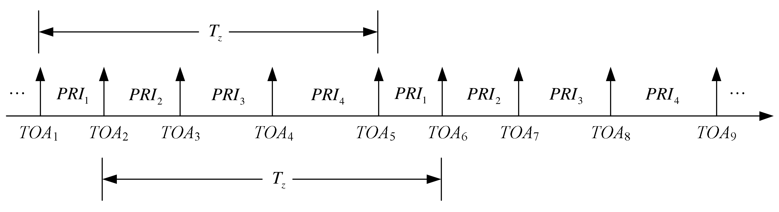
2.1. Signal Model of Pulse Trains with Staggered PRI

When only TOA is considered, the pulse trains detected by the reconnaissance receiver can be written as

$$PT(t)={\displaystyle \sum _{n=1}^N\delta (t-t_n)}$$

(1)

where δ(t) is the impulse excitation function, t_n is the TOA of the nth pulse, and N is the number of pulses.

If t_n = t₁ + (n − 1)T, the pulse sequence has a fixed PRI T. For the staggered PRI signals, t_n = t_k + (n_k − 1)T_z with n_k = 1, 2, …, N_k, which can be regarded as the superposition of multiple fixed PRI pulse sequences. As shown in Figure 1, containing a sub-PRI sequences, T_z is defined as the frame period of the staggered PRI signals, expressed as

$$T_z={\displaystyle \sum _{k=1}^{K}PR{I}_k}$$

(2)

Then, the signal model of pulse trains with staggered PRI modulation is given by

$$\{\begin{array}{l}PT(t)={\displaystyle \sum _{k=1}^K{\displaystyle \sum _{n_k=1}^{N_k}\delta (t-t_k-n_k{T}_z)}}\\ t_k=PR{I}_1+PR{I}_2+\cdots +PR{I}_k\end{array}$$

(3)

The reference PRI signal is the superposition of a time sequence of K fixed PRI signals with the start time of t_k with k = 1, 2, … and K and the repetition period of T_z. The arrival time of the kth fixed PRI signal can be expressed as

$$\{\begin{array}{l}TO{A}_{n_k}^k=t_k+n_k{T}_z\\ t_k=PR{I}_1+PR{I}_2+\cdots +PR{I}_k\end{array}$$

(4)

2.2. Congruence Transform of Staggered PRI Signal

Calculate the remainder of the arrival time of the staggered PRI signal modulo positive integer T_m, we can obtain

$$\mathrm{mod}\left[TO{A}_{n_k}^k,T_m\right]=\mathrm{mod}\left[t_k,T_m\right]+\mathrm{mod}\left[n_k{T}_z,T_m\right]$$

(5)

where mod[·] denotes the remainder operation.

When T_m = T_z, (5) can be rewritten as

$$\mathrm{mod}\left[TO{A}_{n_k}^k,T_m\right]=\mathrm{mod}\left[t_k,T_m\right]$$

(6)

At this point, the arrival time of the staggered PRI signal can be converted to K fixed values, and this process is called the congruent transform in this paper. Since the sub-PRI of the covariant PRI signal is smaller than the frame period T_z, the sub-PRI sequence of the staggered PRI signal can be obtained by combining (4) and (6), as

$$PR{I}_k=\mathrm{mod}\left[t_{k+1},T_m\right]-\mathrm{mod}\left[t_k,T_m\right]$$

(7)

Based on (5)–(7), it is clear that the congruent transform not only transforms the staggered PRI signal arrival time into a finite number of fixed values, but also calculates the sub-PRI sequence from the transformed values.

For example, the congruence transform is conducted on a 3-staggered PRI signal with the PRIs as {57 μs, 78 μs, 65 μs}, obtaining the results shown in Figure 2.

It can be seen that the staggered signals after congruence transform are gathered at three points 29 μs, 86 μs, 164 μs with the frame period of 200 μs. {29 μs, 86 μs, 164 μs} are exactly the t_k of the pulse sequence. Thus, we can obtain the PRIs as {57 μs, 78 μs} by adjacent subtraction operation with {29 μs, 86 μs, 164 μs}. Then, another PRI 65 μs can be obtained by subtraction operation with {57 μs, 78 μs} and 200 μs. {57 μs, 78 μs, 65 μs} are the sub-PRIs of the staggered PRI signal. It can be concluded that the staggered PRI signal sequence undergoes a congruent transform modulo the frame period gathered in (T_z, t_k) with k = 1, 2, and 3.

When T_m ≠ T_z, the first term on the right side of (5) is related to t_k and the second term is related to the pulse number n_k. In such a case, the result of the calculation of (5) is a variable. Therefore, the staggered PRI signal can be sorted based on the congruence transform to obtain the sub-PRI sequence.

Particularly, under the condition that T_m ≠ T_z, we have T_m = mT_z, where m is an integer greater than 1 and smaller than n. Then, (5) can be changed to the following form.

$$\{\begin{array}{l}TO{A}_{n_k}^k=t_k+\Delta t_m+n_m{T}_m\\ n_m=\lfloor \frac{n_k}{m}\rfloor \\ \Delta t_m=\left(\frac{n_k}{m}-n_m\right)T_m\end{array}$$

(8)

where $\lfloor \cdot \rfloor$ denotes rounding down.

Equation (8) can be written as a system of congruent equations modulo T₂, T₃, …, T_m as

$$\{\begin{array}{l}TO{A}_{n_k}^k=m_2{T}_2+\Delta T_2\\ TO{A}_{n_k}^k=m_3{T}_3+\Delta T_3\\ \begin{array}{cc}& ⋮\end{array}\\ TO{A}_{n_k}^k=m_m{T}_m+\Delta T_m\end{array}$$

(9)

where ΔT_m = Δt_m + t_k is the remainder of a certain arrival time modulo T_m. For the remainders ΔT₀, ΔT₁, …, ΔT_M, the combination of (8) and (9) yields

$$\{\begin{array}{l}\Delta T_m=t_k+q{T}_z\\ q=n-m{n}_m\end{array}$$

(10)

where q is a non-negative integer.

It can be seen from (10) that the remainders ΔT₀, ΔT₁, …, ΔT_M have a same remainder t_k with the modulo of T_z, i.e., the arrival time of the k-th PRI fixed pulse sequence at T_m = mT_z can also be changed to a fixed value by the operation of (8)–(10), and the sub-PRI can be calculated by (7).

For example, the congruence transform is conducted on the same data of Figure 2 with T_m = mT_z (m = 2) as a mode, giving the results shown in Figure 3. It can be seen that the staggered PRI signals after congruent transform are gathered at six points 29 μs, 86 μs, 164 μs, 229 μs, 286 μs, 364 μs, where 400 μs is two times the frame period of the staggered PRI signal. {29 μs, 86 μs, 164 μs,229 μs, 286 μs, 364 μs} are exactly the t_k of the pulse sequence. Thus, we can obtain the PRIs as {57 μs, 78 μs, 65 μs, 57 μs, 78 μs} by adjacent subtraction operation with set {29 μs, 86 μs, 164 μs,229 μs, 286 μs, 364 μs}. Then, another PRI 65 μs can be obtained by subtraction operation with {57 μs, 78 μs, 65 μs, 57 μs, 78 μs} and 400 μs. {57 μs, 78 μs, 65 μs, 57 μs, 78 μs, 65 μs} are the sub-PRIs of the staggered PRI signal.Therefore, it can be concluded that, when the staggered PRI signal is congruently transformed with mT_z as a mode, the signal sequence can be gathered at (T_z, t_k) with k = 1, 2, 3, 4, 5, and 6.

Since (T_z, t_k) of different radar signal sequences are unique, it is possible to distinguish different radar radiation sources by the congruence transform, thus realizing PRI de-interleaving. Moreover, all arrival times of the signal sequences are converted into constants during the congruence transform, which does not involve the calculation of arrival times between adjacent pulses, so that the effect of pulse loss can be avoided.

3. Sorting Algorithm Based on Congruent Transform

3.1. Principle of Signal Sorting Algorithm

Although it is unique, for an unsorted radar signal sequence, the value of (T_z, t_k) is unknown. For sorting the staggered signal, T_z and t_k need to be estimated. Therefore, this paper proposes a joint estimation algorithm of T_z and t_k.

It can be obtained via the analysis in Section 2 that the residual of the signal after the congruent transform is t_k, then we have

$$H\left(TOA,T_m,t_k\right)-t_k=0$$

(11)

where H(•) denotes the congruent transform of the signal sequence, and T_z is the mode of the congruent transform. Obviously, (11) only holds if T_m = T_z or T_m = mT_z. From (10), it is clear that the result of congruence transform is not only related to t_k, but also related to the positive integer q. The difference between the result of congruence transform and t_k is a variable.

In such a case, the estimation of T_z and t_k can be achieved by a function of (T_z, t_k), given by

$$f(T_z,t_k)={\displaystyle \sum _{n=1}^N{\Vert 1-\left|sign\left[\mathrm{H}\left(TOA(k,n),T_m,t_k\right)-t_k\right]\right|\Vert }_0}$$

(12)

where sign(•) denotes the sign function and ‖•‖₀ denotes the L₀ norm. The function f(T_z, t_k) is calculated for the interleaved pulse sequence shown in Figure 4b, and the graph of result is obtained as shown in Figure 4c.

Comparing Figure 4a with Figure 4c, it can be seen that the number of pulse statistics with zero calculated results in (11) is shown as a peak in the plot, and the peak of f(•) of the same signal sequence has a line distribution, which is consistent with the real PRI distribution shown in Figure 4a. However, the interleaved pulse sequences will make the calculation results have anomalous peak points as shown in Figure 4c, which need to be identified and removed in the parameter estimation process.

Comparing Figure 4a–c, it can be seen that this plot can distinguish the interleaved pulse sequences, and the distribution of peak positions from f(•) can not only obtain the pulse sequences, but also achieve the joint estimation of T_z and t_k via a point-by-point search of the two-dimensional parameters, i.e.,

$$({\widehat{T}}_z,{\widehat{t}}_k)=\arg \underset{T_z,t_k}{\max }\left({\displaystyle \sum _{n=1}^N{\Vert 1-\left|sign\left[H\left(TOA(k,n),T_z,t_k\right)-t_k\right]\right|\Vert }_0}\right)$$

(13)

However, the range of values of (T_z, t_k) is too large, and thus the point-by-point search method will confront the contradiction of step size and computational load, which is not conducive to practical applications. To solve this problem, this paper proposes a method which further constrains the definition domain of the pulse sequence according to the relationship between arrival time and (T_z, t_k), and performs a targeted search for the parameters.

Firstly, as t_k is the first pulse arrival time of the pulse sequence, t_k ∈ Φ with Φ = {TOA₁, TOA₂, TOA₃, …, TOA_Q}, Q indicates the number of pulses to be processed, so the search for t_k is done in the order of the pulse sequence arrival time, avoiding the step size selection problem.

Secondly, T_z is the difference between the arrival times of certain two pulses, i.e.,

$$T_z=TO{A}_i-TO{A}_k=TO{A}_i-t_k,\begin{array}{cc}& i>k\end{array}$$

(14)

In the case of pulse loss, T_z = (TOA_i – t_k)/p, i > k, p = 1, 2, …, P, where P − 1 is the number of dropped pulses, the domain of T_z is thus Ψ = {T_z|T_z = (TOA_i – t_k)/p, i > k, p = 1, 2, …, P}.

Then, (13) can be written as

$$({\widehat{T}}_z,{\widehat{t}}_k)=\arg \underset{\begin{array}{l}{T}_z\in \Psi ,\\ t_k\in \Phi \end{array}}{\max }\left({\displaystyle \sum _{n=1}^N{\Vert 1-\left|sign\left[\mathrm{H}\left(TOA(k,n),T_z,t_k\right)-t_k\right]\right|\Vert }_0}\right)$$

(15)

The estimation of the frame period T_z and the arrival time t_k of the first pulse can be achieved by solving (15).

In addition, due to the interaction between interleaved pulses and the existence of interference pulses, in the process of congruent transform on the signal sequence, certain interference pulses will have the same transform residuals as the real pulse sequence. It makes the anomalous peak points present in the graph shown in Figure 4c. Comparing the peak distribution of the real pulse sequence with the distribution of the anomalous peak points in the figure, we can see that the anomalous peak points exist in isolation, while the peaks of the real pulse sequence are in a linear distribution. Therefore, the influence of the interference pulse can be eliminated according to the different distribution characteristics of the peak points.

3.2. Flow of Signal Sorting Algorithm

According to the above analysis, the specific steps of the proposed signal sorting algorithm are summarized as follows:

Step 1: initialize the range of values of T_z ∈ [T_min, T_max], the maximum number of allowed dropped pulses P, and the counter count = 0, and input the pulse sequence to be sorted;

Step 2: select the first Q arrival times of the pulse sequence as the set Φ, and construct the set Ψ according to the number of dropped pulses P and the range of [T_min, T_max];

Step 3: select the qth arrival time TOA_q such that t_k = TOA_q and combine it with the elements of the set Ψ to compute f(T_z, t_k) and take its maximum value y_q;

Step 4: the graph of f(T_z, t_k) is obtained by rearranging the size according to (T_z, t_k);

Step 5: detect straight line detection on the graph, if the straight line exists, the frame period and arrival time corresponding to its starting position is the estimated value of (T_z, t_k); if the straight line does not exist, set count = count + 1; if count is less than the maximal value, go to step 3, if count is greater than or equal to the maximal value, stop the algorithm;

Step 6: extracting the signal sequence according to the peak position of the graph, estimating (T_z, t_k), performing the congruent transform on the extracted pulse sequence and determining the type of PRI variation.

3.3. Computational Complexity Analysis

According to its steps, the proposed algorithm needs to calculate the function f(T_z, t_k) for each pulse in its operation, resulting in a computational complexity of O(N²). Besides, the complexities of the straight-line detection and the pulse extraction are both O(N). Hence, the overall computational cost of the proposed algorithm is O[(N + 2) N], which is comparable to that of the PRI transform algorithm.

4. Simulation and Analysis

To verify the effectiveness and stability of the proposed algorithm in complex electromagnetic environment, two simulation experiments are conducted with the following scenarios and parameter settings.

4.1. Experiment 1: Assess the Algorithm Effectiveness under Different Signal Environments

Simulation parameters: 4 radar emitters, with the radiation source parameters as (1) 278 μs fixed PRI signal sequence, first pulse arrival time 0 μs; (2) 261 μs PRI fixed signal sequence, first pulse arrival time 37 μs; (3) 3-parameter PRI signal sequence of {90 μs, 115 μs, 142 μs}, first pulse arrival time is 25 μs; (4) 5-parameter PRI signal sequence of {61 μs, 65 μs, 71 μs, 73 μs, 69 μs}, first pulse arrival time 11 μs.

Figure 5 gives the results of the proposed algorithm in the scene 5 signal environment shown in

Table 1. Comparison of the sorting results of different algorithms.

No.	Scene	Algorithm in [10]	Algorithm in [16]	Algorithm in [18]	Proposed Algorithm
1	Radar 1, 2	[1,2]	[1,2]	[1,2]	[1,2]
2	Radar 3, 4	—	[3,4], N-sub	[3,4], N-sub	[3,4], Y-sub
3	Radar 1, 2, 3	[1,2]	[1,2,3], N-sub	[1,2,3], N-sub	[1,2,3], Y-sub
4	Radar 1, 3, 4	[1]	[1,3,4], N-sub	[1,3,4], N-sub	[1,3,4], Y-sub
5	Radar 1, 2, 3, 4	[1,2]	[1,2,3,4], N-sub	[1,2,3,4], N-sub	[1,2,3,4], Y-sub

Note: “—” indicates that the algorithm does not have this function, the numbers inside [•] indicate the serial numbers of the radar emitters, Y-sub indicates the algorithm can obtain the sub-sequence directly, while N-sub indicates the algorithm cannot do it.

. From Figure 5b, it can be seen that the proposed algorithm can separate the radar signals of 4 overlapping parts after the f(•) function calculation, and effectively estimate the frame period value and the PRI value of fixed re-frequency of the covariance signal, as well as the first pulse arrival time of the pulse sequence. From Figure 5c, it can be seen that the proposed algorithm can effectively extract the radar radiation signals and can extract the sub-sequence of the staggered PRI signals.

For the overlapping signal sequences in different signal environments shown in Table 1, the algorithm of [10,16,18] and this paper are used to process them, and the processing results are shown in Table 1. From Table 1, it can be seen that the proposed algorithm can correctly sort the staggered PRI signals as well as directly extract the sub-PRI sequences. The algorithm of [16,18] can correctly sort the PRI signals but cannot directly obtain the sub-PRI sequences and the algorithm based on PRI transform in [10] cannot sort the PRI signals.

4.2. Experiment 2: The Effect of Pulse Loss and Interference Pulse on the Proposed Algorithm

To verify the performance of the proposed algorithm in complex electromagnetic environments, scene 5 shown in Table 1 is used to from two aspects: pulse loss and interference pulse. The scene 5 parameters of the TOA model are shown in

Table 2. The scene 5 parameters of the TOA model.

	Radar 1	Radar 2	Radar 3	Radar 4
Frame period (μs)	—	—	347	339
Sub-PRIs (μs)	—	—	90, 115, 142	61, 65, 71, 73, 69
PRI value (μs)	278	261	—	—
Pusle number	100	100	120	150
First TOA (μs)	0	37	25	11

Note: “—” indicates that the algorithm does not have this function.

.

Signal pulses are lost randomly with a loss rate in the range of [0, 60%], and interference pulses are added randomly with an rate in the range of [0, 60%]. The performance index used is the probability of being correctly sorted for the target signal. Since [10] does not have the capability of staggered PRI signal sorting, the algorithms in [16,18] are used here as comparison. With 100 trails of Monte Carlo simulations, the results are shown in Figure 6.

From Figure 6a, we can see that the sorting success rate of all three algorithms decreases as the pulse loss rate increases. Compared to the algorithms in [16,18], the proposed algorithm can obtain more than 90% sorting success rate when the pulse loss ratio is less than 40%. From Figure 6b, it can be seen that, with the increase of interference pulse ratio, the proposed algorithm and the algorithm in [16] adapt better to the interference pulse, better than the algorithm in [18].

Hence, it can be concluded that the pulse loss and interference pulses have less impact on the performance of the proposed algorithm, whose overall performance is better than those presented in [16,18].

5. Conclusions

With the idea of using multi-pulse correlation to confront pulse loss and interference, this paper addresses the problems of poor adaptation to pulse loss, susceptibility to interfered pulses, and the need for sub-PRI ranking in the existing sorting algorithm for the sorting of staggered PRI signals. By transforming the arrival time of staggered PRI signals to a fixed value through the congruence transform, the sorting identification of staggered PRI signals and the direct extraction of sub-PRI sequence are achieved. Simulation results show that the proposed algorithm has a good sorting performance for the staggered PRI signal, which not only can extract the stagger signal subsequence, but also is less affected by the pulse loss and interference pulse.

References

1. Lang, P.; Fu, X.J.; Cui, Z.D.; Feng, C.; Chang, J.J. Subspace Decomposition Based Adaptive Density Peak Clustering for Radar Signals Sorting. IEEE Signal Process. Lett. 2022, 29, 424–428. [Google Scholar] [CrossRef]
2. Jia, J.; Han, Z.; Liu, L.; Xie, H.; Lv, M. Research on the Sequential Difference Histogram Failure Principle Applied to the Signal Design of Radio Frequency Stealth Radar. Electronics 2022, 11, 2192. [Google Scholar] [CrossRef]
3. Liu, Z.M. Online pulse deinterleaving with finite automata. IEEE Trans. Aerosp. Electron. Syst. 2020, 56, 1139–1147. [Google Scholar] [CrossRef]
4. Manickchand, K.; Strydom, J.J.; Mishra, A.K. Comparative study of TOA based emitter deinterleaving and tracking algorithms. In Proceedings of the 2017 IEEE AFRICON, Cape Town, South Africa, 18–20 September 2017. [Google Scholar]
5. Zhao, S.; Wang, W.; Zeng, D.; Chen, X.; Zhang, Z.; Xu, F.; Mao, X.; Liu, X. A novel aggregated multipath extreme gradient boosting approach for radar emitter classification. IEEE Trans. Ind. Electron. 2021, 69, 703–712. [Google Scholar] [CrossRef]
6. Guo, Q.; Teng, L.; Qi, L.; Ji, X.; Xiang, J. A Novel Radar Signals Sorting Method-Based Trajectory Features. IEEE Access 2019, 7, 171235–171245. [Google Scholar] [CrossRef]
7. Sui, J.P.; Liu, Z.; Liu, L.; Xiang, L. Progress in radar emitter signal deinterleaving. J. Radars 2022, 11, 418–433. [Google Scholar]
8. Mardia, H.K. New techniques for the deinterleaving of repetitive sequences. IEE Proc. F Radar Signal Process. 1989, 136, 149–154. [Google Scholar] [CrossRef]
9. Milojevic, D.J.; Popovic, B.M. Improved algorithm for the deinterleaving of radar pulses. IEE Proc. F Radar Signal Process. 1992, 139, 98–104. [Google Scholar] [CrossRef]
10. Mahdavi, A.; Pezeshk, A.M. Fast enhanced algorithm of PRI transform. In Proceedings of the 6th International Symposium on Parallel Computing in Electrical Engineering, Luton, UK, 3–7 April 2011; pp. 179–184. [Google Scholar]
11. Liu, Y.C.; Zhang, Q.Y. Improved method for deinterleaving radar signals and estimating PRI values. IET Radar Sonar Navig. 2018, 12, 506–514. [Google Scholar] [CrossRef]
12. Makocami, S.M.B.; Torun, O.; Abaci, H.; Akdemir, Ş.B.; Yıldırım, A. Deinterleaving for radars with jitter and agile pulse repetition interval. In Proceedings of the 25th Signal Processing and Communications Applications Conference, Antalya, Turkey, 15–18 May 2017; pp. 1–4. [Google Scholar]
13. Kang, K.; Zhang, Y.X.; Guo, W.P. Key Radar Signal Sorting and Recognition Method Based on Clustering Combined with PRI Transform Algorithm. J. Artif. Intell. Technol. 2022, 2, 62–68. [Google Scholar] [CrossRef]
14. Ge, Z.P.; Sun, X.; Ren, W.J.; Chen, W.; Xu, G. Improved algorithm of radar pulse repetition interval deinter-leaving based on pulse correlation. IEEE Access 2019, 7, 30126–30134. [Google Scholar] [CrossRef]
15. Chen, T.; Wang, T.H.; Guo, L.M. Sequence searching methods of radar signal pulses based on PRI transform algorithm. Syst. Eng. Electron. 2017, 39, 1261–1267. [Google Scholar]
16. Wang, J.L.; Huang, Y.J. Stagger Pulse Repetition Interval Pulse Train Deinterleaving Algorithm Based on Sequence Association. J. Electron. Inf. Technol. 2021, 43, 1145–1153. [Google Scholar]
17. Kang, S.Q.; Liu, Z.M. Automatic reconstruction of regular radar pulse repetition patterns based on interleaved pulse train. J. Signal Process. 2021, 37, 2069–2076. [Google Scholar]
18. Liu, Z.M.; Kang, S.Q.; Chai, X.M. Automatic Pulse Repetition Pattern Reconstruction of Conventional Radars. IET Radar Sonar Navig. 2021, 15, 500–509. [Google Scholar] [CrossRef]
19. Tao, J.W.; Yang, C.Z.; Xu, C.W. Estimation of PRI Stagger in Case of Missing Observations. IEEE Trans. Geosci. Remote Sens. 2020, 58, 7982–8001. [Google Scholar] [CrossRef]
20. Cheng, W.; Zhang, Q.; Dong, J.; Wang, C.; Liu, X.; Fang, G. An Enhanced Algorithm for De-interleaving Mixed Radar Signals. IEEE Trans. Aerosp. Electron. Syst. 2021, 57, 3927–3940. [Google Scholar] [CrossRef]
Figure 1. Staggered PRI signal pulse sequence.
Electronics 12 02888 g001
Figure 2. Results of the congruent transform of a 3-staggered PRI signal with the frame period of 200 μs.
Electronics 12 02888 g002
Figure 3. Results of the congruent transform of the 3-parameter staggered PRI signal with a frame period of 400 μs.
Electronics 12 02888 g003
Figure 4. Signal sorting of congruent transform: (a) PRI Pulse sequence with true PRI; (b) Original pulse sequence; (c) Function f(•) graph.
Electronics 12 02888 g004
Figure 5. Processing results of the proposed algorithm in the scene 5 signal environment shown in Table 1: (a) Signals before process; (b) Function f(•) graph; (c) Algorithmic sorting results.
Electronics 12 02888 g005
Figure 6. Comparison of algorithm performance test results: (a) Sorting success rate at different pulse loss rates; (b) Sorting success rate at different interference pulse ratios.
Electronics 12 02888 g006