Abstract
This study proposes a fixed-time precision tracking control scheme for unmanned surface vessels with complex disturbances and unknown system dynamics. The control scheme is based on a nonsingular fast terminal sliding mode and includes an adaptive fixed-time integral sliding mode lumped disturbance observer to precisely observe and compensate for lumped unknowns. To ensure system performance under both transient and steady-state conditions, a prescribed performance function was utilized to enable the trajectory tracking error to converge to a predetermined range. The proposed control scheme, called prescribed performance fixed-time precision tracking (PPFTPT), was designed to achieve precision tracking of a predetermined trajectory within a fixed time. The stability of the closed-loop system was analyzed using the Lyapunov stability theory. Simulation results using the Cybership II model confirmed the feasibility and superiority of the proposed PPFTPT scheme.
1. Introduction
Unmanned surface vessels (USVs) are an emerging technology equipment used for marine resource surveys, maritime defense, and other surface operation tasks. They play a vital role in various fields, including the military, people’s livelihoods, and scientific research [1,2]. Accurate trajectory tracking is crucial for reliable and autonomous USV operation in different scenarios which therefore has significant research value and practical significance. However, designing highly precise tracking control systems for USVs is challenging due to the complexity and variability of the marine environments in which they operate. Common issues include environmental disturbances and unidentified dynamics, which can negatively impact the performance of USV tracking control systems [3,4].
Unmanned systems include traditional trajectory tracking control methods such as proportional–integral–derivative (PID) control [5,6], backstepping control [7], sliding-mode control [8,9,10], model predictive control [11], and reinforcement learning [12]. Compared to traditional control methods, finite-time control [13,14] offers several advantages, such as quick convergence, high control accuracy, and robustness. It enables the system’s state to converge in a limited time and is widely used in automated unmanned system trajectory tracking control. For example, Wang et al. [15] proposed a finite-time strategy to accurately track the trajectory of USVs disturbed by complex marine environments by combining nonsingular terminal sliding mode and finite-time perturbation observer techniques. This scheme ensures that both perturbation observation and trajectory tracking errors converge to zero in a finite time. Similarly, Zhang et al. [16] recommended a finite-time trajectory tracking control method based on backstepping technique and finite-time control. To estimate unknown external disturbances and the unreconstructed portion of the neural network, they employed a multivariate sliding mode finite-time perturbation observer that incorporated a neural network for reconstructing dynamic uncertainty. An adaptive finite-time trajectory tracking control rule was then created, and the rigorous theory demonstrated that the states of a closed-loop trajectory tracking system may be constrained. Wang et al. [17] proposed a reinforcement learning-based finite-time trajectory tracking control scheme for USVs by combining a reinforcement learning mechanism with finite-time control theory. The proposed scheme was theoretically proven to ensure the semiglobal real finite-time stability of a closed-loop USV system, and the tracking error converges in a finite time to an arbitrary small neighborhood of the origin. Nevertheless, the highest limit of the state-convergence time in finite-time control depends on the initial state of the system. When the initial state is far from the equilibrium point, the convergence time may tend toward infinity, limiting its practical use.
To address the shortcomings of finite-time control schemes, Polyakov [18] proposed a fixed-time convergence approach. The fixed-time method has the benefit of an independent upper bound that is not influenced by the system’s initial state and a lower bound that is constrained by the time required for the system to converge to the equilibrium point from any initial state. Yao et al. [19] proposed a fixed-time sliding mode strategy based on the double-limit chi-square theory to achieve USV trajectory tracking within a fixed time, although it requires a known upper bound on the perturbation. Zhang et al. [20] combined a fixed-time observer to achieve fixed-time tracking control of USVs under unknown velocity and complex disturbances. Zhang et al. [21] proposed a nonsingular fixed-time terminal sliding mode control scheme using a fixed-time disturbance observer to enable USVs to track all globally stable reference trajectories in a fixed time.
To ensure system safety, USVs should not only achieve high-accuracy steady-state performance when managing challenging and complicated tasks, but also ensure that their performance is constrained during transient events. One approach to addressing this problem is predefined performance control, as suggested by Bechlioulis and Rovithakis [22]. This technique transforms errors to ensure system performance under both transient and steady-state conditions. An adaptive predefined performance dynamic surface control technique was proposed by Shen et al. [23] that uses a non-logarithmic function to ensure that the tracking error converges to a region close to the origin. A dynamic surface approach is then applied to prevent control input saturation. Ma et al. [24] proposed a USV finite-time tracking model with an asymmetric tracking error constraint by combining prescribed performance control with finite-time control. However, the convergence performance of this scheme was dependent on the initial state.
This study presents a prescribed performance fixed-time trajectory tracking approach to achieve precise USV tracking control with lumped uncertainty, constrained transient and steady-state responses, and fixed-time convergence. Compared to conventional USV tracking control approaches, this study introduces the following advancements:
(1) An adaptive fixed-time integral sliding mode lumped disturbance observer (AFISMLDO) was developed to achieve fast and accurate reconstruction and compensation of lumped nonlinearities containing external perturbations and unknown system dynamics. The proposed observer converges faster than that reported by Wang et al. [15], and the convergence does not depend on the initial state. Moreover, in contrast to the results of Yao et al. [19], the adaptive strategy proposed in this study accounts for external disturbances and ensures the boundedness of online estimated parameters without requiring a known upper limit, achieving quick convergence in a fixed time without being affected by the system’s initial state.
(2) A prescribed performance fixed-time precision tracking (PPFTPT) control scheme was developed by integrating the prescribed performance control, fixed-time method, and nonsingular terminal sliding mode. In contrast to the results of Zhang et al. [21], this controller ensures that the transient and steady-state responses of the closed-loop system always remain within the predefined region. Additionally, the system achieves fixed-time convergence independent of the initial condition.
(3) A nonsingular sliding mode fixed-time convergence law was developed to enhance the convergence performance of the sliding mode variables and prevent singularities. Finally, the stability of the closed-loop system was analyzed using the Lyapunov stability theory.
The remainder of this paper is organized as follows. Section 2 presents the problem formulation and preliminary findings. Section 3 presents the key findings of the study. Section 4 details the proposed control scheme and its verification through a simulation experiment. Finally, Section 5 presents the conclusions.
2. Problem Formulation
2.1. Lemmas and Assumptions
Lemma 1
([25]). If , then
Lemma 2
([26]). For any , the following inequality holds:
Lemma 3
([27]). For any , the following inequality holds:
Lemma 4
([28]). Consider the following system:
where ,
,
,
, and
. This system is a fixed-time stable system. The convergence time is independent of the initial state of the system and satisfies the following:
Lemma 5
([27]). Consider the following system:
where is a state vector. is a nonlinear function, and . If there exists a function such that , or .
(1). For all , the system is globally fixed-time stable if . In the case where and are positive constants, and . Convergence time satisfies .
(2). For all
, if
, where
and
denote positive constants,
and
, the system is fixed-time stable, and the system state can converge to a set of residuals at a fixed time.
, where , the convergence time
satisfies
.
Lemma 6
([29]). Consider the following system:
where and . and are positive odd number and satisfy , the system is fixed-time stable. Convergence time satisfies .
2.2. USV Dynamic and Kinematic Model
In the horizontal plane, USV motion has three degrees of freedom. Figure 1 depicts two reference frames that are used to characterize the motion of USVs. Together with the earth-fixed coordinate and the body-fixed coordinate , the kinematic and dynamic model of USV with three degrees of freedom (3-DOF), i.e., surge, sway, and yaw, can be described as
where , denotes the position and heading angle of the USV in the inertial coordinate system. demonstrates the surge, sway, and yaw velocities in the USV body coordinate system. and indicate the external disturbances generated in the marine environment. The transformation matrix for the USV body coordinate system to the inertial coordinate system is denoted as , which can be expressed as , where , , , and , where and are the inertial matrices that satisfy . can be expressed as . The Coriolis and centripetal matrices are denoted by and satisfy . represents the hydrodynamic damping matrix, which can be expressed as and . The parameters are , , , , , , , , , , , , and . denotes the USV mass, denotes the moment of inertia, and are the hydrodynamic parameters.
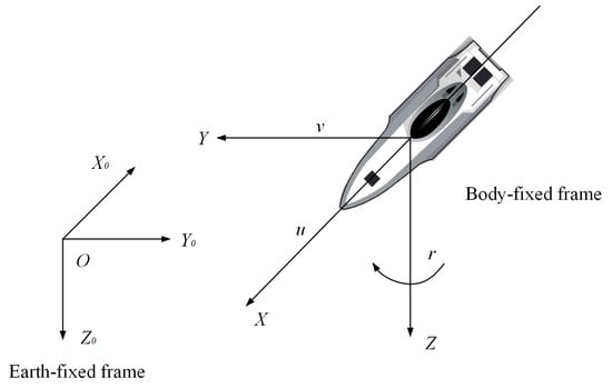
Figure 1.
Graphical illustration of Earth-fixed frame and Body-fixed frame.
Furthermore, denotes the control forces and moments. From a realistic point of view, the propulsion system is physically constrained to provide a limited control force or moment. and can be described as
where indicates the maximum control force or moment provided by vessel propulsion system. is the command control vector calculated by the controller.
Consider the following desired trajectory,
where and denote the desired position and heading angle of the USV, respectively. reflects the desired surge, sway, and yaw angular velocities in the USV body coordinate system. denotes the desired control force and torque.
Assumption 1
([23]). The desired trajectory is smooth, differentiable, and bounded. Both
and are assumed to exist and be bounded.
3. Fixed-Time Precision Tracking with Prescribed Performance Control Scheme
A fixed-time convergence dynamic trajectory tracking control law was developed by integrating the nonsingular terminal sliding mode control, prescribed performance control, and AFISMLDO, which was first proposed to estimate the overall disturbance.
To simplify the controller design, coordinates were transformed as follows:
Integrating Equations (7) and (10), we obtain
where and .
Similarly, according to Equations (9) and (11), we obtain
where and .
The tracking error system can be obtained by subtracting Equation (12) from Equation (13):
where and . denotes the lumped unknown terms containing the unknown system dynamics and external disturbances, which is described as follows:
Assumption 2
([23]). The lumped disturbance is a continuously differentiable function, and its derivative satisfies
and
.
is unknown, bounded, and its maximum upper bound is
.
3.1. Nonlinear Model Transformation
Consider a tracking error system with state variables and subject to the following performance constraints:
where ,, , , , , , and are constants that determine the transient and steady-state responses of the controlled system. The designer can specify the desired response performance according to the task requirements, and prescribed performance control ensures that the system states stay within the preset boundaries. In order to prevent the specified limitations from being broken at the start of control, the following assumption is made before moving forward.
Assumption 3
([30]). The initial conditions of USV satisfy
and
.
The state transformation is defined as
where and are the transformations of variables and , respectively. This transformation guarantees the same monotonicity of the system state before and after the transformation. Therefore, based on this transformation, the required performance of the original system is ensured as long as the converted system is stable.
The derivative of Equation (17) gives
where , ,, and .
Using Equations (14) and (18), we can obtain the following transformed system model:
where , , , , , , , and .
Based on definition , in Equation (17), we can rewrite Equation (19) as
where .
Let and . Then, from Equation (20), we have
where , , , , , , and .
3.2. Adaptive Fixed-Time Lumped Disturbance Observer
To efficiently estimate and correct the lumped disturbances in the system described by Equation (14), we developed a fixed-time lumped disturbance observer that mitigates their impact. By incorporating auxiliary variables into the design of the sliding mode surface, we integrated the fixed-time control theory with the disturbance observer technique to create a lumped disturbance observer with fixed-time convergence performance. This resulted in an accurate estimation of the set total disturbance of the system.
The sliding surface is defined as ,
where is an auxiliary variable and can be expressed as
where is the estimation of .
We then selected the second sliding surface :
where , .
The observer’s derivative is obtained as follows:
where are positive design parameters and , .
Considering Assumption 2, we know that . is subject to adaptive estimation, and the estimated error is defined as follows:
where is the estimation error of and .
Deriving Equations (22) and (24) yields the following expression:
The following inequalities can be deduced from Lemmas 2 and 3:
Similarly, we can obtain
where and are the design parameters.
The sliding mode disturbance observer adaptive law is selected as follows:
Theorem 1.
For the USV trajectory tracking error control system in Equation (14) in the presence of lumped disturbances, if the adaptive law defined in Equation (30) and the adaptive fixed-time lumped disturbance observer defined in Equations (22)–(25) are selected, it is ensured that the overall disturbances are approximated within a fixed time, that is, the estimation error
is confined to a bounded region within a fixed time.
Proof.
To verify Theorem 1, the following candidate Lyapunov function is chosen:
The derivative of Equation (31) is as follows:
By substituting the adaptive law into Equation (30), the inequalities in Equations (28) and (29) are combined into Equation (32). According to Lemma 1, the following inequalities are obtained:
where .
Applying Lemma 5, the parameters are chosen as
Then, Equation (33) is a fixed-time convergence. By selecting the following parameters
, , , and , the convergence time of the fixed-time observer is satisfied as
where . Therefore, the system states converge within a bounded region at a fixed time .
Subsequently, we ascertain the convergence of . Choosing a Lyapunov function and determining its derivative, we have
When parameter is chosen, it is ensured that Equation (35) converges at a fixed time.
Consequently, the state of the system approaches sliding mode at a set time in Equation (24), which can be written as
From Lemma 4, it can be inferred that converges to zero at a fixed time. Consequently, when , the observation error also converges to zero at a fixed time , . Therefore, the overall convergence time of the designed AFISMLDO includes both the sliding mode arrival time and the sliding mode moving time and can be expressed as . Using Equation (36) and Lemma 4, the mathematical expression for can be obtained as
☐
Remark 1.
The fixed-time convergence of the lumped disturbance observer is ensured by the integration term in Equation (24). Additionally, including the sign function inside the integral term of the disturbance observer can significantly reduce the jitter phenomena observed in the sliding mode method.
Figure 2 shows a block diagram of the proposed control scheme.
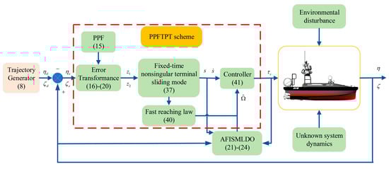
Figure 2.
Schematic of unmanned surface vessel (USV) fixed-time precision tracking control. PPF, prescribed performance function; PPFTPT, prescribed performance fixed-time precision tracking; AFISMLDO, adaptive fixed-time integral sliding mode lumped disturbance observer.
3.3. Controller Design and Stability Analysis
For fixed-time control technique, faster transient response results in greater control force or moment to drive USV to track the preset trajectory. Therefore, thruster saturation is more likely to occur. To alleviate the input saturation problem, the following adaptive auxiliary system is designed [23]:
where and are auxiliary variables. and are appropriate parameter matrices. is the difference between the command control input and the actual control input.
A fixed-time nonsingular terminal sliding mode is constructed for variables and as follows:
where , , , ,. can be given by the following equation:
where is a minimal positive number, , , and satisfy the following equations:
The time derivative of (39) is given as
where .
In order to improve the convergence speed of sliding mode variables and suppress chattering, a fixed-time reaching law based on arctangent function is designed as follows:
where , , , . and are positive odd number and . .
Combining Equations (21)~(43), the PPFTPT control strategy is designed as follows:
Theorem 2.
For the system described in Equation (21), under Assumptions 1–3, the PPFTPT control scheme in Equation (44) ensures that the USV follows the desired trajectory rapidly and precisely while meeting the transient and steady-state responses. It ensures that the actual position and velocity errors of the USV are stabilized within a small neighborhood of the equilibrium point in a fixed time, and the convergence time is independent of the system’s initial state. The convergence time
, and
. where and are positive constants,
,
.
Proof.
The proof of Theorem 2 consists of two phases: the sliding mode arrival phase and the sliding phase.
Step 1. We select the following Lyapunov function:
Differentiating Equation (45) yields
Substituting Equation (21) into Equation (46),
Substituting the control strategy in Equation (44) into Equation (47),
In the light of Lemma 6, and can reach the sliding surface in a fixed time, and the convergence time satisfies
Step 2. When the sliding mode attains the sliding surface, we have
From Equations (38) and (50), we can obtain
When , the analysis is divided into two cases, namely .
- (1)
- When substituting Equation (39) into Equation (51), the following can be obtained:
That is, Equation (52) satisfies
According to Lemma 4, it can be seen that System (53) is stable in a fixed time, and the convergence time of the system satisfies
- (2)
- When , the following can also be obtained:
Similarly, System (55) is stable in .
In summary, the proposed PPFTPT control scheme based on an adaptive integral sliding mode lumped observer, prescribed performance control, and fixed-time control can enable dynamic error system Equation (21) to be fixed-time stable with a maximum upper bound on the convergence time .
☐
Remark 2.
From Lemma 5, it is clear that the system in Equation (21) is fixed-time stable because the transformation used to obtain this system ensures the same monotonicity of the system state before and after transformation. Therefore, based on this transformation, the predetermined performance of the original system is ensured as long as the transformed system is stable.
4. Simulation Results
Table 1 presents the model parameters for the Cybership II USV created by the Norwegian University of Science and Technology, which was utilized for simulation verification to assess the effectiveness of the proposed PPFTPT control system in terms of accuracy and speed.

Table 1.
Hydrodynamic parameters of the Cybership Ⅱ.
The wind, wave, and current disturbances acting on the USV are assumed to be as follows:
The control input for the desired trajectory is set to .
The initial position and velocity of the desired trajectory are set to and , respectively. The initial state of the USV is set to and .
The observer parameters are , , , and .
The prescribed performance control parameters are , , , , , . The controller parameters are , , , , , and . The maximum values of force and moment of the propulsion system are set to . Auxiliary system parameter matrix .
Additionally, the nonsingular fixed-time sliding mode (NFTSM) control scheme developed by Zhang et al. [21] and the finite-time control (FTC) scheme presented by Wang et al. [15] were selected for comparison to evaluate the performance of the proposed scheme. The relevant parameters were selected to be consistent with the original literature.
Figure 3 depicts the trajectory diagram of USV tracking, a predefined trajectory driven by three different control strategies. The PPFTPT approach developed in this study achieves quicker and more precise tracking while ensuring that the initial steady-state and transient responses of the system satisfy the preset requirements. Figure 4 and Figure 5 show the tracking error curves of the USV for the desired positions and velocities, respectively, of the three control schemes. The curve of rose red color represent the prescribed performance constraint. The findings demonstrate that the proposed PPFTPT scheme ensures the rapid convergence of the tracking error to the equilibrium point and obtains an instantaneous response with a smaller error overshoot, even under the dual influence of complex ocean disturbances and unknown system dynamics. By contrast, the convergence performance of the FTC scheme is affected by the initial state of the system. When the states are away from equilibrium and in a state of iterative correction, the tracking error is significant. The NFTSM control scheme can converge in a fixed time; however, it cannot guarantee the transient and steady-state responses of the system and has a large error overshoot.
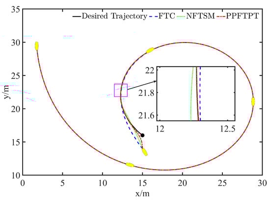
Figure 3.
Trajectory tracking curves. FTC, finite-time control scheme; NFTSM, nonsingular fixed-time sliding mode control scheme.
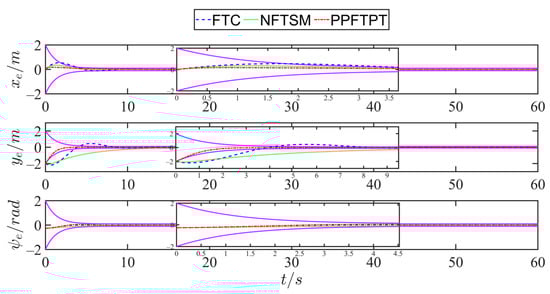
Figure 4.
Position error tracking curves.
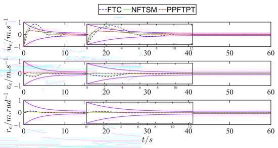
Figure 5.
Velocity error tracking curves.
Figure 6 displays the observation curves of the designed adaptive fixed-time lumped disturbance observer. As demonstrated, compared to the finite-time disturbance observer (FDO) proposed by Wang et al. [15], the AFISMLDO designed in this study accurately reconstructs and compensates for the lumped nonlinearity of the system and converges in a fixed time. Additionally, the presence of a symbolic function within the integral term of the interference observer effectively attenuates the jitter phenomenon in the sliding mode algorithm. Figure 7 shows the control input curve for a suitable control gain. It can be seen from the figure that control input in the initial stage of tracking does not exceed the maximum limit value under the action of the auxiliary system.
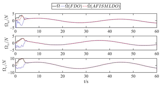
Figure 6.
Observation results of the finite-time disturbance observer (FDO) and AFISMLDO.
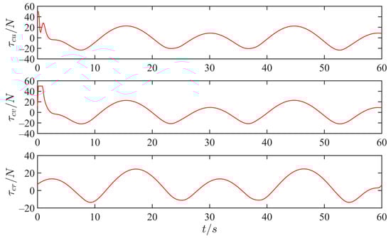
Figure 7.
Control input curves.
In addition, the control performance of the three control schemes was evaluated using two performance indicators: the absolute error integration criterion, , and the time-multiplied absolute error integration criterion, . These are mathematically expressed as follows:
As shown in Table 2 and Table 3, the PPFTPT control strategy presented in this paper achieves the best index values and obtains the highest transient and steady-state accuracy in the presence of unknown dynamic characteristics of the system and complex external disturbances. In summary, the PPFTPT control strategy suggested in this paper can ensure that the USV completes accurate tracking of the desired trajectory and significantly improves the convergence speed and steady-state accuracy of the USV tracking control system.
Table 2.
Integrated absolute errors (IAEs) of the three control schemes.
Table 3.
Integrated time absolute errors (ITAEs) of the three control schemes.
To further verify the fixed-time preset performance convergence characteristics of the established PPFTPT scheme, three different initial states were set for the simulation study, and the initial state configurations are listed in Table 4. The relevant parameters were selected as in previous experiments. As shown in Figure 8, for the three different initial states, the PPFTPT control strategy successfully drove the USV to track the predetermined trajectory almost simultaneously and accurately, and the relative motion states were maintained within the range set by the preset performance function during the entire tracking process. Figure 9 and Figure 10 show the variation curves of the USV position- and velocity-tracking errors, respectively, using the PPFTPT strategy. The results show that the position- and velocity-tracking errors always converged to the equilibrium point quickly within a fixed upper time bound T. Therefore, the influence of the initial state on the tracking performance of the controller was significantly reduced.
Table 4.
Initial position and velocity.
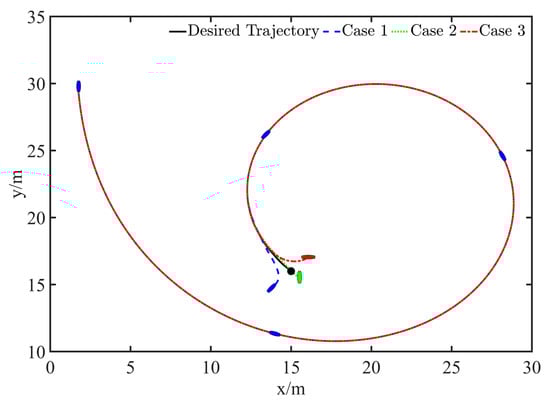
Figure 8.
Trajectory tracking curves under three initial states with PPFTPT scheme.
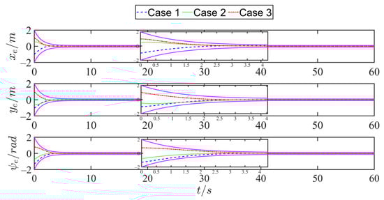
Figure 9.
Position error tracking curves under three initial states with PPFTPT scheme.
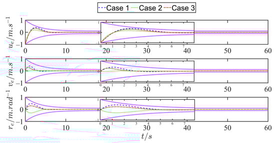
Figure 10.
Velocity error tracking curves under three initial states with PPFTPT scheme.
5. Conclusions
In this study, a novel prescribed performance fixed-time sliding mode control method was proposed to improve trajectory tracking of USVs within an expected time. An adaptive fixed-time lumped disturbance observer was developed to approximate the unknown environmental disturbances and system uncertainties, enhance the robustness and immunity of the control system, and achieve fixed-time convergence of the estimation errors. Subsequently, a PPFTPT control scheme was introduced with a prescribed performance function to enforce a full-state constraint on the system. The control scheme ensures the transient and steady-state responses of the system, eliminates the singularity potential, and achieves the fixed-time convergence of the system, independent of the initial state. Finally, simulation experiments were conducted using the Cybership II ship model, and a comparative analysis of the experimental results verified that the proposed PPFTPT scheme can accurately and quickly track the intended trajectory with a convergence time independent of the initial state of the system. Compared to traditional trajectory tracking methods, the proposed PPFTPT scheme in this study can achieve higher tracking accuracy and stronger robustness and can be stable in fixed time, which is more advantageous in practical applications. However, this study only investigates the trajectory tracking of a single USV, and in the future, we aim to study the cooperative formation tracking control of multiple USVs.
Author Contributions
B.S.: Conceptualization, Methodology, Software, Validation, Writing—original draft, Writing—review and editing. J.Z.: Conceptualization, Methodology, Validation, Writing—review and editing, Supervision. Y.L. (Yan Li): Conceptualization, Writing—review and editing, Supervision. Y.L. (Yiping Liu): Conceptualization, Writing—review and editing, Supervision. Y.Z.: Writing—review and editing. All authors have read and agreed to the published version of the manuscript.
Funding
This work was supported by the National Natural Science Foundation of P.R. China (grant number 51679247) and the Natural Science Foundation of Hubei Province (grant number 2018CFC865). The funders had no role in the study design; in the collection, analysis or interpretation of data; in the writing of the report; or in the decision to submit the article for publication.
Institutional Review Board Statement
Not applicable.
Informed Consent Statement
Not applicable.
Data Availability Statement
Data will be made available upon request.
Conflicts of Interest
The authors declare that they have no known competing financial interests or personal relationships that could have appeared to influence the work reported in this paper.
References
- Sun, X.J.; Wang, G.F.; Fan, Y.S. Trajectory tracking control for vector propulsion unmanned surface vehicle with incomplete underactuated inputs. IEEE J. Ocean. Eng. 2023, 48, 80–92. [Google Scholar] [CrossRef]
- Li, M.Y.; Xu, J.; Xie, W.B.; Wang, H. Finite-time composite learning control for trajectory tracking of dynamic positioning vessels. Ocean Eng. 2022, 262, 112288. [Google Scholar] [CrossRef]
- Qin, H.D.; Chen, X.Y.; Sun, Y.C. Adaptive state-constrained trajectory tracking control of unmanned surface vessel with actuator saturation based on RBFNN and tan-type barrier Lyapunov function. Ocean Eng. 2022, 253, 110966. [Google Scholar] [CrossRef]
- Del-Rio-Rivera, F.; Ramirez-Rivera, V.M.; Donaire, A.; Ferguson, J. Robust trajectory tracking control for fully actuated marine surface vehicle. IEEE Access 2020, 8, 223897–223904. [Google Scholar] [CrossRef]
- Wang, S.T.; Yin, X.H.; Li, P.; Zhang, M.; Wang, X. Trajectory tracking control for mobile robots using reinforcement learning and PID. Iran. J. Sci. Technol. Trans. Electr. Eng. 2020, 44, 1059–1068. [Google Scholar] [CrossRef]
- Alshammari, O.; Mahyuddin, M.N.; Jerbi, H. An advanced PID based control technique with adaptive parameter scheduling for a nonlinear CSTR plant. IEEE Access 2019, 7, 158085–158094. [Google Scholar] [CrossRef]
- Wang, C.X.; Xie, S.R.; Chen, H.; Peng, Y.; Zhang, D. A decoupling controller by hierarchical backstepping method for straight-line tracking of unmanned surface vehicle. Syst. Sci. Control Eng. 2019, 7, 379–388. [Google Scholar] [CrossRef]
- Xu, D.H.; Liu, Z.P.; Zhou, X.Q.; Yang, L.; Huang, L. Trajectory tracking of underactuated unmanned surface vessels: Non-singular terminal sliding control with nonlinear disturbance observer. Appl. Sci. 2022, 12, 3004. [Google Scholar] [CrossRef]
- Kchaou, M.; Jerbi, H.; Ben Ali, N.; Alsaif, H. H∞ Reliable Dynamic Output-Feedback Controller Design for Discrete-Time Singular Systems with Sensor Saturation. Actuators 2021, 10, 196. [Google Scholar] [CrossRef]
- Kchaou, M.; Jerbi, H.; Abassi, R.; VijiPriya, J.; Hmidi, F.; Kouzou, A. Passivity-based asynchronous fault-tolerant control for nonlinear discrete-time singular markovian jump systems: A sliding-mode approach. Eur. J. Control. 2021, 60, 95–113. [Google Scholar] [CrossRef]
- Han, X.; Zhang, X.K. Tracking control of ship at sea based on MPC with virtual ship bunch under Frenet frame. Ocean Eng. 2022, 247, 110737. [Google Scholar] [CrossRef]
- Martinsen, A.B.; Lekkas, A.M.; Gros, S. Reinforcement learning-based NMPC for tracking control of ASVs: Theory and experiments. Control Eng. Pract. 2022, 120, 105024. [Google Scholar] [CrossRef]
- Xu, D.H.; Liu, Z.P.; Song, J.Z.; Zhou, X. Finite time trajectory tracking with full-state feedback of underactuated unmanned surface vessel based on nonsingular fast terminal sliding mode. J. Mar. Sci. Eng. 2022, 10, 1845. [Google Scholar] [CrossRef]
- Huang, D.Q.; Huang, T.P.; Qin, N.; Li, Y.; Yang, Y. Finite-time control for a UAV system based on finite-time disturbance observer. Aerosp. Sci. Technol. 2022, 129, 107825. [Google Scholar] [CrossRef]
- Wang, N.; Karimi, H.R.; Su, S. Accurate trajectory tracking of disturbed surface vehicles: A finite-time control approach. IEEE-ASME Trans. Mechatron. 2019, 24, 1064–1074. [Google Scholar] [CrossRef]
- Zhang, Q.; Zhang, M.J.; Yang, R.; Im, N. Adaptive neural finite-time trajectory tracking control of MSVs subject to uncertainties. Int. J. Control Autom. Syst. 2021, 19, 2238–2250. [Google Scholar] [CrossRef]
- Wang, N.; Gao, Y.; Yang, C.; Zhang, X. Reinforcement learning-based finite-time tracking control of an unknown unmanned surface vehicle with input constraints. Neurocomputing 2022, 484, 26–37. [Google Scholar] [CrossRef]
- Polyakov, A. Nonlinear feedback design for fixed-time stabilization of linear control systems. IEEE Trans. Autom. Control 2012, 57, 2106–2110. [Google Scholar] [CrossRef]
- Yao, Q.J. Fixed-time trajectory tracking control for unmanned surface vessels in the presence of model uncertainties and external disturbances. Int. J. Control 2022, 95, 1133–1143. [Google Scholar] [CrossRef]
- Zhang, J.; Yu, S.; Yan, Y. Fixed-time velocity-free sliding mode tracking control for marine surface vessels with uncertainties and unknown actuator faults. Ocean Eng. 2020, 201, 107107. [Google Scholar] [CrossRef]
- Zhang, J.Q.; Yu, S.H.; Wu, D.F.; Yan, Y. Nonsingular fixed-time terminal sliding mode trajectory tracking control for marine surface vessels with anti-disturbances. Ocean Eng. 2020, 217, 108158. [Google Scholar] [CrossRef]
- Bechlioulis, C.P.; Rovithakis, G.A. Robust adaptive control of feedback linearizable MIMO nonlinear systems with prescribed performance. IEEE Trans. Automat. Contr. 2008, 53, 2090–2099. [Google Scholar] [CrossRef]
- Shen, Z.P.; Wang, Q.; Dong, S.; Yu, H. Prescribed performance dynamic surface control for trajectory-tracking of unmanned surface vessel with input saturation. Appl. Ocean Res. 2021, 113, 102736. [Google Scholar] [CrossRef]
- Ma, Y.F.; He, S.D.; Dong, C.; Dai, S. Finite-time trajectory tracking control of MSV with prescribed transient performance. In Proceedings of the Chinese Control Conference, Guangzhou, China, 27–30 July 2019. [Google Scholar] [CrossRef]
- Zuo, Z.Y. Nonsingular fixed-time consensus tracking for second-order multi-agent networks. Automatica 2015, 54, 305–309. [Google Scholar] [CrossRef]
- Yang, H.J.; Ye, D. Adaptive fixed-time bipartite tracking consensus control for unknown nonlinear multi-agent systems: An information classification mechanism. Inf. Sci. 2018, 459, 238–254. [Google Scholar] [CrossRef]
- Su, B.; Wang, H.B.; Wang, Y.L. Dynamic event-triggered formation control for AUVs with fixed-time integral sliding mode disturbance observer. Ocean Eng. 2021, 240, 109893. [Google Scholar] [CrossRef]
- Qin, H.D.; Si, J.S.; Wang, N.; Gao, L. Fast fixed-time nonsingular terminal sliding-mode formation control for autonomous underwater vehicles based on a disturbance observer. Ocean Eng. 2023, 270, 113423. [Google Scholar] [CrossRef]
- Huang, Y.; Jia, Y. Fixed-time consensus tracking control for second-order multi-agent systems with bounded input uncertainties via NFFTSM. IET Control Theory A 2017, 11, 2900–2909. [Google Scholar] [CrossRef]
- Li, J.; Xiang, X.; Dong, D. Prescribed time observer based trajectory tracking control of autonomous underwater vehicle with tracking error constraints. Ocean Eng. 2023, 274, 114018. [Google Scholar] [CrossRef]
Disclaimer/Publisher’s Note: The statements, opinions and data contained in all publications are solely those of the individual author(s) and contributor(s) and not of MDPI and/or the editor(s). MDPI and/or the editor(s) disclaim responsibility for any injury to people or property resulting from any ideas, methods, instructions or products referred to in the content. |
© 2023 by the authors. Licensee MDPI, Basel, Switzerland. This article is an open access article distributed under the terms and conditions of the Creative Commons Attribution (CC BY) license (https://creativecommons.org/licenses/by/4.0/).