Characterization of Low-Latency Next-Generation eVTOL Communications: From Channel Modeling to Performance Evaluation

Abstract

Next-generation wireless communication networks are expected to offer extremely high data rates supported by very low latency and radically new applications, which require a new wireless radio technology paradigm. However, it is crucial to assist the radio link over the fast varying and highly dynamic channel to satisfy the diverse requirements of next-generation wireless networks. Recently, communication via autonomous electric vertical takeoff and landing (eVTOL) has gained momentum, owing to its potential for cost-effective network deployment. It is considered one of the most promising technologies conceived to support smart radio terminals. However, to provide efficient and reliable communications between ground base stations and eVTOLs as well as between eVTOLs and other eVTOLs, realistic eVTOL channel models are indispensable. In this paper, we propose a nonstationary geometry-based stochastic channel model for eVTOL communication links. The proposed eVTOL channel model framework considers time-domain nonstationarity and arbitrary eVTOL trajectory and is sufficiently general to support versatile C bands. One of the critical challenges for eVTOL is the fast vertical takeoff and landing flight patterns affecting the regular propagation communication channel. Moreover, we present a new method for estimating the SNR over the non-stationary fast dynamic time-variant eVTOL channel by utilizing the sliding window adaptive filtering technique. Furthermore, we present an information–theoretic approach to characterize the end-to-end transmission delay over the eVTOL channel and prove that the optimal transmission scheme strongly depends upon the eVTOL link configuration. In addition, to analyze the occurrence of deep fade regions in eVTOL links, we analyze the outage probability, which is an important performance metric for wireless channels operating over dynamic fading channels, and make an important observation that the outage probability increases non-linearly with the eVTOL height. Furthermore, we consider the commercially available eVTOL specifications and data to validate the channel model and analyze the Doppler shift and latency for the exponential acceleration and exponential deceleration velocities profiles during the takeoff and landing operation. This paper provides a new and practical approach for the design, optimization, and performance evaluation of future eVTOL-assisted next-generation wireless communications.

1. Introduction

With the recent progress beyond 5G and 6G wireless technology, ultra-reliable and low-latency communications (URLLC) have attracted much attention due to their potential applications in automated driving, vehicular-to-vehicular communications, and factory automation [1]. Recently, along with unmanned aerial vehicles (UAVs), there has been a significant growth in the use of flying cars and electric vertical takeoff and landings (eVTOLs) to significantly reduce traffic congestion. It is well known that the space–air–ground integrated network (SAGIN) will be one of the key technologies for next-generation wireless systems [2]. It is reported that the autonomous air vehicle communication system will play a critical role in building the SAGIN [3].

While autonomous air vehicles, UAVs, and eVTOLs could eventually become one of the defining killer apps for the next-generation wireless systems, they exhibit unprecedented command and control, as well as connectivity requirements, in a 3D propagation environment. Due to the high possibility of continuous severe fading over the eVTOL channel, the delay violation is inevitable [4]. Moreover, unlike conventional ground-to-ground (G2G) or base-station-to-ground (B2G) communications, communication links involving aerial vehicles have different physical characteristics.

There have been studies showing eVTOL with multiple modes of applications, including connectivity to meet the platform data service requirements. Proper processes have to be chosen to meet each application system’s characteristics. To increase the reliability to meet the Quality of Service (QoS) requirements, the reliability and latency have to be optimized. In addition, the standard provided coding methods must be part of the protocol. The Low-Density Parity-Check (LDPC) code was adapted by the 3rd Generation Partnership Project Organization (3GPP). The tradeoff between the ULL speed and bandwidth shows the results of meeting these criteria. A short description about the few wireless channel models are presented in Table 1.

1.1. Background and Motivation

It is worth mentioning that, since eVTOL is newly emerging, it has not been explored much from the communication perspective. Moreover, the few studies that have been conducted on eVTOL and UAV channel modeling are still in their infancy. In general, the channel models can be broadly categorized into stochastic and deterministic models. A deterministic aerial channel model based on the finite difference time-domain method was proposed for UAV [5]. However, the deterministic channel models have their limitations, as they need a very detailed description of a location or site-specific channel environment to predict the propagation behavior and, therefore, require a large amount of computation time. Conversely, in the stochastic channel models, the propagation parameters are represented in a probabilistic manner and can, therefore, adapt to various scenarios. Stochastic channel models can be further divided into geometric-based stochastic models and non-geometrical stochastic models.

A non-geometric-based narrowband channel model for UAV-to-ground communication was presented in [6]. The authors characterized the channel model without assuming any scattering geometry. Moreover, they also ignored the very fundamental property of the UAV channel, which is time non-stationarity. Recently, a few studies have been conducted considering the time non-stationarity of the UAV channel environment. For instance, a space-time non-stationary geometric-based stochastic channel model for 6G massive multiple-input multiple-output (MIMO) mmWave UAV communication was proposed [7]. The authors considered the impact of the moving speed, altitude, and moving direction on the performance evaluation. In another similar study, considering a UAV-to-ground wireless channel, a non-stationary channel model was proposed [8]. In particular, a 3D non-stationary geometric-based stochastic channel model for UAV-to-ground MIMO links was obtained. The model was generic to multiple frequency bands, including mmWave. The statistical properties, including the delay spread and the power delay profile, were analyzed for various channel conditions and frequencies. With a similar objective, a 3D non-stationary channel model for UAV-to-ground communication MIMO link was obtained [9]. In particular, an angular estimation algorithm was developed to estimate the real-time azimuth angle of departure, the elevation angle of departure, the azimuth angle of arrival, and the elevation angle of arrival. The following important channel models, based on the 3GPP, standards are illustrated in Table 1. Further, in addition to the enhancement of performance brought by the accuracy in channel modeling, some research has further used channel model and key performance indicators (KPIs) obtained from outdoor experiments for UAV positioning [10], which have significant impacts on UAV applications in critical verticals. Recently, a comprehensive analysis on low latency UAV communication was documented [11]. The authors obtained the capacity bound for the UAV channel and presented the information–theoretic-based framework to analyze the latency over different link geometries.

Table 1. Next-generation wireless channel models.

Channel Model	Application	Description
3D Channel [12]	WINNER II/WINNER +	3GPP concept with altitude taken into account to fill in the gaps of 2D channel modles
3D Channel on outdoor urban [13]	Urban microcells (UMi) and urban macrocells	Various measurement activities in different frequency bands and scenarios at Aalborg, Denmark
5G Millimeter-Wave Bands [14]	Model of mmWave up to 100 GHz	Compared channel data with NYUSIM model to show channel efficiency and multipath effects

Table 1. Next-generation wireless channel models.

Channel Model	Application	Description
3D Channel [12]	WINNER II/WINNER +	3GPP concept with altitude taken into account to fill in the gaps of 2D channel modles
3D Channel on outdoor urban [13]	Urban microcells (UMi) and urban macrocells	Various measurement activities in different frequency bands and scenarios at Aalborg, Denmark
5G Millimeter-Wave Bands [14]	Model of mmWave up to 100 GHz	Compared channel data with NYUSIM model to show channel efficiency and multipath effects

1.2. Contributions

The design of a next-generation wireless system with an eVTOL communication link requires knowledge about the propagation characteristics in which the envisioned system will operate. A key characteristic of the eVTOL channel is its temporal variability and inherent non-stationarity, which has a major impact on the reliability constraint and latency. However, to the best of the authors’ knowledge, no detailed investigations have been conducted in modeling and characterizing the eVTOL communication channel. Motivated by this, in this article, we characterized the eVTOL channel and subsequently conducted a performance analysis in terms of latency and outrage probability. The main contributions of this paper are listed below:

• We develop a channel model for wireless links in eVTOL communications, which include BS-to-eVTOL and eVTOL-to-eVTOL channels. In characterizing the non-stationary eVTOL channel, we consider the eVTOL moving direction, link configuration, and the speed of the eVTOL;
• We present a new method for estimating the SNR over a fast time-variant dynamic eVTOL channel by utilizing the sliding window adaptive filtering technique with the least mean square approach;
• The fading distribution that describes the widest range of fading behavior exhibited by the non-stationary eVTOL communication channel is derived. It is anticipated that the PDF presented in this paper is valuable for estimating the performance of the modern eVTOL communication links, either through computer simulations or analytically;
• We develop an optimization framework to minimize ground-to-eVTOL and eVTOL-to-eVTOL communication costs while ensuring quality-of-service constraints such as communication link capacity, reliability, and end-to-end transmission delay;
• Subsequently, we consider the commercially available eVTOL specifications and data to validate the channel model and analyze the Doppler shift and latency for the exponential acceleration and exponential deceleration velocity profiles during the takeoff and landing operation;
• Due to the non-stationary dynamic channel of the eVTOL link, it is critical to analyze the occurrence of an outage due to the fall of the SNR below the respective predetermined threshold. To this end, we analyze the outage probability and make an important observation that the outage probability increases non-linearly with the eVTOL height. It is an important performance observation for eVTOL links operating over dynamic fading conditions to identify the deep fade regions.

2. System Model and Channel Characterization

The system model under consideration is illustrated in Figure 1.

The complex channel impulse response between the moving source x and the moving destination y can be represented by the superposition of the LOS and NLOS components as follows [7]:

$$h\left(t,\tau \right)=\sqrt{\frac{K}{K+1}}{h}_{xy}^{LOS}\left(t,\tau \right)+\sqrt{\frac{1}{K+1}}{h}_{xy}^{NLOS}\left(t,\tau \right),$$

(1)

where $h_{xy}^{LOS}\left(t,\tau \right)$ can be modeled as shown:

$$\begin{array}{cc}\hfill & h_{xy}^{LOS}\left(t,\tau \right)={\left[\begin{array}{c}{A}_y^V\left({\theta }_{E,y}^{LOS},{\theta }_{A,y}^{LOS}\right)\\ A_y^H\left({\theta }_{E,y}^{LOS},{\theta }_{A,y}^{LOS}\right)\end{array}\right]}^T\left[\begin{array}{cc}exp\left(j{\varphi }_V^{LOS}\right)& 0\\ 0& exp\left(j{\varphi }_H^{LOS}\right)\end{array}\right]\left[\begin{array}{c}{A}_x^V\left({\theta }_{E,x}^{LOS},{\theta }_{A,x}^{LOS}\right)\\ A_x^H\left({\theta }_{E,x}^{LOS},{\theta }_{A,x}^{LOS}\right)\end{array}\right]\hfill \\ \hfill & \times exp\left(2\pi f_c{\tau }_{xy}^{LOS}\left(t\right)\delta \left(\tau -{\tau }_{xy}^{LOS}\left(t\right)\right)\right),\hfill \end{array}$$

(2)

whereas $h_{xy}^{NLOS}\left(t,\tau \right)$ can be modeled as below:

$$\begin{array}{cc}\hfill & h_{xy}^{NLOS}\left(t,\tau \right)=\hfill \\ \hfill & \sum _{r=1}^{R_{xy}\left(t\right)}\left\{\sum _{m_r=1}^{M_r}\left\{{\left[\begin{array}{c}{A}_y^V\left({\theta }_{E,y}^{m_r},{\theta }_{A,y}^{m_r}\right)\\ A_y^H\left({\theta }_{E,y}^{m_r},{\theta }_{A,y}^{m_r}\right)\end{array}\right]}^T\left[\begin{array}{cc}exp\left(j{\varphi }_V^{m_r}\right)& \sqrt{{\Theta }_{m_r}^{-1}}exp\left(j{\varphi }_{VH}^{m_r}\right)\\ \sqrt{{\Theta }_{m_r}^{-1}}exp\left(j{\varphi }_{HV}^{m_r}\right)& exp\left(j{\varphi }_H^{m_r}\right)\end{array}\right]\right.\right.\hfill \\ \hfill & \left.\left.\times \left[\begin{array}{c}\sqrt{P_x^{m_r}\left(t\right)}{A}_x^V\left({\theta }_{E,x}^{m_r},{\theta }_{A,x}^{m_r}\right)\\ \sqrt{P_x^{m_r}\left(t\right)}{A}_x^H\left({\theta }_{E,x}^{m_r},{\theta }_{A,x}^{m_r}\right)\end{array}\right]exp\left(2\pi f_c{\tau }_{xy}^{m_r}\left(t\right)\delta \left(\tau -{\tau }_{xy}^{m_r}\left(t\right)\right)\right)\right\}\right\}.\hfill \end{array}$$

(3)

The description about the system’s parameters are listed in

Table 2. System parameters.

Parameter	Description
K	K-factor
$f_c$	Carrier frequency
$A_x^V\left(A_x^H\right)$	Source antenna pattern for vertical (horizontal) polarization
$A_y^V\left(A_y^H\right)$	Receiver antenna pattern for vertical (horizontal) polarization
${\theta }_{E,x}^{LOS}\left({\theta }_{A,x}^{LOS}\right)$	Elevation (azimuth) angle of departure of the LOS component
${\theta }_{E,y}^{LOS}\left({\theta }_{A,y}^{LOS}\right)$	Elevation (azimuth) angle of arrival of the LOS component
$R_{xy}\left(t\right)$	Total number of paths at time instant t for NLOS link
$A_F^r$	Attenuation of the rth path
$v_x$	Velocity of the transmitter x
$v_y$	Velocity of the receiver y
v	Relative velocity between the transmitter and the receiver
${\Theta }_{m_r}$	Cross-polarization power ratio
$M_r$	Number of rays in the rth path
$N_s$	Number of samples
$w\left(n\right)$	Gaussian noise at time index n
${\sigma }_{NLOS}^2$	Variance of the NLOS fading components
$\delta$	Step size
$N_c$	Length of the codeword
$P_x$	Transmit power
$T_b$	Bit duration
$d_{xy}$	Distance between the transmitter x and the receiver y

.

2.1. Base-Station-to-eVTOL (B2E) and eVTOL-to-eVTOL (E2E) Link Characteristics

Utilizing (1), (2), and (3), the narrowband process corresponding to the rth propagation path can be represented as follows:

$$\begin{array}{cc}\hfill & h_{xy}^r\left(t\right)=A_F^{r}exp\left[j\left({\varphi }_0-2\pi f_c{\tau }_{xy}^r\left(t\right)\right)\right]\hfill \\ \hfill & \times exp\left[j\frac{2\pi }{\lambda }{v}_{x}tcos\left({\theta }_{A,x}^r-{\theta }_{V,x}\right)cos\left({\theta }_{E,x}^r-{\theta }_{H,x}\right)\right]\hfill \\ \hfill & \times exp\left[j\frac{2\pi }{\lambda }{v}_{y}tcos\left({\theta }_{A,y}^r-{\theta }_{V,y}\right)cos\left({\theta }_{E,y}^r-{\theta }_{H,y}\right)\right].\hfill \end{array}$$

(4)

The representation in (4) accounts for the fact that the overall channel response can be interpreted as a sum of the specular component and the diffused nonspecular components. Furthermore, the in-phase and the quadrature portions of the diffuse component are due to the sum of a large number of small and independently distributed phased waves [15]. $A_F^r\in \mathbb{C}$ denotes the attenuation of path r. $v_x$ and $v_y$ represent the velocities of the transmitter and the receiver, respectively.

Due to the time-variant channel conditions, we considered block-oriented transmission, so that the eVTOL communication system can adapt to the changing channel conditions and can, therefore, optimize the transmission for each block. With sampled time-variant discrete-time channel $h_{xy}\left[n_c\right]\triangleq h_{xy}(n_c{T}_s,0)$, the received signal can then be modeled as below:

$$Y\left[n_c\right]=\sqrt{P_x{d}_{xy}^{-\alpha }}{h}_{xy}\left[n_c\right]X\left[n_c\right]+w\left[n_c\right],n_c\in \left\{0,1,···,N_c\right\},$$

(5)

where $P_x$ is the transmit power and $w\left[m\right]\sim \mathcal{CN}(0,{\sigma }_w^2)$ is circular symmetric complex Gaussian distributed white noise with zero mean and variance ${\sigma }_w^2$. d is the distance between the transmitter and the receiver. $\alpha$ denotes the path loss exponent. Utilizing (4), $h_{xy}\left[n_c\right]$ can be obtained in a simplified form:

$$h_{xy}\left[n_c\right]=\sum _{r=1}^{R_{xy}}{A}_F^{r}exp\left(j2\pi f_D^r{T}_s{n}_c\right),$$

(6)

where $f_D^r\in \mathbb{R}$ denotes the Doppler shift of the rth path and is a function of the angle of departure, angle of arrival, velocities of the transmitter and the receiver, and the carrier frequency $f_c$. Moreover, the covariance matrix of the channel over the given block is defined as follows:

$${\Xi }_{h_{xy}}=\mathbb{E}\left[\begin{array}{ccc}{h}_{xy}^2\left[0\right]& ···& h_{xy}\left[0\right]h_{xy}\left[N_c-1\right]\\ ⋮& \ddots & ⋮\\ h_{xy}\left[N_c-1\right]h_{xy}\left[0\right]& \cdots & h_{xy}^2[N_c-1]\end{array}\right].$$

(7)

We point out that the rank of the channel covariance matrix ${\Xi }_{h_{xy}}$ is the minimum of $R_{xy}$ and $N_c$ and can, therefore, be defined as $\mathrm{rank}({\Xi }_{h_{xy}})=\min (R_{xy},N_c)$.

2.2. Fading Characterization for eVTOL Communication Link

Next, we present the framework to obtain the general PDF of the fading envelope of $h_{xy}$. Since $h_{xy}$ is the sum of independent random propagation paths, the PDF of the fading envelope can readily be obtained by using the characteristic function approach [16]. The characteristic function of $h_{xy}^{LOS}$ component is given by $J_0\left(q\sqrt{M_c^2+M_s^2}\right)$, where $J_0(·)$ is the Bessel function of the first kind of order zero. $q\in {\mathbb{R}}^{+}$ is a continuous positive real number such that $0<q<\infty$. $M_c$ and $M_s$ are defined as shown in (8) and (9), respectively:

$$\begin{array}{c}\hfill M_c=A_y^V\left({\theta }_{E,y}^{LOS},{\theta }_{A,y}^{LOS}\right)A_x^V\left({\theta }_{E,x}^{LOS},{\theta }_{A,x}^{LOS}\right)cos\left({\varphi }_V^{LOS}\right)\\ \hfill +A_y^H\left({\theta }_{E,y}^{LOS},{\theta }_{A,y}^{LOS}\right)A_x^H\left({\theta }_{E,x}^{LOS},{\theta }_{A,x}^{LOS}\right)cos\left({\varphi }_H^{LOS}\right),\end{array}$$

(8)

and

$$\begin{array}{c}\hfill M_s=A_y^V\left({\theta }_{E,y}^{LOS},{\theta }_{A,y}^{LOS}\right)A_x^V\left({\theta }_{E,x}^{LOS},{\theta }_{A,x}^{LOS}\right)sin\left({\varphi }_V^{LOS}\right)\\ \hfill +A_y^H\left({\theta }_{E,y}^{LOS},{\theta }_{A,y}^{LOS}\right)A_x^H\left({\theta }_{E,x}^{LOS},{\theta }_{A,x}^{LOS}\right)sin\left({\varphi }_H^{LOS}\right).\end{array}$$

(9)

The characteristic function of the NLOS component is given by $exp\left(\frac{-q^2{\sigma }_{NLOS}^2}{2}\right)$ [17]. Following this, the general form of the envelope PDF can be written:

$$\begin{array}{cc}\hfill & f_{h_{xy}}\left(h_{xy}\right)=\underset{0}{\overset{\infty }{\int }}{h}_{xy}q{J}_0\left(q{h}_{xy}\right)J_0\left(\left|h_{xy}^{LOS}\right|q\right)exp\left(\frac{-q^2{\sigma }_{NLOS}^2}{2}\right)dq.\hfill \end{array}$$

(10)

The integral in (10) is obtained in a closed form, as depicted in (11):

$$f_{h_{xy}}\left(h_{xy}\right)=\sum _{k=0}^{\infty }{\left(-\frac{1}{2}\right)}^k{\left(\frac{1}{k!}\right)}^2\frac{h_{xy}^{2k+1}}{{\sigma }_{NLOS}^{2\left(k+1\right)}}{G}_{1,2}^{1,1}\left[\frac{{\left|h_{xy}^{LOS}\right|}^2}{2{\sigma }_{NLOS}^2}\left|\begin{array}{c}-k\\ 0,0\end{array}\right.\right].$$

(11)

The derivation steps of (11) are illustrated in Appendix A.

Remark 1.

Although the expression for $f_{h_{xy}}\left(h_{xy}\right)$ in (11) is in the form of an infinite series, it converges quickly for finitely small values of the summand k. The convergence is evident from the result depicted in Figure 2. To test the convergence of the (11), we apply the D’Alembert (or Cauchy) Ratio Test and prove that (11) converges quickly with small values of the summand, as shown in Figure 2. The derivation of the D’Alembert (or Cauchy) Ratio Test is illustrated in Appendix B.

Based on the D’Alembert Ratio for (11), as obtained in Appendix B, Figure 2 confirms the convergence of the expression derived in (11). As can be readily seen from the D’Alembert (or Cauchy) Ratio Test in Appendix B, $C_h\le 0<1,\forall k$, thereby satisfying the D’Alembert Ratio Test for convergence.

To measure the dispersion or the spread of the fading values, we plotted (11) for different values of the variance of the diffused components ${\sigma }_{NLOS}^2$, as illustrated in Figure 3. It can be seen that increasing the variance results in a wider spread of the fading channel and a flatter fading distribution. Moreover, a lower ${\sigma }_{NLOS}^2$ results in a higher decay rate, indicating a smaller dynamic range of fading channel and a lower probability of extreme fading events. To simulate (11), about 120 terms are required for summation to achieve accuracy at the 6th significant digit.

The random channel realizations were obtained to analyze the phase and magnitude distribution for the B2E and E2E links over different multipaths. The results presented in Figure 4 and Figure 5 correspond to the phase distributions for the E2E and B2E channel links, respectively. Results indicate that for the E2E link, the angular spread of the channel is lower when compared to that of the B2E link, as can be seen from the phase distribution profiles illustrated in Figure 4 and Figure 5.

Figure 6 and Figure 7 show the received power distributions of the E2E and B2E fading channels, respectively. In obtaining these results, the transmit power was set to 35 dBm. The receiver position was set to $(10,10,75)$ m. For the E2E link, the transmitting eVTOL was located at $(0,0,50)$ m, whereas, for the B2E link, the transmitter position was set to $(0,0,0)$ m. The results reveal a few important observations. They indicate that the B2E link was mainly composed of multipaths with diffused power levels. However, the analysis of E2E links shows that there exists a specular dominating multipath component along with the components with diffused power.

Based on Figure 6 and Figure 7, the statistic distribution views for the received power between B2E and E2E show similarities for the first five significant paths. However, the instant magnitudes array, that includes all five paths at each time stamp, shows a distinct pattern between B2E and E2E.

As shown in Figure 8, the normalized received power arrays of E2E and B2E demonstrate different behaviors in most data samples that could be recognized by unsupervised t-SNE projection. This observation further motivates the distinguished modeling of the B2E and E2E channels.

Further, to validate the argument that the B2E link is mainly composed of the multipath with diffused power levels, Figure 9 illustrates the variance in the received signal samples over different time intervals. In obtaining these results, we considered 50 samples in each interval. The results indicate a higher variance in the signal received over the B2E link when compared to the variance in the signal received over the E2E link. This shows that the multiple paths in the B2E link over different intervals can have a wider range of signal strengths, and, when these multiple copies of the signal arrive at the eVTOL, they can interfere constructively or destructively, leading to highly random variations in the received signal strength when compared to the signal received over the E2E link. As the relative phases and delays of the multipath components vary with time, the resultant signal strength at the eVTOL fluctuates, leading to variations in the observed variance in the fading samples. The different variances observed in each time interval in a B2E fading channel are a manifestation of the random and time-varying nature of multipath propagation, where the combined effects of the multipath components result in fluctuations in the received signal strength.

Figure 10 illustrates the channel characterization. The results indicate that, when compared to that of the E2E link, there is no significant or dominating component or path in the B2E link, and, therefore, the total received signal in the B2E link is a result of the combined effect of multiple diffused random components. Physically, the results can be interpreted as the higher changing level of constructive or destructive interference between the multipath components. Moreover, the results depicted show that, for the B2E links, the signal arrives at the receiver from different directions or angles. This also indicates that these multiple diffused paths have different lengths and may experience different levels of attenuation, phase shifts, and delays. As a result, the received signal at the eVTOL can arrive from different angles, leading to large variations in the angle of arrival in the case of the B2E link. In practical scenarios, large variations in the angle of arrival can have important implications for eVTOL communication systems. Large variations can lead to significant fluctuations in the received signal strength and, thereby, potentially impact the performance of the system. Understanding and characterizing the angle of arrival variations in eVTOL channels is crucial for designing robust eVTOL communication systems that can mitigate the effects of multipath propagation and maintain reliable high-quality wireless connections.

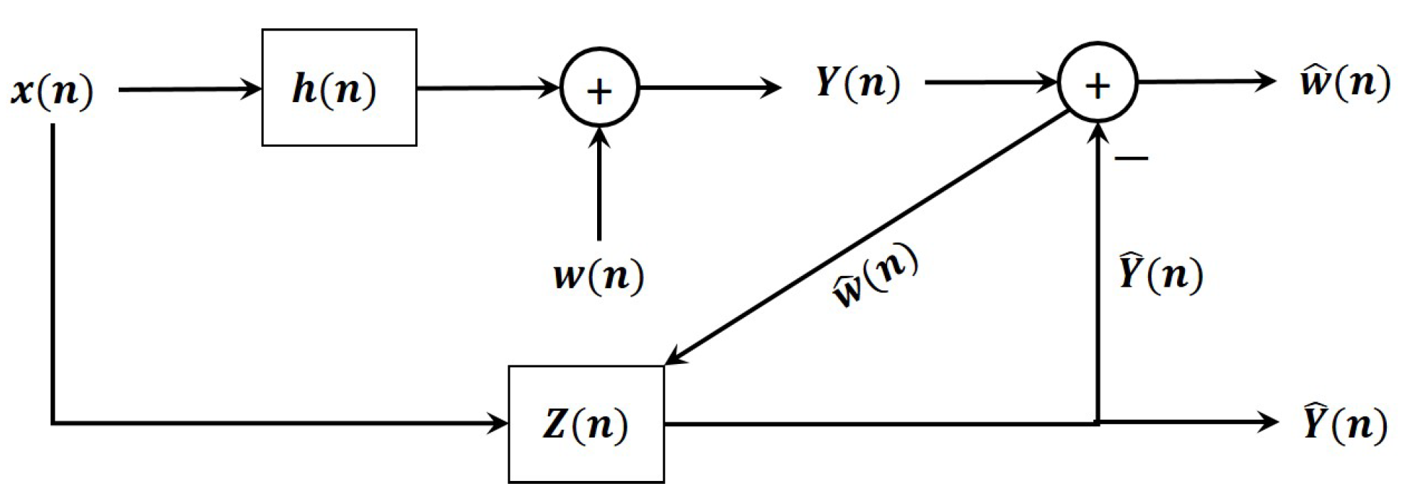
2.3. Noise and SNR Estimation

Due to the non-stationary channel, we approximated the power of a signal by the short-term power average of that signal over the $N_s$ number of samples, such that $N_s>>N_c$, leading to the following:

$$E\left[Y^2\left(n\right)\right]\approx \frac{1}{N_s}\sum _{j=1}^{N_s}{Y}^2\left(n+j\right).$$

(12)

Similarly, the time-variant noise power is approximated as the short-term power of the noise signal $w\left(n\right)$, given by the following:

$$E\left[w^2\left(n\right)\right]\approx \frac{1}{N_s}\sum _{j=1}^{N_s}{w}^2\left(n+j\right).$$

(13)

Following (12) and (13), the SNR at any time index n can be approximately obtained as below:

$$\chi \approx \frac{{\displaystyle \sum _{j=1}^{Ns}}{Y}^2\left(n+j\right)}{{\displaystyle \sum _{j=1}^{N_s}}{w}^2\left(n+j\right)}.$$

(14)

We point out that, due to the time-variant channel characteristics of the BS-to-eVTOL and eVTOL-to-eVTOL, the noise signal $w\left(n\right)$ is difficult to measure in a real system. Therefore, we adopted a normalized least mean square method to estimate the noise signal $w\left(n\right)$. The method to estimate the signal and the noise for the eVTOL communication link is illustrated in Figure 11.

In Figure 11, $\mathbf{Z}\left(n\right)={\left[Z_0\left(n\right),Z_1\left(n\right),···,Z_{N_Z-1}\left(n\right)\right]}^T$ represents the filter of length $N_Z$, whose coefficients can be obtained adaptively using the time-recursive approach:

$$\mathbf{Z}\left(n+1\right)=\mathbf{Z}\left(n\right)+\delta \hat{w}\left(n\right)\frac{\mathbf{x}\left(n\right)}{{\displaystyle \sum _{j=0}^{N_s}}{x}^2\left(n+j\right)},$$

(15)

where $\delta$ denotes the step size and $\mathbf{x}\left(n\right)={\left[x\left(n\right),x(n-1),···,x(n-N_Z+1)\right]}^T$. Utilizing the signals flow diagram in Figure 11 and the definition of $\mathbf{Z}\left(n+1\right)$ provided in (15), the estimation of $w\left(n\right)$ can be written as follows:

$$\hat{w}\left(n\right)=Y\left(n\right)-{\left[\delta {\displaystyle \sum _{j=1}^{N_s}}Y\left(n-j\right)\frac{\mathbf{x}\left(n-j\right)}{{\displaystyle \sum _{j=0}^{N_s}}{x}^2\left(n+j\right)}\right]}^T\mathbf{x}\left(n\right).$$

(16)

2.4. SNR Estimation

Considering the noisy received signal and utilizing (7), (14) and (16), the modified channel covariance matrix is given by the following:

$${\hat{\Xi }}_{h_{xy}}=\mathbb{E}\left[\begin{array}{ccc}{h}_{xy}^2\left[0\right]+\frac{1}{\hat{\chi }}& ···& h_{xy}\left[0\right]h_{xy}\left[N_c-1\right]\\ ⋮& \ddots & ⋮\\ h_{xy}\left[N_c-1\right]h_{xy}\left[0\right]& \cdots & h_{xy}^2[N_c-1]+\frac{1}{\hat{\chi }}\end{array}\right].$$

(17)

It is to be noted that ${\hat{\Xi }}_{h_{xy}}$ takes into account the impact of the noise at the receiver. Expanding the channel into an orthogonal basis function ${\varphi }_j\left[n_c\right],j\in \{0,1,···,Z-1\}$, the channel coefficients can then be written as shown:

$${\hat{h}}_{xy}\left[n_c\right]=\sum _{j=0}^{Z-1}{\varphi }_i\left[n_c\right]b_j\approx h_{xy}\left[n_c\right],$$

(18)

where $b_j$ denotes the basis expansion coefficient that can be estimated as follows:

$$b_j=\sum _{n_c=0}^{N_c-1}{\varphi }_j^{*}\left[n_c\right]{\hat{x}}^{*}\left[n_c\right]Y\left[n_c\right].$$

(19)

Remark 2.

As illustrated in (19), estimating $b_j$ requires the knowledge of $x\left[n_c\right]$.

Figure 12 illustrates the performance of the proposed SNR estimation method. In analyzing the performance of the SNR estimation method, the impulse response was chosen to be random, with samples generated using the distribution derived in (11). In obtaining the results depicted in Figure 12, the Gaussian noise was added to the system response, and the simulation was carried out for two different initial SNR values: −5 dB and 30 dB. Due to the time-variant random fading, the real-time SNR varies, and the results clearly show the significant performance of the proposed SNR estimation approach. They depict that the SNR estimates are very close to the real-time SNR.

The SNR estimation error and the impact of the window size on the proposed method are illustrated in Figure 13, for different values of the true SNR, as shown in Figure 13a,b. The estimation error plots provide useful insights into the accuracy of the proposed method based on the sliding window adaptive filtering technique with the least mean square approach. A few observations made on the basis of the results obtained are listed below:

• The results show that the SNR estimation is relatively accurate with minimal bias. However, occasional spikes in the estimation error indicate instances of higher fading fluctuations;
• It can also be seen that the smaller window size can result in higher spikes in the estimation error. This can be attributed to the limited number of samples used for smoothing, which, in turn, make the estimation error more sensitive to random fluctuations. It can also be concluded that a larger window size can lead to smoother estimation error plots with reduced variations. Therefore, the choice of an appropriate window size depends on the specific requirements of the communication system, balancing the need for accurate estimation and the desired responsiveness to SNR variations.

3. Results and Discussions

In this section, the derived channel characteristics of the eVTOL link are evaluated through simulations and numerically. We investigated the impact of eVTOL link configurations on the received SNR and the fading statistics in terms of the Rician K factor. In addition, the results are provided to analyze the latency and the outage probability. To achieve a good statistical average, 10,000 realizations were generated for a given set of parameters. The empirical estimate of the fading statistics was obtained by averaging the results over 5000 realizations. The Meijer G-function in (11) was implemented in Python using the “mpmath” library. For (11), about 120 terms are required for summation to achieve accuracy at the 6th significant digit. Unless otherwise stated, the simulation parameters are as illustrated in Table 3.

To analyze the shift in the carrier frequency due to the Doppler effect, we considered the following eVTOLs specifications: EHang 216 [18], Wisk Cora [19], and the Joby S4 [20]. We considered the exponential deceleration velocity profile for the eVTOL landing with initial velocities equal to 62 mph, 110 mph, and 165 mph for the three eVTOLs [19]. As illustrated in Figure 14, the results show that different eVTOLs experience different frequency shifts. This information is important in designing efficient eVTOL communication systems and ensuring optimized signal reception.

Table 3. System parameters.

Parameter	Value
$P_m$	35 dBm
Packet size	32 bytes
Rice factor of B2E link	$5\sim 12$ dB
Rice factor of E2E link	$10\sim 12$ dB
Noise spectral density $N_0$ [21]	$-174$ dBm/Hz
LOS (NLOS) shadow fading standard deviation	4 $\left(6\right)$ dB
Carrier frequency $f_c$	$3.5$ GHz (C band)
Window size	50

Table 3. System parameters.

Parameter	Value
$P_m$	35 dBm
Packet size	32 bytes
Rice factor of B2E link	$5\sim 12$ dB
Rice factor of E2E link	$10\sim 12$ dB
Noise spectral density $N_0$ [21]	$-174$ dBm/Hz
LOS (NLOS) shadow fading standard deviation	4 $\left(6\right)$ dB
Carrier frequency $f_c$	$3.5$ GHz (C band)
Window size	50

The latency analysis relative to the time-of-flight of the eVTOL for the takeoff and landing scenarios over different carrier frequencies is illustrated in Figure 15. The initial eVTOL height for the landing scenario was considered as 100 m and the initial speed was set to 62 mph. The landing velocity profile was considered as exponential deceleration, whereas, for the takeoff scenario, the velocity profile was considered as exponential acceleration. The results presented highlight the important observations that need to be considered while designing the eVTOL communication links. Moreover, as expected, as the carrier frequency increased, the latency reduced.

The SNR profile relative to the eVTOL height for different eVTOL locations is illustrated in Figure 16. Importantly, as can be seen, the SNR profile against the eVTOL heights shows different behavior over different regions. For instance, at the eVTOL height of less than 220 m, there is an optimal height corresponding to the maximum achievable SNR in different eVTOL locations or regions. In this area, the location or horizontal distance of B2E ($h{d}_{B2E}$) has a significant impact on the received SNR. A maximum 69 dB difference could be introduced with $h{d}_{B2E}\approx 112$ m. This height range often corresponds to the range of eVTOLs taking off and landing, where communication latency and reliability are crucial. To achieve the same level of received SNR, reducing the $h{d}_{B2E}$ is crucial for power efficiency in G2E communication during eVTOL landing and takeoff. Compared to other aircraft, eVTOL landing, and takeoff patterns are dominated by vertical movement. Thus, a distributed Radio Units (RU) design to reduce $d_{B2E}$ could be a promising approach in future eVTOL standards and infrastructure to increase power efficiency. As the height increases beyond 220 m, the impact of the eVTOL location decreases. This can be attributed to the fact that, in general, the lower the height, the lesser the probability of forming the LOS link in an urban environment. Moreover, the performance obtained for the location $X_e=0$ and $Y_e=0$ serves as an upper limit. For this upper limit, the performance decreases exponentially with the increase in height. This is an important observation that should be considered while evaluating the latency analysis of the eVTOL communication link over different link geometries.

Further, based on the observations shown in Figure 17 and the above analysis, we conclude that the design of the geometric distributed radio unit (RU), used commonly in Open RAN(O-RAN) architecture, could be leveraged to achieve high power efficiency, given the same receiver sensitive requirements (or SNR requirements) of eVTOLs. As illustrated in Figure 17, with the split of RU, DU (Distributed Unit), and CU (Centralized Unit), geometrically distributed RUs are connected with nearby EVOTLs, which allows a lower transmit power, higher SNR, or lower latency realization, depending on the use scenarios and requirements. On the left side, where multiple RUs are deployed, eVTOLs are connected to the nearby RU based on the propagation distance and channel condition. Given the same number and distribution of eVTOLs on the right side, all eVTOLs are connected to the center RU, resulting in a longer propagation distance. The benefits gained through the distributed RUs are critical to the eVTOL’s reliability in reducing latency and stabilizing connection, especially in the landing and taking-off stages.

Figure 18a shows the power consumption comparison between the SRU and the DRU communication system with multiple eVTOLs randomly distributed in the space. DRUs allow for the deployment of multiple radio units at different locations within a network. This distributed architecture improves the coverage by reducing the signal attenuation and overcoming obstacles such as buildings or terrain. In obtaining the results illustrated in Figure 18, we considered 10 eVTOLs randomly distributed in the space, with their location coordinates generated randomly such that $X_e$ was uniformly distributed in the range $[-50,50]$ meters, $Y_e$ was uniformly distributed in $[-50,50]$ meters, and $Z_e$ was uniformly distributed in $[10,50]$ meters. The coordinates of the SRU were set to $(0,0,0)$. For the analysis, we considered 5 DRUs with random ground locations, such that their X and Y coordinates were uniformly distributed in the range $[-25,25]$ meters with Z coordinates set to zero. The random distributions of the eVTOLs during each realization are illustrated in Figure 18. Under each random realization, each eVTOL is connected to the nearest DRU. Interestingly, from Figure 18a, it can be seen that DRUs offer resiliency in eVTOL-supported wireless communication systems, helping to optimize the performance of the system and maintain consistent quality of service without increasing the power level.

In eVTOL communications, as illustrated in the channel model, the received signal can be written as the sum of a complex exponential and a narrowband Gaussian process. To analyze the LOS and diffused components, the Ricean K factor is an important parameter. The Ricean K factor indicates the link quality. It provides information about the relative strength of the direct LOS component compared to those of the scattered NLOS components. In Figure 19, the impact of the eVTOL link configuration on the Ricean K factor is depicted. For the link configuration where $(X_e,Y_e)\approx (X_t,Y_t)$, the K factor is independent of the eVTOL height. This is due to the fact that, under this scenario, increasing the eVTOL height increases the path loss for the LOS and diffused components proportionately. On the contrary, for the cases when $X_e-X_t>>0$ or $Y_e-Y_t>>0$, the K factor increases with increasing height. This can be attributed to the fact that increasing the height results in increased path loss, for both the LOS and the diffused components. However, the LOS probability also increases with height when either or both of the conditions, i.e., $X_t>>0$ and $Y_e-Y_t>>0$, are satisfied. This results in an increase in the K factor with the height.

To achieve better system performance in terms of transmission delay, the eVTOL should fly at a proper location, which is a trade-off between temporal stability and spatial diversity. Figure 20 illustrates the impact of finding the optimal eVTOL location on minimizing the transmission delay. From the results, we make important observations, as listed below:

• Specifically, for eVTOLs operating in a region just above the ground BS, i.e., $(x_e,y_e)\approx (x_t,y_t)$, the delay increases with increasing heights. This behavior can be attributed to the fact that, in a region just above the BS, the probability of forming LOS links is higher, which in turn results in a higher K factor and better performance;
• On the contrary, if eVTOL moves to a location such that $X_e-X_t>>0$ and $Y_e-Y_t>>0$, the delay decreases with the height initially and then increases gradually with the height. This is because, in a region with lower height and $X_e-X_t>>0$ and $Y_e-Y_t>>0$, increasing the height increases the probability of forming the LOS link and, thereby, reduces the transmission delay. However, on increasing the height further beyond a certain threshold, the path loss also increases significantly. This results in an increase in the transmission delay with increasing height. For example, with $(X_t,Y_t,Z_t)$ set to $(0,0,0)$ and $(X_e,Y_e)$ set to $(0,40)$, the transmission delay decreases with increasing the eVTOL height $Z_e$ from 50 m to 70 m. However, increasing $Z_e$ further results in increasing the transmission delay.

The outage probability relative to the target required SNR for different eVTOL heights is illustrated in Figure 21. The target SNR, i.e., the outage threshold, defines the value of the SNR below which the received signal outage occurs. That is, if the received instantaneous SNR value falls below the target SNR, the performance degrades. The following important observations can be deduced from the results obtained:

• As expected, as the height of the eVTOL increases, the outage probability increases. Moreover, the outage probability also increases with increasing outage threshold;
• Another important observation that can be inferred from the results is that, at a constant target SNR value, the outage probability increases non-linearly with the height.

An important conclusion is immediate from the results, that there exists a saturation floor in the behavior of the outage probability, $P_{outage}\left({\xi }_{Th}\right)$, where ${\xi }_{Th}$ is the outage threshold (also known as target SNR). This implies that the $P_{outage}$${\xi }_{Th}$ increases with ${\xi }_{Th}$ and saturates at the higher values of ${\xi }_{Th}$. However, it is important to note that, in obtaining these results, the transmitter is assumed to be located at $(X_t,Y_t,Z_t)=(0,0,0)$, whereas, the receiver is considered to be vertically located above the transmitter at different positions given by $(X_e,Y_e,Z_e)=(0,0,Z)$. Since, in this particular scenario, increasing the height increases the transmission distance, this, in turn, increases the path loss. Therefore, as illustrated in the figure, increasing the height results in a higher probability of the communication link undergoing an outage. Moreover, as ${\xi }_{Th}$ represents the minimum value of SNR that is required for the desired performance, increasing ${\xi }_{Th}$ requires a higher value of the instantaneous received SNR to avoid the outage. Therefore, increasing ${\xi }_{Th}$ increases the chances of the communication link undergoing an outage.

4. Conclusions

In this paper, for the first time, we have characterized the non-stationary and fast dynamic time-variant eVTOL communication channel for future wireless networks. The proposed eVTOL channel model can be generalized to the ground-to-eVTOL and eVTOL-to-eVTOL channels with arbitrary eVTOL trajectories. In characterizing the eVTOL channels, we have considered the eVTOL moving direction, the speed, and the link configuration. Moreover, we have presented a new method for estimating the SNR over dynamic eVTOL channels by utilizing the sliding window adaptive filtering technique. More importantly, we have considered the commercially available eVTOL specifications and data and analyzed the impact of eVTOL landing and takeoff velocity profile on the Doppler shift and the latency. Moreover, the fading distribution that describes the widest range of eVTOL link fading behavior over the non-stationary channel is derived. Furthermore, we have analyzed the outage probability and made an important observation, that the outage probability increases non-linearly with the eVTOL height. This analysis helps in identifying the deep fade regions over the eVTOL channel. We anticipate that the channel characterization presented in this paper will be valuable for estimating the performance of future eVTOL communication links. Our future work will include the investigation of the security aspect of the eVTOL communication link. A formal vulnerability detection method, such as digital twins, will be developed to analyze the security threats and will be tested with a fuzzing process to show the areas of weaknesses that would require further research to substantiate the robustness of the secured data links.

References

1. Letaief, K.B.; Chen, W.; Shi, Y.; Zhang, J.; Zhang, Y.J.A. The roadmap to 6G: AI empowered wireless networks. IEEE Commun. Mag. 2019, 57, 84–90. [Google Scholar] [CrossRef] [Green Version]
2. Zhang, Z.; Xiao, Y.; Ma, Z.; Xiao, M.; Ding, Z.; Lei, X.; Karagiannidis, G.K.; Fan, P. 6G wireless networks: Vision, requirements, architecture, and key technologies. IEEE Veh. Technol. Mag. 2019, 14, 28–41. [Google Scholar] [CrossRef]
3. Li, B.; Fei, Z.; Zhang, Y. UAV communications for 5G and beyond: Recent advances and future trends. IEEE Internet Things J. 2018, 6, 2241–2263. [Google Scholar] [CrossRef] [Green Version]
4. Azari, A.; Ozger, M.; Cavdar, C. Risk-aware resource allocation for URLLC: Challenges and strategies with machine learning. IEEE Commun. Mag. 2019, 57, 42–48. [Google Scholar] [CrossRef] [Green Version]
5. He, R.; Ai, B.; Stüber, G.L.; Zhong, Z. Mobility model-based non-stationary mobile-to-mobile channel modeling. IEEE Trans. Wirel. Commun. 2018, 17, 4388–4400. [Google Scholar] [CrossRef]
6. Simunek, M.; Fontán, F.P.; Pechac, P. The UAV low elevation propagation channel in urban areas: Statistical analysis and time-series generator. IEEE Trans. Antennas Propag. 2013, 61, 3850–3858. [Google Scholar] [CrossRef]
7. Bai, L.; Huang, Z.; Cheng, X. A Non-Stationary Model with Time-Space Consistency for 6G Massive MIMO mmWave UAV Channels. IEEE Trans. Wirel. Commun. 2022, 22, 2048–2064. [Google Scholar] [CrossRef]
8. Chang, H.; Wang, C.X.; Liu, Y.; Huang, J.; Sun, J.; Zhang, W.; Gao, X. A novel nonstationary 6G UAV-to-ground wireless channel model with 3-D arbitrary trajectory changes. IEEE Internet Things J. 2020, 8, 9865–9877. [Google Scholar] [CrossRef]
9. Jiang, H.; Zhang, Z.; Wang, C.X.; Zhang, J.; Dang, J.; Wu, L.; Zhang, H. A novel 3D UAV channel model for A2G communication environments using AoD and AoA estimation algorithms. IEEE Trans. Commun. 2020, 68, 7232–7246. [Google Scholar] [CrossRef]
10. Wang, Y.; Gorski, A.; da Silva, A.P. Development of a data-driven mobile 5g testbed: Platform for experimental research. In Proceedings of the 2021 IEEE International Mediterranean Conference on Communications and Networking (MeditCom), Athens, Greece, 7–10 September 2021; pp. 324–329. [Google Scholar]
11. Arya, S.; Wang, Y. Ground-to-UAV Integrated Network: Low Latency Communication over Interference Channel. arXiv 2020, arXiv:2305.02451. [Google Scholar]
12. Meinilä, J.; Kyösti, P.; Hentilä, L.; Jämsä, T.; Suikkanen, E.; Kunnari, E.; Narandžić, M. Document title: D5. 3: WINNER+ final channel models. Wirel. World Initiat. New Radio Win. 2010, 68, 119–172. [Google Scholar]
13. Haneda, K.; Zhang, J.; Tan, L.; Liu, G.; Zheng, Y.; Asplund, H.; Li, J.; Wang, Y.; Steer, D.; Li, C.; et al. 5G 3GPP-like channel models for outdoor urban microcellular and macrocellular environments. In Proceedings of the 2016 IEEE 83rd Vehicular Technology Conference (VTC Spring), Nanjing, China, 15–18 May 2016; pp. 1–7. [Google Scholar]
14. Sun, S.; Rappaport, T.S.; Shafi, M.; Tang, P.; Zhang, J.; Smith, P.J. Propagation models and performance evaluation for 5G millimeter-wave bands. IEEE Trans. Veh. Technol. 2018, 67, 8422–8439. [Google Scholar] [CrossRef]
15. Durgin Gregory D; Rappaport Theodore S, Theory of multipath shape factors for small-scale fading wireless channels. IEEE Trans. Antennas Propag. 2000, 48, 682–693. [CrossRef] [Green Version]
16. Abdi, A.; Hashemi, H.; Nader-Esfahani, S. On the PDF of the sum of random vectors. IEEE Trans. Commun. 2000, 48, 7–12. [Google Scholar] [CrossRef] [Green Version]
17. Bennett, W.R. Distribution of the sum of randomly phased components. Q. Appl. Math. 1948, 5, 385–393. [Google Scholar] [CrossRef] [Green Version]
18. EHang Holdings Limited. Available online: https://ir.ehang.com/static-files/830a9a2c-e7e6-49f3-b4b7-7c6d388c99cb (accessed on 21 March 2023).
19. Urban Air Mobility Vehicle Dataset. Available online: https://purr.purdue.edu/publications/3816/1 (accessed on 21 March 2023).
20. Joby Aviation. Available online: https://ir.jobyaviation.com/ (accessed on 21 March 2023).
21. Salehi, F.; Ozger, M.; Neda, N.; Cavdar, C. Ultra-Reliable Low-Latency Communication for Aerial Vehicles via Multi-Connectivity. In Proceedings of the 2022 Joint European Conference on Networks and Communications & 6G Summit (EuCNC/6G Summit), Grenoble, France, 7–10 June 2022; pp. 166–171. [Google Scholar]
22. Andrews, L.C. Special Functions of Mathematics for Engineers; Spie Press: Bellingham, WA, USA, 1998; Volume 49. [Google Scholar]
23. Adamchik, V.S.; Marichev, O.I. The algorithm for calculating integrals of hypergeometric type functions and its realization in REDUCE system. In Proceedings of the International Symposium on Symbolic and Algebraic Computation, Tokyo, Japan, 20–24 August 1990; pp. 212–224. [Google Scholar]
24. The Wolfram Functions Site Wolfram Research, Inc. Available online: http://functions.wolfram.com (accessed on 25 February 2023).
25. Arfken, G.B.; Weber, H.J. Mathematical methods for physicists. Am. Assoc. Phys. Teach. 1999, 67, 165–169. [Google Scholar]
Figure 1. Illustration of the system model.
Electronics 12 02838 g001
Figure 2. Convergence test for the expression derived in (11).
Electronics 12 02838 g002
Figure 3. PDFs of the wireless links for different values of  σ N L O S 2 .
Electronics 12 02838 g003
Figure 4. Phase distribution of E2E channel link for different multipaths.
Electronics 12 02838 g004
Figure 5. Phase distribution of B2E channel link for different multipaths.
Electronics 12 02838 g005
Figure 6. Power distribution of E2E link for different multipaths.
Electronics 12 02838 g006
Figure 7. Power distribution of B2E link for different multipaths.
Electronics 12 02838 g007
Figure 8. t-SNE View for the distribution of the received power of E2E and B2E links.
Electronics 12 02838 g008
Figure 9. Illustration of the fading variance over different intervals.
Electronics 12 02838 g009
Figure 10. Illustration of the multipath components of E2E and B2E links.
Electronics 12 02838 g010
Figure 11. Signal and noise estimation approach for the eVTOL communication links.
Electronics 12 02838 g011
Figure 12. SNR estimation.
Electronics 12 02838 g012
Figure 13. Estimation error and the impact of the window size. (a) Estimation error (True SNR = −5 dB). (b) Estimation error (True SNR = 30 dB).
Electronics 12 02838 g013
Figure 14. Frequency shift due to the exponential deceleration velocity profile for the eVTOL landing for different eVTOLs.
Electronics 12 02838 g014
Figure 15. Delay relative to the Doppler shift for eVTOL channel.
Electronics 12 02838 g015
Figure 16. Received SNR profile for ground-to-eVTOL link over different link geometries.
Electronics 12 02838 g016
Figure 17. Power consumption comparison with distributed radio units and single radio unit.
Electronics 12 02838 g017
Figure 18. Power consumption analysis for SRU- and DRU-based eVTOL communications. (a) Comparison of the power consumption over SRU and DRU communication systems. (b) Random realization of eVTOLs in the space at different instants.
Electronics 12 02838 g018
Figure 19. K factor relative to different link configurations.
Electronics 12 02838 g019
Figure 20. Delay analysis in terms of codeword length.
Electronics 12 02838 g020
Figure 21. Outage probability relative to the target SNR.
Electronics 12 02838 g021