Attention Mechanisms in Convolutional Neural Networks for Nitrogen Treatment Detection in Tomato Leaves Using Hyperspectral Images

Abstract

Nitrogen is an essential macronutrient for the growth and development of tomatoes. However, excess nitrogen fertilization can affect the quality of tomato fruit, making it unattractive to consumers. Consequently, the aim of this study is to develop a method for the early detection of excessive nitrogen fertilizer use in Royal tomato by visible and near-infrared spectroscopy. Spectral reflectance values of tomato leaves were captured at wavelengths between 400 and 1100 nm, collected from several treatments after application of normal nitrogen and on the first, second, and third days after application of excess nitrogen. A new method based on convolutional neural networks (CNN) with an attention mechanism was proposed to perform the estimation of nitrogen overdose in tomato leaves. To verify the effectiveness of this method, the proposed attention mechanism-based CNN classifier was compared with an alternative CNN having the same architecture without integrating the attention mechanism, and with other CNN models, AlexNet and VGGNet. Experimental results showed that the CNN with an attention mechanism outperformed the alternative CNN, achieving a correct classification rate (CCR) of 97.33% for the treatment, compared with a CCR of 94.94% for the CNN alone. These findings will help in the development of a new tool for rapid and accurate detection of nitrogen fertilizer overuse in large areas.

1. Introduction

Nitrogen plays a critical role as a major macronutrient in the growth and development of tomato plants. It is an essential component of proteins, nucleic acids, and chlorophyll, which are essential for various physiological processes. Nitrogen promotes vigorous vegetative growth and ensures the production of healthy leaves and stems. It is particularly important during the early stages of plant development, when the focus is on leaf growth [1]. Adequate nitrogen availability allows the plant to synthesize proteins necessary for enzymatic reactions, cell division, and overall plant structure. However, it is important to maintain a balance in nitrogen application, as excessive amounts can lead to excessive vegetative growth at the expense of fruit development and quality. Tomato plants are widely grown and economically important crops, making them a good model for studying the effects of nitrogen fertilization. They are also highly responsive to nitrogen levels, which allows us to better evaluate the effects. Understanding the effects of excess nitrogen on tomato plants can provide valuable insights into the potential risks associated with improper fertilization practices and help guide sustainable agricultural strategies [2].

On the other hand, remote sensing applications have played an important role in agriculture to monitor crop health and increase crop production [3]. Recently, hyperspectral imaging methods have become an important tool in agricultural remote sensing due to the development of sophisticated remote sensing devices with high spatial and spectral resolution for food assessment [4,5]. For example, Park et al. [6] applied hyperspectral reflectance data at 400–1800 nm for early detection of ginseng root rot disease, and Nguyen et al. [7] used hyperspectral image (HSI) data, covering the spectral range from 400 to 780 nm, to predict the ripeness states of achacha fruit. Pourdarbani et al. [8] developed a nondestructive method using HSI in the range from 400 to 1000 nm for predicting three physicochemical properties, including tissue firmness (kgf/cm), acidity (pH level), and starch content index (%) in Fuji apple (Malus M. pumila) fruit. The performance of the proposed method was evaluated using the ANN and the cultural algorithm regression model based on a reduced set of only three wavelengths. The mean coefficient of determination (R²) for firmness (kgf/cm), acidity (pH), and starch content (%) were 0.727, 0.862, and 0.941, respectively. In another study, Xuan et al. [9] employed visible and near-infrared (Vis-NIR) HSI and SVM to estimate the ripeness and moisture content of fresh okra fruits. The effective wavelengths, texture features, and their fusion were each used as input features of the classifier. The SVM classifier using the combined data set achieved the highest overall ripeness classification accuracy, with a cross-validation score of 91.7%.

Deep learning (DL) has recently become an important topic in the field of hyperspectral remote sensing [10], due to its exceptional predictive power and ability to extract more discriminative features [11]. Several DL-based approaches have been proposed for HSI classification in the field of precision agriculture. For example, Nagasubramanian et al. [12] built a supervised 3D-CNN model based on hyperspectral images to learn the spatial and spectral information for the separation of healthy samples with charcoal rot. The authors showed that the 3D-CNN classification method can be used to diagnose charcoal rot disease in soybean stems, achieving a classification accuracy of 95.73%.

In some recent studies, Zhu et al. [13] designed a de-striping convolutional neural network (DS-CNN) model to eliminate stripe noise from hyperspectral images of rice leaves and developed a nitrogen diagnosis convolutional neural network (ND-CNN) model to detect the nitrogen status in the rice leaves. To preserve the original texture characteristics of the hyperspectral image, the Leaky-ReLU (rectified linear unit) activation function was implemented. In order to ensure the full range of band images that achieved the best structural and textural similarity, a mechanism for the addition of features on an element-by-element basis was also used. To investigate the potential of DS-CNN, six datasets with different noise levels were generated. The lowest stripe noise dataset (σ = 0.02) had the best DS-CNN performance, with a mean squared error (MSE) of less than 2 × 10⁴, the greatest structure similarity index metric (SSIM) of 0.99, and a peak signal-to-noise ratio (PSNR) of about 36 dB on the validation dataset.

Benmouna et al. [14] developed a method for fast and accurate estimation of the ripening stage of Fuji apples based on 1D-CNN. A hyperspectral camera was used to extract spectral signatures from samples of apples at four different ripening stages in the 450–1000 nm range. The suggested CNN classifier was compared with three alternative classifiers based on ANN, SVM, and KNN methods. According to the experimental results, the classification-based CNN approach performed better than the competing approaches, producing a correct classification rate (CCR) of 96.5%, compared to an average of 89.5%, 95.93%, and 91.68% for ANN, SVM, and KNN, respectively. Xiang et al. [15] proposed a novel one-dimensional convolutional ResNet (Con1dResNet) model to estimate the soluble solids content (SSC) and firmness of 200 cherry tomato fruits using HSI in the range of 400 to 1000 nm. With a sufficient sample size, the experimental results showed that the proposed model outperformed more established machine learning techniques. In terms of SSC estimation, the classifier achieved a coefficient of determination (R²) of 0.901, and for firmness estimation, the classifier achieved an R² of 0.532. Other recent works have proposed the use of CNN networks using different types of sensors adapted to the specific needs of each application, such as computed tomography [16], Doppler radar [17], and EEG signals [18].

Regarding the use of CNNs, attention mechanisms have become a crucial component of transduction models and compelling sequence modeling used in a variety of applications, enabling the modeling of dependencies regardless of their distance. In deep neural networks, the attention mechanism is similar to the human attention mechanism, and the main goal is to choose the information that is more important for the current task from the various components of available information. So, deep learning with an attention mechanism has become an essential part of modern deep neural network architectures used in various applications, including text classification [19], image caption generation [20], machine translation [21], and image-sentiment analysis [22].

These attention mechanisms have attracted increasing interest in the field of remote sensing in agriculture. For example, Tian et al. [23] developed a novel deep learning framework to estimate winter wheat yield based on a long short-term memory neural network with an attention mechanism (ALSTM). Compared to the LSTM model, which offered a lower estimate accuracy (R² = 0.55), the ALSTM model offered a better estimation accuracy, achieving an R² of 0.63. Qian et al. [24] conducted a study to develop a CNN model based on transformers and self-attention for the identification of maize leaf diseases. The performance of the model was compared with five CNNs (VGG11, ResNet50, EfficientNet-b3, Inception-v3, and MobileNet-v2-140). The proposed model proved to be crucial, achieving the highest accuracy of 98.7%, compared with the accuracy of 97.9%, 96.6%, 91.6%, 97.2, and 90.7% for VGG11, ResNet50, EfficientNet-b3, Inception-v3, and MobileNet-v2-140, respectively. Similarly, Wang et al. [25] developed an attention-based network model (AT-AlexNet) for corn disease identification. The correct classification rate of the AT-AlexNet model using the enhanced corn disease datasets was 99.35%.

The present study aims to develop a new HSI approach for the detection of excess nitrogen treatments in Royal tomato leaves using a neural network model based on convolutional neural networks (CNN) and an attention mechanism. The objective is to apply to the problem of nitrogen treatment detection the improvements that have been achieved in other areas by adding attention mechanisms to CNNs. The attention mechanism is applied to minimize the redundant information in the input spectra by extracting the most important spectral features from the HSI data to improve the accuracy of the learning model.

2. Materials and Methods

This section presents the details of the proposed approach for the estimation of nitrogen content in tomato leaves using attention mechanisms. The overall structure of the research methodology is shown in Figure 1.

2.1. Data Collection

The cultivation took place in the spring season of 2021 in Kermanshah, Iran (34°18′48.87″ N, 47°4′6.92″ E), under greenhouse conditions. At first, 20 prepared pots were planted with tomato seeds of the Royal variety. The same amounts of water and fertilizer were applied to each pot until the plant leaves showed. After that, half of the pots received a 30% nitrogen overdose (2.6 g per pot) of ammonium nitrate that had been dissolved in irrigation water, while the other half served as control pots. The normal dose of fertilizer was 9 g per pot. The concentration of nitrogen in the used fertilizer was 34%. Then, 10 randomly selected leaves from each pot were picked and photographed using a hyperspectral camera once per day.

The sampling process was stopped after clear indications of nitrogen excess were found on the leaves. The sampling was carried out over 3 days (72 h), since the leaves become pale and twisted after this period. Control pots were randomly sampled during the four days of the experiment. This process produced four classes, with the names T1 for the control pots (normal nitrogen fertilizer) and T2, T3, and T4 for the treatment pots after 1, 2, and 3 days of nitrogen overdose, respectively. The classification algorithm is classed by these sampling days to determine which day the system will be able to detect the nitrogen-rich leaves with greater accuracy. We eventually collected 400 hyperspectral images of tomato leaves, which corresponds to 100 samples for each class.

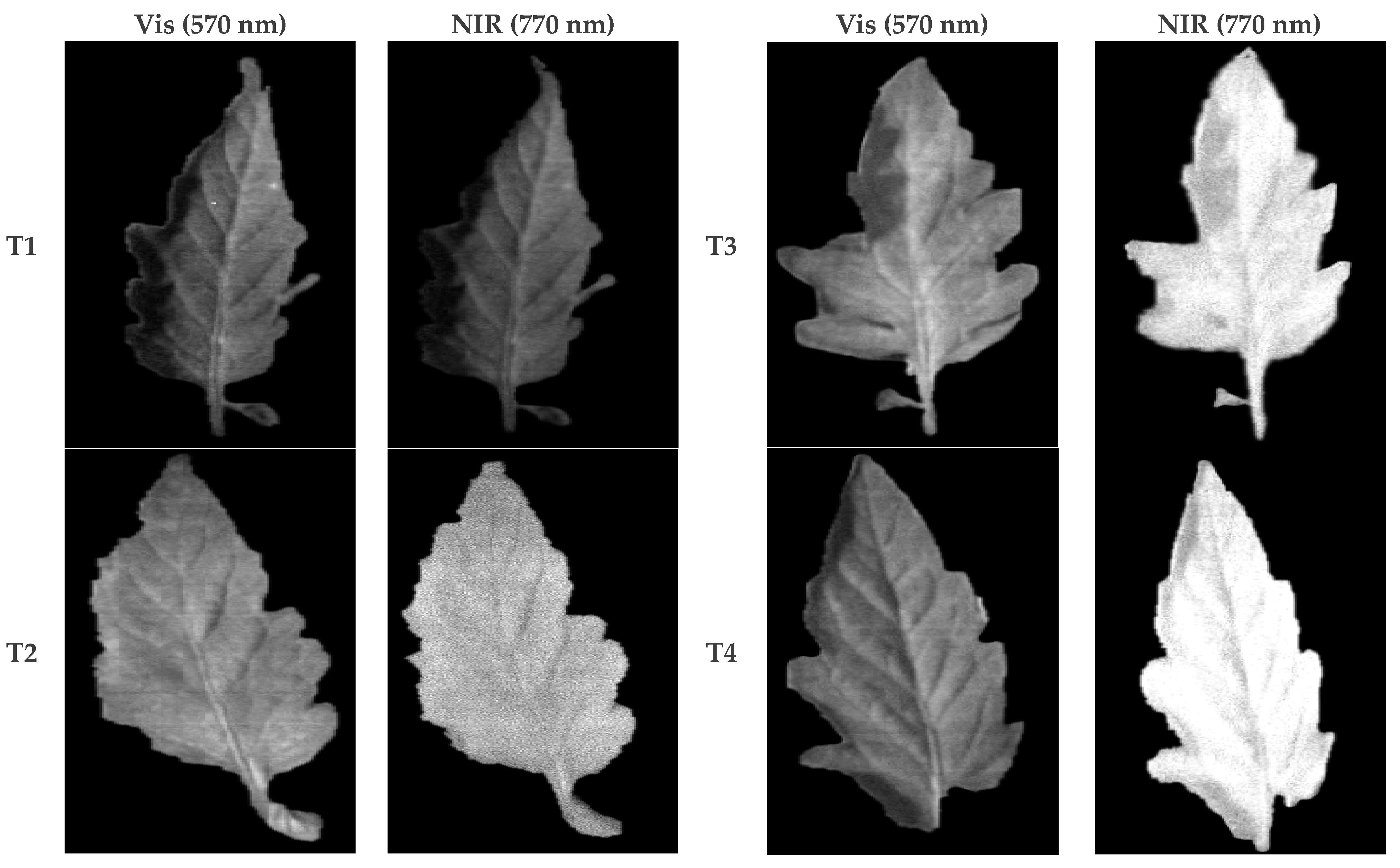
2.2. Hyperspectral Imaging and Spectral Information Extraction

The hardware system used to obtain the hyperspectral images was composed of the following components: (1) a hyperspectral camera in the Vis-NIR range (Physics Noor Co., Fanavaran, Kashan, Iran); (2) a laptop running Microsoft Windows 10 with an Intel Core i7 processor at 3.00 GHz and 16 GB of RAM; (3) a pair of tungsten halogen lights; and (4) a lighting chamber to reduce the influence of ambient light. Some examples of the obtained hyperspectral images at wavelengths between 400 and 1100 nm are presented in Figure 2 for the four classes of interest (T1, T2, T3, and T4). The number of captured spectral bands per image was 327, with an average spectral resolution of 2.5 nm.

A pre-processing step was used to reduce the impact of noise in the original spectral data. Hence, reflection spectral data were converted into absorption data using the inverse log relationship:

Absorption spectra = log(1/(Reflectance spectra))

(1)

A standard variate with a wavelet modification was used to correct the light scattering. Smoothing was enhanced with the Savitzki–Golay filter [26]. This method was done using ParLeS v3.1 software (Raphael Viscarra Rossel, Perth, Australia), a well-known chemical software for multivariate modeling.

Finally, from each hyperspectral image of the leaves, several patches of pixels are extracted (around 4 patches per image), obtaining tuples of 327 values. Each tuple represents the Vis-NIR spectrum at a given point on the leaves, and they are the input to the nitrogen content classifiers. In total, we have 1625 hyperspectral samples of the tomato leaves, of which 372 were selected for class T1, 402 for class T2, 462 for class T3, and 389 for class T4. Figure 3 shows some samples of these tuples that represent the spectra of the leaves for the four defined classes.

2.3. CNN for Nitrogen Content Estimation

Convolutional neural networks (CNNs) have become very popular for extracting spectral-spatial information in deep learning [10]. In this regard, we have specifically focused on CNNs for hyperspectral image estimation of nitrogen overdose in tomato leaves. The proposed CNN classifier was introduced by Benmouna et al. [27], which is used as a basis to investigate the performance of the proposed attention mechanism for predicting nitrogen content in tomato leaves. The input to the classifier is the spectral information of the tomato leaves after the execution of the pre-processing procedure described in the previous section (a 327-valued tuple). Additionally, the output is the treatment classes T1, T2, T3, and T4, corresponding to the number of days after nitrogen overapplication, from 0 to 3.

The sequential building components of the CNN structure are as follows: six convolutional layers, four max-pooling layers, a flattening layer, and a dense layer. The ReLU (rectified linear unit) activation function was used in all convolutional layers, while the soft-max activation function was used in the dense layer to obtain the output. More specifically, the CNN model is described in detail in

Table 1. Proposed convolutional neural network (CNN) structure for the prediction of nitrogen overdose in tomato leaves. The total number of trainable parameters is 1,036,356.

Layer (Type)	Filter Size	Number of Filters	Output Shape	Parameters
Conv1D_1	13 × 1	64	(316, 64)	832
Max_pooling1d_1			(158, 64)	0
Conv1D_2	5 × 64	128	(154, 128)	41,088
Conv1D_3	5 × 64	128	(150, 128)	82,048
Max_pooling1D_2			(75, 128)	0
Conv1D_4	5 × 128	256	(71, 256)	164,096
Max_pooling1d_3			(35, 256)	0
Conv1D_5	5 × 256	256	(31, 256)	327,936
Max_pooling1d_4			(15, 256)	0
Conv1D_5	3 × 256	512	(13, 512)	393,728
Flatten			(6656)	0
Dense			(4)	26,628

. The structure of this network is graphically shown in Figure 4.

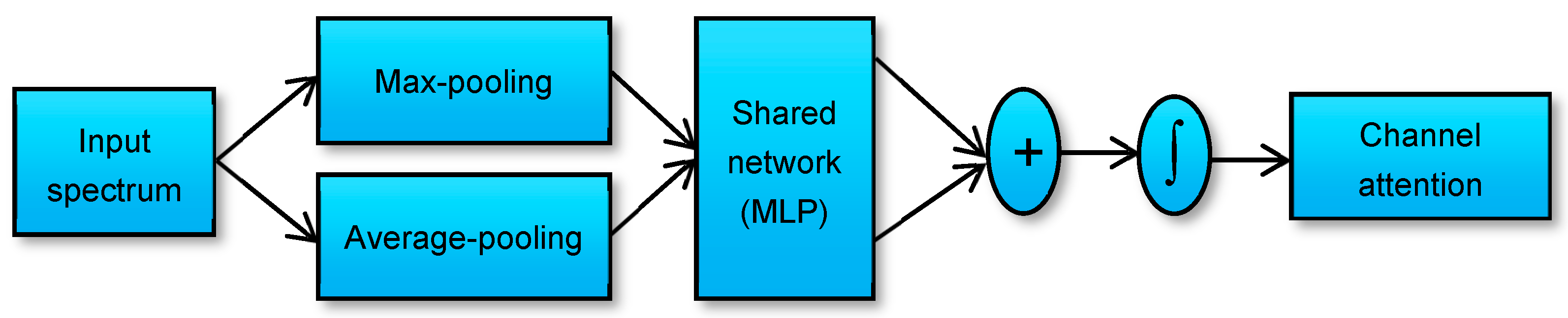
2.4. Attention-Based CNN for Nitrogen Estimation

Attention has become an increasingly important concept in the field of deep learning [28]. It takes its inspiration from the biological systems of humans, which prefer to focus on salient details while processing a lot of information. The attention mechanisms were first created in 2014 for applications involving natural language processing, and since then, they have been extensively utilized for a variety of purposes, particularly for computer vision tasks [29]. The attention mechanism’s basic concept is to allow the model to adaptively assign different weights to different types of information according to the task. Attention mechanism techniques can be divided into four categories. The first attention mechanism approach was proposed for natural language processing. This approach automatically selects every useful word or sub-sequence in a source language for translation into a target language using an encoder in a sequence-to-sequence prediction model [30]. Visual attention mechanisms are widely applied in computer vision tasks, including medical image segmentation [31], neural classification [32], and video processing [33].

The self-attention mechanism calculates location as the weighted sum of each feature at a position. Self-attention techniques are divided into spatial and channel attention approaches. The information interconnections between channels are not taken into account by spatial attention. Spatial attention, on the other hand, considers each channel’s output features to the same degree. In a similar way, channel attention ignores information exchanges in the spatial dimension [30].

Spatial and channel attention mechanisms have been shown to significantly improve the performance of deep CNNs. For example, Wang et al. [34] proposed an effective channel attention (ECA), which provided significant performance benefits through 1D CNN by adding only a few parameters. The experimental findings suggested that the ECA module is more effective for object detection and instance segmentation. From another perspective, Woo et al. [35] developed a convolutional block attention module (CBAM)-based channel and spatial attention modules for image classification and object detection. The effectiveness of CBAM was validated through extensive experiments on multiple image datasets (Net-1K, MS COCO, and VOC 2007). The experimental results showed that CBAM was able to very accurately classify the images.

Therefore, we propose in this study a spectral channel attention mechanism, a new approach introduced by Woo et al. [35], to improve the representation capacity of the CNN classifier. The proposed attention mechanism was designed and adjusted for the purpose of improving the predictive performance of the proposed CNN for the estimation of nitrogen overdose in tomato leaves. The channel attention module consists of max-polling and average-polling operations with a shared network. The shared network consists of a single hidden layer of a multi-layer perceptron (MLP). Figure 5 illustrates the overview of the proposed channel attention module. The information of the input spectral feature map, F, is first aggregated by applying both average-pooling and max-pooling operations, which generate two distinct spectral descriptors, F^C_average and F^C_maxpool, which refer to average-pooled and maximum-pooled features, respectively. Then, both descriptors are subsequently transmitted to a shared network to produce a 1D channel attention map, M_ca ∈ R^C×1. To keep the parameter overhead to a minimum, the hidden activation size is set to R ^C/r×1, where r represents the reduction ratio. After that, element-wise summing is used to combine the output feature vectors after the shared network has been applied to each descriptor. The channel attention can be denoted using the following equation:

M_c(F) = σ(W₀ (W₁ (F^C_average)) + W₀ (W₁ (F^C_maxpool)))

(2)

where σ represents the sigmoid function, W₀ ∈ R ^{C/C *r}, and W₁ ∈ R ^{C* C/r}.

It should be noted that the ReLU activation function is followed by W₀, and the MLP weights (W₀ and W₁) are shared for both descriptors.

Table 2. Proposed convolutional neural network (CNN) structure with an attention mechanism for the prediction of nitrogen overdose in tomato leaves.

Layer (Type)	Filter Size	Number of Filters	Output Shape	Parameters
Channel_attention			(327, 1)	0
Conv1D_1	13 × 1	64	(316, 64)	832
Max_pooling1d_1			(158, 64)	0
Conv1D_2	5 × 64	128	(154, 128)	41,088
Conv1D_3	5 × 64	128	(150, 128)	82,048
Max_pooling1D_2			(75, 128)	0
Conv1D_4	5 × 128	256	(71, 256)	164,096
Max_pooling1d_3			(35, 256)	0
Conv1D_5	5 × 256	256	(31, 256)	327,936
Max_pooling1d_4			(15, 256)	0
Conv1D_5	3 × 256	512	(13, 512)	393,728
Flatten			(6656)	0
Dense			(4)	26,628

depicts the proposed structure of the CNN with an attention mechanism, for the prediction of nitrogen overdose in tomato leaves.

3. Results

In this section, we describe the experimental results obtained with the two proposed CNN models (with/without attention mechanism) on the dataset of tomato leaf images. The tomato leaf samples (1625 tuples) were randomly divided into a training set and a test set. For this purpose, 1137 samples (70%) were randomly selected for training, while the remaining 488 samples (30%) were selected for testing. The categorical cross-entropy loss function (the cross-entropy between the labels and predictions) was used to measure the performance of each CNN model, and the Adam optimizer with a learning rate of 0.0001 was used to update the weights of each of the CNN models. The maximum number of epochs was 100, and the batch size was 8. Both CNN models were programmed and run on the JupyterLab interface using the Python programming language (version 3.9.0) and a laptop equipped with an Intel Core i7 processor clocked at 3.00 GHz and 16 GB of RAM.

The training and testing process was repeated three times for each run, using three different random seeds (denoted by 0, 1, and 2) to divide the dataset into training and test sets. At each repetition, a confusion matrix was obtained, and all these confusion matrices were added together to give the overall confusion matrix. The results of each repetition and the average of the three are presented. Various performance metrics extracted from the overall confusion matrix were used in this study, including the correct classification rate (CCR), recall, precision, specificity, FP-rate, and F-score. In addition, the area under the receiver operating characteristic (AUC) curve is also presented for each class.

The first experiment developed consists of obtaining the optimal values of the learning rate and batch size hyperparameters. Then, with the optimal values obtained, the accuracy of the CNN is analyzed both with and without the attention mechanism. Then, another important factor is analyzed, which is the number of examples available for training. We study how both CNN models behave as the number of training examples is reduced. Finally, a comparison of the proposed CNN with two classical neural networks, AlexNet and VGGNet, including and not including the attention mechanism, has been carried out.

3.1. Determining the Optimal Learning Rate and Batch Size for the CNN

First, we investigate the impact of two important hyperparameters of the training process on the effectiveness of the proposed CNN with attention: the learning rate and the batch size. For this purpose, a comparative assessment was conducted in terms of the CCR to determine the optimal value of both hyperparameters. To evaluate their effect on the efficiency of the classifier, we trained the classifier three times using three different random-number seeds, changing the values of the parameters. Specifically, to determine the optimal batch size, we trained the model with four different batch sizes (1, 4, 8, and 16) over 100 training epochs, using a fixed learning rate of 0.0001.

Then, the batch size that achieved the best CCR was considered the optimal one. Similarly, to determine the optimal learning rate, we trained the model with three different learning rates (0.001, 0.0001, and 0.00001) over 100 training epochs, using the optimal batch size obtained in the previous step.

Table 3. Overall correct classification rate (CCR) of the proposed attention mechanism-based CNN obtained with four different batch sizes (1, 4, 8, and 16), using a training set size of 70%, and a fixed learning rate of 0.0001.

Model	Training Set Size	Learning Rate	Epochs	Batch Size	Random Seed	CCR (%)	Overall CCR (%)
CNN with attention mechanism	70%	0.0001	100	1	0	96.10	94.32
					1	92.21
					2	94.67
				4	0	96.51	96.64
					1	95.69
					2	97.74
				8	0	96.51	97.33
					1	97.33
					2	98.15
				16	0	95.08	96.31
					1	96.72
					2	97.13

shows the overall CCR of the classifier obtained with four different batch sizes (1, 4, 8, and 16), using a training set size of 70% of the dataset, and a fixed learning rate of 0.0001.

According to these results, the best classification was achieved with a batch size of 8, reaching a CCR of 97.33%. It is observed that, starting from a value of 94.32% for the batch size, the CCR increases progressively as the batch size used increases. However, after the optimal size of 8, the CCR decreases for size 16. The results for all three seeds indicate fairly stable results for each size. Consequently, the optimum batch size of the proposed method was set at 8. Regarding the study of the learning rate,

Table 4. Overall correct classification rate (CCR) of the proposed attention mechanism-based CNN obtained with three different learning rates (0.001, 0.0001, and 0.00001), using a batch size of 8 and a training set size of 70%.

Model	Training Set Size	Batch Size	Epochs	Learning Rate	Random State	CCR (%)	Overall CCR (%)
CNN with attention mechanism	70%	8	100	0.001	0	91.39	92.89
					1	91.39
					2	95.90
				0.0001	0	96.51	97.33
					1	97.33
					2	98.15
				0.00001	0	95.90	96.10
					1	95.90
					2	96.51

contains the overall CCR of the proposed CNN with attention obtained with three different learning rates (0.001, 0.0001, and 0.00001), using a batch size of 8 and a training set size of 70%. Figure 6 shows the accuracies of these configurations over the 100 training epochs for the three repetitions of each case.

The results obtained indicate that the best classification was achieved with a learning rate of 0.0001, reaching a CCR of 97.33%. The difference with respect to the learning rate of 0.001 is significant, achieving only a 92.89% CCR. As shown in Figure 6a, this can be due to the great instability of the training process for the 0.001 value. However, for the smaller learning rates of 0.0001 and 0.00001, the process reaches convergence at about 80 epochs. In the case of 0.00001, the three random repetitions obtain very close results, although the average CCR is slightly worse, at 96.10%. In addition, we see a correlation between batch size and learning rate: when the learning rate is low, the large batch performs better than when the learning rate is high. It can be concluded that the performance of the proposed attention mechanism is significantly influenced by the learning rate and the batch size. Therefore, the leaning rate is fixed at 0.0001 for the batch size of 8.

3.2. Nitrogen Estimation Using CNN without Attention

As previously described, after determining the optimal values of the hyperparameters, the overall CCR of the CNN without attention was obtained from three different repetitions using different random seeds (0, 1, and 2), where a batch size of 8 and a learning rate of 0.0001 were used to train the model in each experiment. The results obtained are presented in

Table 5. Overall correct classification rate (CCR) of the CNN model without attention obtained for three different repetitions.

Model	Training Set Size	Batch Size	Learning Rate	Epochs	Random Seed	Training Time (Min:Sec)	CCR (%)	Overall CCR (%)
CNN		8	0.0001		0	13:19	94.46	94.94
	70%			100	1	11:57	94.87
					2	15:35	95.49

.

As a result, the CCR of the CNN classifier without attention was 94.94%, indicating that this method is able to achieve accurate predictions for the nitrogen content in tomato leaves. These results are very stable, with only a 1% difference between the best and the worst repetitions.

Table 6. Performance evaluation of the CNN without attention, including the overall confusion matrix, the overall classification error per class, the overall area under the ROC curve (AUC), and the overall correct classification rate (CCR). Columns: expected class; rows: obtained class.

Class	T1	T2	T3	T4	Overall Classification Error per Class (%)	Overall AUC	Overall CCR (%)
T1	295	2	34	3	3.89	0.93	94.94
T2	4	357	4	0	0.73	0.98
T3	13	6	390	0	1.54	0.95
T4	3	0	0	353	0.28	0.99

presents the overall confusion matrix of the CNN classifier without attention, obtained from the sum of the three different executions.

The obtained confusion matrix reveals that only 69 of the 1464 samples were misclassified in a class other than the expected class. Most of the errors are caused by confusions between classes T1 and T3, and T4 is the class that is classified with the best accuracy, only with a 0.28% classification error.

Table 7. Performance evaluation of the CNN without attention for classes T1, T2, T3, and T4 using different criteria.

Class	Recall	Accuracy	Specificity	FP-Rate	Precision	F-Score
T1	88.32	95.96	98.23	1.76	93.65	90.90
T2	97.80	98.90	99.27	0.72	97.80	97.80
T3	95.35	96.10	96.39	3.60	91.12	93.18
T4	99.15	99.59	99.72	0.27	99.15	99.15

evaluates the performance of the CNN classifier without attention using the six criteria mentioned above. According to the results, the highest recall (99.15%) is found in class T4, which means that most samples were correctly classified in this class. Class T3 has the lowest specificity value (96.39%), which indicates that this class contains many samples that are misclassified into other classes. The best precision is found in class T4, meaning that many leaf samples of this class are accurately classified; thus, the low precision obtained for class T3 (91.12%) means that many leaf samples of this class are not accurately identified.

3.3. Nitrogen Estimation Using CNN with Attention Mechanism

The overall CCR of the proposed CNN with an attention mechanism is shown in

Table 8. Overall correct classification rate (CCR) of the proposed attention mechanism-based CNN obtained from three different repetitions.

Model	Training Set Size	Batch Size	Learning Rate	Epochs	Random Seed	Training Time (Min:Sec)	CCR (%)	Overall CCR (%)
CNN with attention mechanism		8	0.0001		0	10:57	96.51	97.33
	70%			100	1	11:39	97.33
					2	12:12	98.15

, again obtained from three different repetitions, a batch size of 8, and a learning rate of 0.0001.

The obtained results demonstrate that the effectiveness of this classifier achieved a higher identification accuracy, reaching 97.33%, which is 2.39% better than that obtained by the CNN without attention. Moreover, the training time is not affected by the introduction of the attention network. Instead, the proposed mechanism is able to improve the convergence of the method, thus reducing slightly the total training time.

Table 9. Performance evaluation of the CNN with attention, including the overall confusion matrix, the overall classification error per class, the overall area under the ROC curve (AUC), and the overall correct classification rate (CCR). Columns: expected class; rows: obtained class.

Class	T1	T2	T3	T4	Overall Classification Error per Class (%)	Overall AUC	Overall CCR (%)
T1	313	1	14	1	1.62	0.97	97.33
T2	2	364	6	0	0.71	0.98
T3	8	6	402	0	1.12	0.97
T4	1	0	0	346	0.096	1.00

presents the overall confusion matrix of the attention mechanism-based CNN classifier, summing up the three repetitions. As can be observed, there were only 13 incorrectly classified samples out of a total of 1464. As in the CNN without attention, class T1 has the highest overall classification error, but in this case, it is only 1.62%.

The performance evaluation of the proposed attention mechanism for classes T1, T2, T3, and T4 using the six defined criteria is contained in

Table 10. Performance evaluation of CNN with attention mechanism for classes T1, T2, T3, and T4 using different criteria.

Class	Recall	Accuracy	Specificity	FP-Rate	Precision	F-Score
T1	95.13	98.15	99.03	0.96	96.60	95.86
T2	97.84	98.97	99.35	0.64	98.11	97.98
T3	96.63	97.67	98.09	1.90	95.26	95.94
T4	99.71	99.86	99.91	0.089	99.71	99.71

. As shown, the high recall (99.71%) obtained for class T4 means that many leaf samples are correctly classified in this class; thus, the low recall obtained for class T1 (95.13%) means that many leaf samples were misclassified in different classes. Compared to the other classes, class T2 has a recall rate of 97.84%, demonstrating that very few samples from other classes were misclassified as belonging to this class. The greatest accuracy value (99.86%) in class T4 suggests that many samples are successfully classified in this class. Class T4 has the highest specificity (99.91%), indicating that very few samples in that class are misclassified in comparison to other classes. Class T3 has the lowest specificity (98.09%); therefore, it contains many samples that are misclassified into other classes. Class T2 has a specificity of 99.35%, which is better than that obtained by classes T1 and T3, demonstrating that a very few samples in class T2 are misclassified in comparison to these classes. The best precision is found in classes T2 and T4, which indicates that many leaf samples in these classes are accurately classified.

These results demonstrate that the proposed attention mechanism-based CNN classifier is able to estimate the excessive use of nitrogen fertilizer in tomatoes early, even after the first 24 h. This allows farmers to take immediate corrective measures to avoid the risk of crop failure. If we consider a binary classification of normal/excessive nitrogen, then the classification accuracy would rise to 98.16%, while it would be 95.97% without attention.

3.4. Comparison of the CNN with/without Attention with Respect to the Training Set Size

Another important aspect of deep neural networks that is interesting to analyze is their ability to produce good results with a larger or smaller number of samples. This makes it possible to observe whether the system is able to produce good results in cases where less information is available. Thus, in this section, we study the impact of the size of the training data on the two proposed CNN classifiers, with and without attention mechanisms. For this purpose, the same size of the test set (30%) was used, while the classifiers were trained with three different training set sizes (30%, 50%, and 70% of the total dataset), which were randomly selected in three repetitions with three random seeds. This corresponds to 487 samples (30%), 812 samples (50%), and 1137 samples (70%) for training. In this case, the optimal values found for the batch size of 8 and learning rate of 0.0001 were used.

Table 11. Overall CCR of the CNN classifier with attention mechanism obtained with three different training set sizes (30%, 50%, and 70%) over 100 training epochs, using a batch size of 8, a learning rate of 0.0001, and three random repetitions.

Model	Learning Rate	Batch Size	Epochs	Training Set Size	Random State	CCR (%)	Overall CCR (%)
CNN with attention mechanism	0.0001	8	100	30%	0	91.18	92.61
					1	91.18
					2	95.49
				50%	0	92.62	95.14
					1	95.49
					2	97.33
				70%	0	96.51	97.33
					1	97.33
					2	98.15

and

Table 12. Overall CCR of the CNN classifier without attention mechanism obtained with three different training set sizes (30%, 50%, and 70%) over 100 training epochs, using a batch size of 8, a learning rate of 0.0001, and three random repetitions.

Model	Learning Rate	Batch Size	Epochs	Training Set Size	Random State	CCR (%)	Overall CCR (%)
CNN without attention	0.0001	8	100	30%	0	92.00	93.16
					1	92.82
					2	94.67
				50%	0	91.93	93.48
					1	93.23
					2	95.28
				70%	0	94.46	94.94
					1	94.94
					2	94.87

present the overall CCR of the CNN classifiers with and without attention, respectively, for these configurations of the training process. The evolution of the accuracy of these CNNs during the training process is shown in Figure 7 and Figure 8.

The results prove again that the proposed attention mechanism is able to improve the accuracy of the underlaying CNN classifier. For a training size of 50%, the attention network introduces an average improvement of 1.66% in the CCR, and 2.39% for 70% training samples. However, when only 30% of training samples are used, the effect of the attention mechanism is a slight decrease in the CCR of 0.55%. According to these results, it can be concluded that a large training set provides improved performance compared to a small training set. The attention mechanism is more effective as more information becomes available, since it allows a better selection of the information of interest.

3.5. Comparison of the Proposed Model with AlexNet and VGGNet

The last set of experiments consists of a comparison of the proposed model with other alternative classifiers based on convolutional neural networks. For this purpose, two classic and well-known architectures have been used: AlexNet [36] and VGGNet (VGG16) [37]. In fact, the ultimate goal is not to compare the results of these models with the proposed CNN, but to evaluate the positive effect of the proposed attention mechanism on these existing models. Figure 9 shows the structure of the layers of these networks, whose exact definition can be found in the referenced papers.

Both networks were trained in similar conditions to the proposed CNN, that is, training for 100 epochs, with a batch size of 8, a learning rate of 0.0001, and 70% training samples. The process was executed for AlexNet and VGGNet, both with and without the attention mechanism, and each test was repeated with the same three random seeds as in the previous sections. The results obtained are shown in

Table 13. Overall correct classification rate (CCR) and training time obtained for the two architectures used for comparison, AlexNet and VGGNet, with and without the proposed attention mechanism, obtained from three different repetitions.

Model	Training Set Size	Batch Size	Learning Rate	Epochs	Random Seed	Training Time (Hr:Min:Sec)	CCR (%)	Overall CCR (%)
AlexNet		8	0.0001		0	1:34:36	81.56	81.00
	70%			100	1	1:34:46	78.68
					2	1:37:26	82.78
AlexNet with attention	70%	8	0.0001	100	0	1:23:20	85.05
					1	1:23:04	86.06	86.20
					2	1:28:20	87.50
VGGNet	70%	8	0.0001	100	0	1:22:06	92.82
					1	1:26:28	97.13	94.53
					2	1:28:02	93.64
VGGNet with attention	70%	8	0.0001	100	0	1:15:01	97.33
					1	1:15:25	96.92	97.54
					2	1:15:47	98.36

.

Again, the benefit of the attention mechanism can be seen very clearly, achieving an improvement in the overall CCR of 5% for AlexNet and 3% for VGGNet. This increase occurred with all seeds, although only in the case of seed 1 with VGGNet was there a small reduction (from 97.13% to 96.92%). The beneficial effect on execution time is also observed, with a slight reduction in training times when the attention mechanism is introduced by improving the convergence of the network. On the other hand, comparing the results obtained with those of the proposed CNN, the accuracy is very similar for the VGGNet model, while the AlexNet results are very poor, with a CCR of around 86%. In fact, VGGNet with attention mechanism achieves a CCR of 97.54%, slightly above the proposed CNN with attention of 97.33%. However, it is important to consider that the execution time of VGGNet is about 7 times slower than the proposed CNN (1 h and 15 min of the former versus about 11 min of the latter). This is due to the larger number of trainable parameters in the two classical models. While the proposed CNN method has about 1 million parameters, AlexNet has more than 54 million, and VGGNet has more than 30 million.

4. Discussion

The experimental findings of this study demonstrate that hyperspectral imaging is an effective technique for identifying excessive amounts of nitrogen in tomato leaves at an early stage. Both CNN classifiers (with/without attention mechanism) achieved an average classification accuracy for the four classes (T1, T2, T3, and T4) above 94%. However, there is still potential for development, and further study should be conducted before using these methods in real-world outdoor and distant sensing applications. The key findings of this research are as follows:

• In the present study, two classification methods were compared using CNNs with and without attention mechanisms. The same CNN architecture and the same CNN model parameter configuration were used in both classifiers. Both CNN classifiers were trained three times using three different random seeds, with a training set size of 70%, a batch size of 8, and a learning rate of 0.0001 used to train the models in each experiment. To evaluate the effectiveness of the proposed attention mechanism-based CNN method, the proposed CNN model was trained with four different batch sizes (1, 4, 8, and 16) and three learning rates (0.001, 0.0001, and 0.00001). To investigate the effect of the training data size on the efficiency of the proposed method, the CNN model was trained with three different training set sizes (30%, 50%, and 70%).
• The experimental results showed that the proposed CNN with attention mechanism performed better when using a training set size of 70% and when using a batch size of 8 with a learning rate of 0.0001, achieving an overall CCR of 97.33% over 100 training epochs. These results indicate that the use of large training data with a small batch size and a low training rate can improve the proposed attention mechanism’s ability to provide more accurate and reliable results. Larger batch sizes negatively affect accuracy, while smaller learning rates make the training process convergence much slower. The alternative CNN classifier performed worse than the CNN with an attention mechanism, achieving an overall CCR of 94.94%, which is 2.39% lower than that obtained by the CNN with an attention mechanism.
• The obtained results suggest that the proposed attention mechanism-based CNN is a feasible method for detecting the amount of nitrogen overdose even after 24 h. This enables the farmers to take immediate corrective measures to prevent the risk of crop failure. Additionally, the nitrogen content estimation was very accurate for the first day (class T2), with only a 0.71% error for the CNN classifier with an attention mechanism. Since the fertilizer is mixed with irrigation water, the plants absorb it quickly, enabling early detection on the leaves. The precision of classes T2 and T4 is better than that of classes T1 and T3, indicating that most samples in those classes are correctly classified. These results are very promising for the practical feasibility of the proposed method. The error is consistently higher for class T1 in all the models, indicating some possible problem in the sampling and capture process. To increase precision and make the technique more robust to individual mistakes, a real use of the system should involve testing different leaves for each plant.
• Regarding the evaluation of the time required for the execution of the training process, the total time required for the execution of the training process of the attention mechanism-based CNN model was about 33 min and 45 s, while the total time required for the execution of the training process of the CNN model without attention was about 40 min and 51 s. It can be deduced that the proposed attention method is not only able to improve the accuracy of the system, but it also reduces the training time by improving the convergence of the network.
• The comparison of the proposed method with two classic neural networks, AlexNet and VGGNet, has clearly proven the positive effect of introducing the attention mechanism as the first step of the network. The improvement of the attention layers in both models varies from 5% for AlexNet to 3% for VGGNet, compared to 2.4% for the proposed CNN. Obviously, as the CCR of the model without attention is higher, the ability of the attention mechanism to improve this accuracy is smaller. VGGNet with attention achieves an excellent CCR of 97.54%, slightly higher than the proposed CNN with attention. However, the VGGNet method is more computationally expensive, with 30 times more training parameters. This translated into a slower training process, which required more than one hour for each execution. It can be concluded that the proposed CNN model is the most cost-effective from the point of view of the accuracy obtained.
• Several studies have been conducted to estimate the nitrogen content in the leaves of plants using hyperspectral images, most of them dealing with regression issues. For example, Du et al. [38] applied support vector machine (SVM) regression on rice leaves, obtaining a coefficient of determination (R²) of 0.75. Liang et al. [39] applied random forest regression (RFR) and least squares support vector regression (LS-SVR) models on wheat leaves with an R² of 0.75. In another study, Fan et al. [40] used partial least squares (PLS) regression on corn leaves, achieving an R² of 0.77. In some recent studies, Yang et al. [41] proposed three machine learning techniques, gradient boosting decision tree (GBDT), partial least squares regression (PLS), and support vector regression (SVR), on wheat leaves; the best model was GBDT with calibration and validation R² of 0.975 and 0.861, respectively. Pourdarbani et al. [42] developed a 1D-CNN regression model to classify different nitrogen fertilizer treatments (30%, 60%, and 90% excess) in cucumber leaves. The spectral information of the cucumber leaves of four classes (control, 30%, 60%, and 90%) was studied. The results indicated that the classes 30%, 60%, and 90% had coefficients of determination of 0.962, 0.968, and 0.967, respectively. Hyperspectral imaging techniques were used in each of these studies to estimate the amount of nitrogen in plant leaves. In general, it can be seen that the most advanced techniques based on deep learning and convolutional neural networks are able to obtain the best results. However, the aim of this study is not related to the direct estimation of the amount of nitrogen in plants but to detect the misapplication of nitrogen fertilizers in plants. We are therefore dealing with a problem of classification of nitrogen treatments rather than a case of regression. Although these studies were selected among the most comparable to our case in the field of the estimation of the nitrogen content in plant leaves, this comparison must be viewed in context since they used different types of plants, capture tools, datasets, and classification models.
• Although the results obtained are very promising, two main limitations of the methodology proposed in this research can be highlighted. The first limitation is that the imaging is performed under laboratory conditions. This means that the study was conducted in a controlled environment, which may not fully represent outdoor conditions. It is important to validate the findings of the study by conducting similar experiments in more realistic settings, such as actual agricultural fields or greenhouses, to assess the effectiveness of the proposed approach in practical scenarios. The second limitation is the pixel-by-pixel processing done on the images. This implies that the analysis and processing of the images are performed on individual pixels rather than considering the entire image as a whole. While this approach may have its advantages, such as fine-grained analysis at the pixel level, it may not capture the broader context and spatial relationships between different regions of the image. Future research could explore methodologies that take into account the global features and relationships within the images to improve the accuracy and efficiency of the analysis.

5. Conclusions

Nitrogen is a crucial macronutrient for crop growth and yield, but excessive application can affect flavor and quality. This study proposed an approach using CNN with attention to classify leaf nitrogen treatments in tomatoes of the Royal variety. Hyperspectral imaging in the 400–1100 nm range captured spectral data for normal treatment and 30% overdose after 1, 2, and 3 days. The proposed attention mechanism used extracted features, and it was compared to a CNN without attention.

The experimental results showed that the proposed CNN with attention performed better, achieving a correct classification rate (CCR) of 97.33% over 100 training epochs, which is 2.39% higher than without attention. Moreover, the experiments also prove the positive effect of the proposed mechanism in two existing CNN models, AlexNet and VGGNet. The obtained results indicate that the use of a large training dataset (70% of the total dataset) with a small batch size (8) and a low training rate (0.0001) can improve the ability of the proposed attention mechanism to provide more accurate and reliable results. For smaller training datasets of 50% of the total, the effectiveness of the attention method may be lower. On the other hand, the computational efficiency of the proposed attention method is very high, since it is able to improve the convergence of the training process.

These results prove that the proposed method is a feasible tool for early estimation of nitrogen overdose in tomato leaves. These results can be applied to the development of new technologies for remote sensing-based detection of fertilizer overdose. However, the main limitation of the study is that the imaging was performed under laboratory conditions. In addition, processing is done pixel by pixel, not by whole images. Future research should address new issues for this purpose; for example, it will be interesting to study the effectiveness of the proposed approach for other crops. Another potential area of future study is the development of a novel CNN architecture with an attention mechanism that would be able to learn spatial and spectral feature information from hyperspectral images to jointly detect abnormal (pale and twisted) leaves and excess nitrogen.

References

1. Brentrup, F.; Pallière, C. Nitrogen Use Efficiency as an Agro-Environmental Indicator. In Proceedings of the OECD Workshop on Agrienvironmental Indicators, Leysin, Switzerland, 23–26 March 2010; pp. 23–26. [Google Scholar]
2. Warner, J.; Zhang, T.Q.; Hao, X. Effects of nitrogen fertilization on fruit yield and quality of processing tomatoes. Can. J. Plant Sci. 2004, 84, 865–871. [Google Scholar] [CrossRef]
3. Adhikary, S.; Biswas, B.; Naskar, M.K.; Mukherjee, B.; Singh, A.P.; Atta, K. Remote Sensing for Agricultural Applications. In Arid Environment; Elsevier: Amsterdam, The Netherlands, 2022. [Google Scholar]
4. Moghadam, P.; Ward, D.; Goan, E.; Jayawardena, S.; Sikka, P.; Hernandez, E. Plant Disease Detection Using Hyperspectral Imaging. In Proceedings of the 2017 International Conference on Digital Image Computing: Techniques and Applications (DICTA), Sydney, NSW, Australia, 29 November–1 December 2017; pp. 1–8. [Google Scholar]
5. Tao, H.; Feng, H.; Xu, L.; Miao, M.; Long, H.; Yue, J.; Li, Z.; Yang, G.; Yang, X.; Fan, L. Estimation of Crop Growth Parameters Using UAV-Based Hyperspectral Remote Sensing Data. Sensors 2020, 20, 1296. [Google Scholar] [CrossRef] [Green Version]
6. Park, E.; Kim, Y.-S.; Faqeerzada, M.A.; Kim, M.S.; Baek, I.; Cho, B.-K. Hyperspectral reflectance imaging for nondestructive evaluation of root rot in Korean ginseng (Panax ginseng Meyer). Front. Plant Sci. 2023, 14, 1109060. [Google Scholar] [CrossRef]
7. Nguyen, N.M.T.; Liou, N.-S. Ripeness Evaluation of Achacha Fruit Using Hyperspectral Image Data. Agriculture 2022, 12, 2145. [Google Scholar] [CrossRef]
8. Pourdarbani, R.; Sabzi, S.; Arribas, J.I. Nondestructive estimation of three apple fruit properties at various ripening levels with optimal Vis-NIR spectral wavelength regression data. Heliyon 2021, 7, e07942. [Google Scholar] [CrossRef]
9. Xuan, G.; Gao, C.; Shao, Y.; Wang, X.; Wang, Y.; Wang, K. Maturity determination at harvest and spatial assessment of moisture content in okra using Vis-NIR hyperspectral imaging. Postharvest Biol. Technol. 2021, 180, 111597. [Google Scholar] [CrossRef]
10. Sun, H.; Zheng, X.; Lu, X.; Wu, S. Spectral–Spatial Attention Network for Hyperspectral Image Classification. IEEE Trans. Geosci. Remote Sens. 2019, 58, 3232–3245. [Google Scholar] [CrossRef]
11. Mei, X.; Pan, E.; Ma, Y.; Dai, X.; Huang, J.; Fan, F.; Du, Q.; Zheng, H.; Ma, J. Spectral-Spatial Attention Networks for Hyperspectral Image Classification. Remote Sens. 2019, 11, 963. [Google Scholar] [CrossRef] [Green Version]
12. Nagasubramanian, K.; Jones, S.; Singh, A.K.; Sarkar, S.; Singh, A.; Ganapathysubramanian, B. Plant disease identification using explainable 3D deep learning on hyperspectral images. Plant Methods 2019, 15, 98. [Google Scholar] [CrossRef] [Green Version]
13. Zhu, Y.; Abdalla, A.; Tang, Z.; Cen, H. Improving rice nitrogen stress diagnosis by denoising strips in hyperspectral images via deep learning. Biosyst. Eng. 2022, 219, 165–176. [Google Scholar] [CrossRef]
14. Benmouna, B.; García-Mateos, G.; Sabzi, S.; Fernandez-Beltran, R.; Parras-Burgos, D.; Molina-Martínez, J.M. Convolutional Neural Networks for Estimating the Ripening State of Fuji Apples Using Visible and Near-Infrared Spectroscopy. Food Bioprocess Technol. 2023, 15, 2226–2236. [Google Scholar] [CrossRef]
15. Xiang, Y.; Chen, Q.; Su, Z.; Zhang, L.; Chen, Z.; Zhou, G.; Yao, Z.; Xuan, Q.; Cheng, Y. Deep Learning and Hyperspectral Images Based Tomato Soluble Solids Content and Firmness Estimation. Front. Plant Sci. 2022, 13, 860656. [Google Scholar] [CrossRef]
16. Jian, M.; Zhang, L.; Jin, H.; Li, X. 3DAGNet: 3D Deep Attention and Global Search Network for Pulmonary Nodule Detection. Electronics 2023, 12, 2333. [Google Scholar] [CrossRef]
17. Chuma, E.L.; Iano, Y. Human Movement Recognition System Using CW Doppler Radar Sensor with FFT and Convolutional Neural Network. In Proceedings of the 2020 IEEE MTT-S Latin America Microwave Conference (LAMC 2020), Cali, Colombia, 26–28 May 2021; pp. 1–4. [Google Scholar]
18. Baradaran, F.; Farzan, A.; Danishvar, S.; Sheykhivand, S. Customized 2D CNN Model for the Automatic Emotion Recognition Based on EEG Signals. Electronics 2023, 12, 2232. [Google Scholar] [CrossRef]
19. Liu, G.; Guo, J. Bidirectional LSTM with attention mechanism and convolutional layer for text classification. Neurocomputing 2019, 337, 325–338. [Google Scholar] [CrossRef]
20. Yang, J.; Sun, Y.; Liang, J.; Ren, B.; Lai, S.-H. Image captioning by incorporating affective concepts learned from both visual and textual components. Neurocomputing 2019, 328, 56–68. [Google Scholar] [CrossRef]
21. Jia, Y. Attention Mechanism in Machine Translation. J. Phys. Conf. Ser. 2019, 1314, 012186. [Google Scholar] [CrossRef]
22. Song, K.; Yao, T.; Ling, Q.; Mei, T. Boosting image sentiment analysis with visual attention. Neurocomputing 2018, 312, 218–228. [Google Scholar] [CrossRef]
23. Tian, H.; Wang, P.; Tansey, K.; Han, D.; Zhang, J.; Zhang, S.; Li, H. A deep learning framework under attention mechanism for wheat yield estimation using remotely sensed indices in the Guanzhong Plain, PR China. Int. J. Appl. Earth Obs. Geoinf. 2021, 102, 102375. [Google Scholar] [CrossRef]
24. Qian, X.; Zhang, C.; Chen, L.; Li, K. Deep Learning-Based Identification of Maize Leaf Diseases Is Improved by an Attention Mechanism: Self-Attention. Front. Plant Sci. 2022, 13, 864486. [Google Scholar] [CrossRef]
25. Wang, Y.; Tao, J.; Gao, H. Corn Disease Recognition Based on Attention Mechanism Network. Axioms 2022, 11, 480. [Google Scholar] [CrossRef]
26. Rossel, R.A.V. ParLeS: Software for chemometric analysis of spectroscopic data. Chemom. Intell. Lab. Syst. 2008, 90, 72–83. [Google Scholar] [CrossRef]
27. Benmouna, B.; Pourdarbani, R.; Sabzi, S.; Fernandez-Beltran, R.; García-Mateos, G.; Molina-Martínez, J.M. Comparison of Classic Classifiers, Metaheuristic Algorithms and Convolutional Neural Networks in Hyperspectral Classification of Nitrogen Treatment in Tomato Leaves. Remote Sens. 2022, 14, 6366. [Google Scholar] [CrossRef]
28. Niu, Z.; Zhong, G.; Yu, H. A review on the attention mechanism of deep learning. Neurocomputing 2021, 452, 48–62. [Google Scholar] [CrossRef]
29. Ghaffarian, S.; Valente, J.; van der Voort, M.; Tekinerdogan, B. Effect of Attention Mechanism in Deep Learning-Based Remote Sensing Image Processing: A Systematic Literature Review. Remote Sens. 2021, 13, 2965. [Google Scholar] [CrossRef]
30. Weng, W.; Zhu, X.; Jing, L.; Dong, M. Attention Mechanism Trained with Small Datasets for Biomedical Image Segmentation. Electronics 2023, 12, 682. [Google Scholar] [CrossRef]
31. Chen, J.; Lu, Y.; Yu, Q.; Luo, X.; Adeli, E.; Wang, Y.; Lu, L.; Yuille, A.L.; Zhou, Y. Transunet: Transformers Make Strong Encoders for Medical Image Segmentation. arXiv 2021, arXiv:2102.04306. [Google Scholar]
32. Wang, F.; Jiang, M.; Qian, C.; Yang, S.; Li, C.; Zhang, H.; Wang, X.; Tang, X. Residual Attention Network for Image Classification. In Proceedings of the IEEE Conference on Computer Vision and Pattern Recognition, Honolulu, HI, USA, 21–26 July 2017; pp. 3156–3164. [Google Scholar]
33. Ji, Z.; Xiong, K.; Pang, Y.; Li, X. Video Summarization with Attention-Based Encoder–Decoder Networks. IEEE Trans. Circuits Syst. Video Technol. 2019, 30, 1709–1717. [Google Scholar] [CrossRef] [Green Version]
34. Wang, Q.; Wu, B.; Zhu, P.; Li, P.; Zuo, W.; Hu, Q. ECA-Net: Efficient Channel Attention for Deep Convolutional Neural Networks. In Proceedings of the IEEE/CVF Conference on Computer Vision and Pattern Recognition, Seattle, WA, USA, 13–19 June 2020; pp. 11534–11542. [Google Scholar]
35. Woo, S.; Park, J.; Lee, J.Y.; Kweon, I.S. Cbam: Convolutional Block Attention Module. In Proceedings of the European Conference on Computer Vision (ECCV), Munich, Germany, 8–14 September 2018; pp. 3–19. [Google Scholar]
36. Krizhevsky, A.; Sutskever, I.; Hinton, G.E. Imagenet classification with deep convolutional neural networks. Commun. ACM 2017, 60, 84–90. [Google Scholar] [CrossRef] [Green Version]
37. Simonyan, K.; Zisserman, A. Very Deep Convolutional Networks for Large-Scale Image Recognition. arXiv 2014, arXiv:1409.1556. [Google Scholar]
38. Du, L.; Gong, W.; Shi, S.; Yang, J.; Sun, J.; Zhu, B.; Song, S. Estimation of Rice Leaf Nitrogen Contents Based on Hyperspectral LIDAR. Int. J. Appl. Earth Obs. Geoinf. 2016, 44, 136–143. [Google Scholar] [CrossRef]
39. Liang, L.; Di, L.; Huang, T.; Wang, J.; Lin, L.; Wang, L.; Yang, M. Estimation of Leaf Nitrogen Content in Wheat Using New Hyperspectral Indices and a Random Forest Regression Algorithm. Remote Sens. 2018, 10, 1940. [Google Scholar] [CrossRef] [Green Version]
40. Fan, L.; Zhao, J.; Xu, X.; Liang, D.; Yang, G.; Feng, H.; Wang, Y.; Chen, G.; Wei, P. Hyperspectral-Based Estimation of Leaf Nitrogen Content in Corn Using Optimal Selection of Multiple Spectral Variables. Sensors 2019, 19, 2898. [Google Scholar] [CrossRef] [Green Version]
41. Yang, B.; Ma, J.; Yao, X.; Cao, W.; Zhu, Y. Estimation of Leaf Nitrogen Content in Wheat Based on Fusion of Spectral Features and Deep Features from Near Infrared Hyperspectral Imagery. Sensors 2021, 21, 613. [Google Scholar] [CrossRef]
42. Pourdarbani, R.; Sabzi, S.; Rohban, M.H.; Hernández-Hernández, J.L.; Gallardo-Bernal, I.; Herrera-Miranda, I.; García-Mateos, G. One-Dimensional Convolutional Neural Networks for Hyperspectral Analysis of Nitrogen in Plant Leaves. Appl. Sci. 2021, 11, 11853. [Google Scholar] [CrossRef]
Figure 1. Main steps of the nitrogen treatment detection method in tomato leaves.
Electronics 12 02706 g001
Figure 2. Sample hyperspectral images of tomato leaves taken for the four treatments, T1, T2, T3, and T4, at two wavelengths in the visible (Vis) and near-infrared (NIR) spectra.
Electronics 12 02706 g002
Figure 3. Four samples of the obtained Vis-NIR spectra of the leaves taken from patches of the hyperspectral images, for the four treatments, T1, T2, T3, and T4.
Electronics 12 02706 g003
Figure 4. Architecture of the CNN models used for detecting the nitrogen treatment in tomato leaves. The types of layers are as follows: Input: input layer; Conv: 1D convolutional layer; Pool: max pooling layer; Flatten: flattening layer; FC: fully connected layer.
Electronics 12 02706 g004
Figure 5. Schematic diagram of the proposed channel attention module.
Electronics 12 02706 g005
Figure 6. Evolution of the accuracy (CCR) of the proposed CNN with attention mechanism with respect to the number of epochs, using a batch size of 8, a training set size of 70% of the total dataset, and three different learning rates: (a) 0.001; (b) 0.0001; (c) 0.00001. Each test is repeated with three random seeds.
Electronics 12 02706 g006aElectronics 12 02706 g006b
Figure 7. Evolution of the accuracy (CCR) of the proposed CNN with attention mechanism with respect to the number of epochs, using a batch size of 8, a learning rate of 0.0001, and three training set sizes: (a) 30%; (b) 50%; (c) 70%. Each test is repeated with three random seeds.
Electronics 12 02706 g007aElectronics 12 02706 g007b
Figure 8. Evolution of the accuracy (CCR) of the proposed CNN without attention mechanism with respect to the number of epochs, using a batch size of 8, a learning rate of 0.0001, and three training set sizes: (a) 30%; (b) 50%; (c) 70%. Each test is repeated with three random seeds.
Electronics 12 02706 g008aElectronics 12 02706 g008b
Figure 9. Architecture of the two classic CNN models used for comparison. (a) AlexNet [36], with 54,659,460 trainable parameters; (b) VGGNet (VGG16) [37], with 30,097,732 trainable parameters. The types of layers are as follows: Input: input layer; Conv: convolutional layer; Pool: max pooling layer; FC: fully connected layer; SoftMax: output soft-max layer.
Electronics 12 02706 g009