Nested Entity Recognition Fusing Span Relative Position and Region Information

Abstract

At present, span-based entity recognition methods are mainly used to accurately identify the span (entity) boundary for entity recognition, in which the relative position information of the span boundary and the information of words in the span region are routinely ignored. This information can be used to improve entity recognition performance. Therefore, a nested entity recognition model, which integrates the relative position information of the span and the region information within the span, is proposed. The span representation is first obtained with a triaffine attention. Then, the relative position of the span boundary and the word information in the span region, as well as the previous span representation, are fused to obtain a new label-level span representation with another triaffine attention. Finally, the span (entity) recognition task is carried out by a cooperative biaffine mechanism. Experiments were conducted on some public datasets, including ACE2004, ACE2005 and GENIA. The results show that the F1-scores achieved using the proposed method were 87.66%, 86.86% and 80.90% on ACE2004, ACE2005 and GENIA, respectively. These experiments show that the method achieved state-of-the-art (SOTA) results. Moreover, the proposed model has fewer parameters and needs fewer resources with a lower time complexity than the existing triaffine mechanism model.

1. Introduction

Named Entity Recognition (NER) is a basic natural language processing task used to extract meaningful entities from text. Traditional named entity recognition, also known as Flat Named Entity Recognition (Flat NER), is usually regarded as a sequence labeling problem [1], and has been well studied. However, nested entities with multi-granular semantic information are commonly available in text in all kinds of professional fields [2]. For nested entities, a single word may have multiple labels. Therefore, it is difficult to solve this problem based on sequence labeling frameworks.

In recent years, a variety of methods for nested entity recognition have been proposed, including sequential labeling methods that assign a label to each token from a predesigned labeling scheme [3,4,5,6], hypergraph-based modeling methods for nested named entity tasks [7,8,9], methods that label sequence to sequence (Seq2Seq) of all entities and output the starting position span length [10,11], and span-based methods for enumerating all possible entities in a sentence [12,13,14,15]. At present, the span-based method, which learns the possible representation of each span and then classifies it, is one of the most widely used methods for nested entity recognition [12,15,16,17,18,19]. Among span-based methods, those that leverage large-scale pre-training modules can achieve better results in nested entity recognition than other methods [18,19]. However, most of the works based on span focus on how to accurately identify the entity boundary. The relative position information of the span boundary and the information of words in the span region are routinely ignored.

In addition, there is an increasing demand for the accurate identification of nested entities in various domains, such as healthcare, finance, and law. In the healthcare domain, for example, accurate recognition of entities such as diseases, medications, and treatment plans is crucial for clinical decision-making and disease monitoring. In the finance domain, precise identification of entities such as companies, individuals, and transactions aids in risk assessment and market intelligence analysis. In the legal field, accurate identification of nested entities is of significant importance for case analysis and legal research.

Therefore, improving the accuracy and efficiency of named entity recognition has become a focus of research in both academia and industry. Addressing challenges in nested entity recognition, such as modeling nested entity structures, improving boundary identification accuracy, and leveraging span region information, is a pressing research problem that needs to be tackled. To improve the performance of span-based methods, Yuan et al. [14] proposed a triaffine transformation; that is, on the basis of a biaffine transformation, span internal information is represented in the third dimension. The internal region information of the span determined by the boundary is used as the span representation, as shown in Figure 1. The triaffine transformation is used to recognize the entity “the secretary of homeland security”. The left side of Figure 1 shows the span boundary represented by a biaffine transformation, and the entity can only be represented by the embedded mapping of “the” and “security”. The right side shows the third dimension of the triple affine. Based on the biaffine, the triaffine transformation further takes the fusion of the span boundary and internal information as the span representation (the entire embedded mapping, “the secretary of homeland security”, is used as the representation entity).

In this study, a method based on a dual-triaffine attention mechanism, which integrates the relative position of the span boundary and the region information, is proposed for nested entity recognition. In the first stage, interactive learning between the span and the boundary is achieved through triaffine attention, resulting in a high-dimensional span representation. In the second stage, the span representation, relative position information, and region information are fused, and a new label-level span representation is obtained using triaffine attention, which captures the high-order interaction between the span boundary and the fused information. Additionally, we consider the importance of entity boundary identification in nested entity recognition, and therefore, the collaborative prediction of span representation using both biaffine and triaffine attention is proposed. The main contributions of this paper are as follows: (1) the proposal of a triaffine attention mechanism that integrates the relative position of the span boundary and the information within the span region; (2) the introduction of a collaborative prediction model based on biaffine and triaffine attention, utilizing a similar residual connection for span category prediction. Experimental results obtained using the ACE2004, ACE2005, and GENIA datasets demonstrate the effectiveness of the proposed dual-triaffine attention and collaborative entity prediction using biaffine attention.

2. Related Work

2.1. Nested Named Entity Recognition

Nested Named Entity Recognition (Nested NER) methods can be categorized into four main types: (1) sequence labeling, (2) hypergraph-based, (3) sequence-to-sequence (Seq2Seq), and (4) span-based methods.

(1) Sequence labeling methods

Sequence-labeling-based methods usually view NER as a sequence labeling problem, assigning a tag to each token from a predesigned labeling scheme (such as BIO). Currently, most sequence-labeling-based methods combine CRF [20] with neural networks, such as CNN [21,22], Bi-LSTM [1], and Transformer [23,24]. However, it is difficult for them to recognize nested entities. Ju et al. [4] proposed a neural network model for nested named entity recognition by dynamically stacking flat named entity recognition layers. Fisher and Vlachos [5] accomplished this task through a merging and marking method. Wang et al. [3] enhanced this idea by applying a pyramid decoder. Shibuya and Hovy [6] explored the second-best path decoding method by excluding the influence of the best path.

(2) Hypergraph-based methods

Muis and Lu [7] first proposed a hypergraph model for nested NER by means of an index to represent possible entities. Subsequently, this method has been extensively explored [8,9], and extended to discontinuous NER models in Katiyar and Cardie’s work [8] and hypergraph models in Wang and Lu’s work [9].

(3) Sequence-to-sequence (Seq2Seq) methods

Gillick et al. [10] introduced the Seq2Seq model for named entity recognition (NER), in which the model takes a sentence as input and generates the starting position, span length, and label for all entities. Straková et al. [11] utilized the sequence-to-sequence architecture to improve the BILOU tagging scheme for nested entity recognition.Yan et al. [25] proposed the latest nested entity recognition method, using a BART [26]-based Seq2Seq model with a pointer network to solve most NER problems in a unified framework, in which all possible sequences of entity start–end indexes and types are generated.

(4) Span-based methods

The span-based approach is widely used in nested named entity recognition (NER). This approach involves enumerating all possible spans and determining their validity as entities with corresponding types. Recent advancements in pre-trained models have made it easier to obtain span representations by concatenating boundary representation vectors [19]. These representations can then be classified using fully connected networks [9] or biaffine mechanisms [15]. Furthermore, additional features or supervision can be incorporated to enhance span-based methods. For instance, Zheng et al. [12] and Tan et al. [13] emphasized the significance of boundaries and introduced boundary detection tasks. Fu et al. [27] employed a TreeCrf method to capture the interaction between nested spans. Yuan et al. [14] proposed a triaffine mechanism that incorporates span and fused label information to calculate entity scores.

2.2. Word Pair Relationship Model

The word pair relationship model is constructed by modeling the relationship between boundary words and internal words. Li et al. [28] used the word pair relationship model to fuse relative position information and region information, and used dilated convolution to calculate the two-dimensional word pair grid. The model achieved good performance, indicating that the fusion of relative position information and region information is helpful to improve the effect of nested entity recognition.

2.3. Collaborative Prediction

Collaborative prediction can be used to exploit local and global entity representations to jointly reason about relationships between entities at short and long distances. Li et al. [29] used a collaborative prediction method to extract relations, and the results show that the collaborative biaffine mechanism can enhance the prediction ability of a Multi-Layer Perceptron (MLP). Li et al. [28] used the collaborative prediction method for named entity recognition, which can improve the entity recognition performance. In this paper, the collaborative prediction method is used for entity classification.

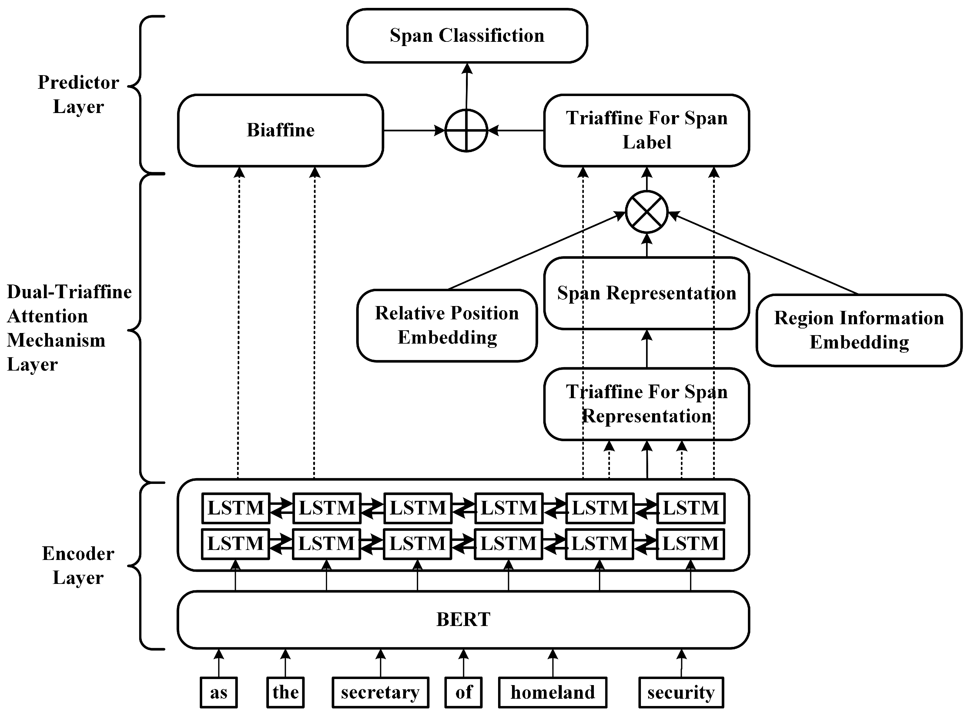
3. Model

This paper proposes a nested entity recognition model that fuses span relative position and region information. The model is mainly composed of three parts: an encoding layer, a dual-triaffine attention mechanism layer, and a predictor layer, as shown in Figure 2. The output of the LSTM goes through two mappings to represent the beginning and the end of the span, which are then used as partial inputs to the biaffine and two triaffine attention modules (shown as dashed lines). The basic idea of the overall model is described as follows:

1. In the encoding layer, the pre-trained language model BERT and Bi-LSTM are used as an encoder to generate word representations containing contextual information from the input sentence.

2. In the dual-triaffine attention mechanism layer, the span representation is generated using one triaffine attention. Then, the obtained span representation is fused with the relative position information and region information. The other triaffine attention is used to interact with the span boundary and the fused information at a high order to obtain a new span representation, which provides a basis for the subsequent span classification.

3. In the predictor layer, all entity span scores are inferred jointly using the predicted values of the triaffine attention mechanisms and the predicted values of the biaffine mechanism.

3.1. Encoder Layer

BERT [30] is adopted as a feature extraction module in the encoder layer. Given a sentence $x=\left\{x_1,x_2,\dots ,x_n\right\}$, $x_i$ represents the i-th word in a sentence. To process the input for BERT, a combination of word embedding vectors, segmentation embedding vectors, and position encoding vectors is used. This means that each word in a sentence may have vectorial representations from multiple pieces after a BERT calculation. To obtain word representations based on the piece representations, we employ a max pooling technique. To further improve context modeling, we utilize a bi-directional LSTM [1], which has been used in previous studies, to generate the final word representations.

$$\mathbf{H}=\left\{{\mathbf{h}}_1,{\mathbf{h}}_2,\cdots ,{\mathbf{h}}_N\right\}\in {\mathbb{R}}^{N\times d_h}$$

(1)

where $d_h$ denotes the dimension of a word representation and N denotes the length of the sentence.

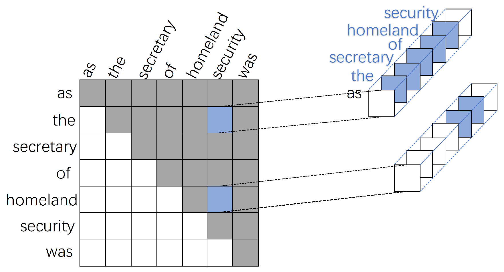
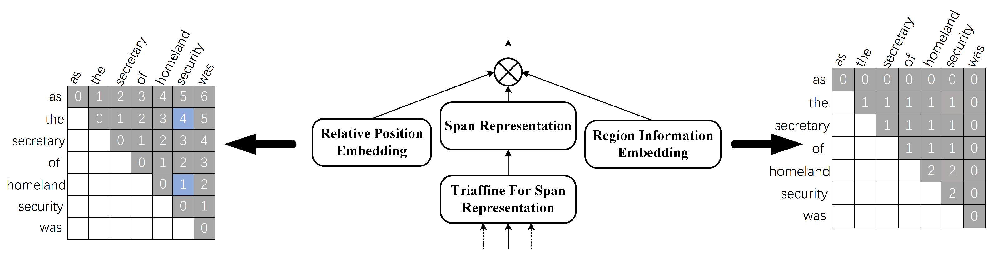
3.2. Dual-Triaffine Attention Mechanism Layer

3.2.1. Triaffine Transformation

The triaffine transformation requires three vectors $\mathbf{u},\mathbf{v},\mathbf{w}\in {\mathbb{R}}^d$ and a parameter tensor $\mathcal{W}\in {\mathbb{R}}^{d+1}\times {\mathbb{R}}^d\times {\mathbb{R}}^{d+1}$ as input vectors, and outputs a scalar, in which distinct MLP (Multi-Layer Perceptron) transformations are applied on input vectors, and tensor vector multiplications are obtained. The constant 1 is concatenated with input vectors, preserving the biaffine transformation, as shown in Equations (2)–(4).

$${\mathbf{u}}^{\prime }=\left[{\mathrm{MLP}}_a\left(\mathbf{u}\right);1\right],{\mathbf{v}}^{\prime }=\left[{\mathrm{MLP}}_c\left(\mathbf{v}\right);1\right]$$

(2)

$${\mathbf{w}}^{\prime }={\mathrm{MLP}}_b\left(\mathbf{w}\right)$$

(3)

$$TriAff\left(\mathbf{u},\mathbf{v},\mathbf{w},\mathcal{W}\right)=\mathcal{W}\times {\mathbf{u}}^{\prime }\times {\mathbf{v}}^{\prime }\times {\mathbf{w}}^{\prime }$$

(4)

where ${\mathrm{MLP}}_t$ stands for t-layer MLP. The tensor initialization conforms to the normal distribution. In the triaffine transformation process, the span boundary representation is denoted as ${\mathbf{u}}^{\prime }$ and ${\mathbf{v}}^{\prime }$, the span internal representation as ${\mathbf{w}}^{\prime }$, and the tensor in the triaffine attention is denoted as $\mathcal{W}$.

3.2.2. Dual-Triaffine Attention Mechanisms

The triaffine attention mechanism layer is divided into two stages. In the first stage, triaffine attention is used to obtain the span representation [14]. In the second stage, the obtained span representation is fused with the relative distance of the entity boundary and the region information within the span. The other triaffine attention is used to generate the label-level span representation again.

(1) Stage one: triaffine attention for span representation

The triaffine attention is used to realize the interaction between the entity span representation and the entity boundary. By introducing the third dimension, the triaffine attention ${\alpha }_{i,j,k,d_m}$ is used to calculate the entity span representation $h_{i,j,d_m}$ of the span $(i,j)$:

$$s_{i,j,k,d_m}=TriAff\left({\mathbf{h}}_i,{\mathbf{h}}_j,{\mathbf{h}}_k,{\mathcal{W}}_{d_m}\right)$$

(5)

$${\alpha }_{i,j,k,d_m}=\frac{exp\left(s_{i,j,k,d_m}\right)}{{\sum }_{k^{\prime }=i}^{j}exp\left(s_{i,j,k^{\prime },d_m}\right)}$$

(6)

$${\mathbf{h}}_{i,j,d_m}=\sum _{k=i}^j{\alpha }_{i,j,k,d_m}\mathrm{MLP}\left({\mathbf{h}}_k\right)$$

(7)

Equations (5)–(7) denote the triaffine attention computation process. The span boundary $({\mathbf{h}}_i,{\mathbf{h}}_j)$ and the embedding dimension parameters $\left({\mathcal{W}}_{d_m}\right)$ are viewed as attention Q (queries), and each word can be viewed as the K (keys) and V (values). This attention mechanism allows Q and K to interact in higher dimensions compared to general attention.

(2) Stage two: fusing location information and region information for span classification

In order to enrich the information of the span grid, we introduce the relative position information of the span boundary and the region information within the span representation, as shown in Figure 3. The left side of the figure shows the relative position information of the word pair grid. In the span grid with row start position and column end position, the distance of an entity from the start position to the end position is the relative position information. In Figure 3, for the entity “the secretary of homeland security”, the distance from “the” to “security” is 4. The right side of the figure shows the region information within the span. In this example, the entity “homeland security” is nested within the entity “the secretary of homeland security”, so the region information is 2 in “homeland security” and 1 in the rest of the region information.

We map each number corresponding to the relative position information and region information to a 20-dimensional vector, represented respectively as ${\mathbf{E}}^d\in {\mathbb{R}}^{N\times N\times d_{E_d}}$ and ${\mathbf{E}}^r\in {\mathbb{R}}^{N\times N\times d_{E_r}}$, where $d_{E_d}$ and $d_{E_r}$ are both equal to 20. We also use ${\mathbf{h}}_{i,j,d_m}\in {\mathbb{R}}^{N\times N\times d_m}$ as the entity span representation. These three vectors are concatenated along the third dimension, as shown in Equation (8):

$${\mathbf{S}}_{i,j,d}=\left[{\mathbf{h}}_{i,j,d_m};{\mathbf{E}}^d;{\mathbf{E}}^r\right]$$

(8)

where $d=d_m+d_{E_d}+d_{E_r},d_m$ denotes the span representation dimension,$d_{E_d}$ denotes the span boundary relative position embedding dimension, and $d_{E_r}$ denotes the span region information embedding dimension.

In the second stage, the output of LSTM is mapped to the span boundary representation ${\mathbf{h}}_{i^{\prime }}{\mathbf{h}}_{j^{\prime }}$ again. Then, with the span representation ${\mathbf{S}}_{i,j,d}$ obtained in the first stage, the label-level span representation is obtained using the triaffine attention, as shown in Equation (9):

$${\mathbf{p}}_{i,j,d^{\prime }}=\mathrm{T}\mathrm{r}\mathrm{i}\mathrm{A}\mathrm{f}\mathrm{f}\left({\mathbf{h}}_{i^{\prime }},{\mathbf{h}}_{j^{\prime }},{\mathbf{S}}_{i,j,d},{\mathcal{V}}_{d^{\prime }}\right)$$

(9)

Similarly to the procedure described in the first stage, the span boundary and the label are used as Q for the attention mechanism. Span is represented as attention K (keys) and V (values) to obtain the label-level span representation ${\mathbf{p}}_{i,j,d^{\prime }}$.

3.3. Predictor Layer

After the label-level span representation is obtained, we use the label-level span representation of the output of the second stage as one predictor and the biaffine mechanism as the other to compute two independent relational distributions of the span ($x_i$,$x_j$), where $x_i$ and $x_j$ represent the head and tail of the span, respectively. The results of these calculations are combined as the final prediction score.

3.3.1. Span Prediction

Based on the label-level span representation ${\mathbf{p}}_{i,j,d^{\prime }}$ obtained by the triaffine attention mechanism, we use an MLP to calculate the score of the span from the i-th word to the j-th word, as shown in Equation (10):

$${\mathbf{y}}_{i,j}^{″}=\mathrm{M}\mathrm{L}\mathrm{P}\left({\mathbf{p}}_{i,j,d^{\prime }}\right)$$

(10)

3.3.2. Biaffine Prediction

The input to the biaffine predictor is the output of the encoding layer. For a given sentence of length N, two MLPs are used to compute the head ${\mathbf{s}}_i$ and tail ${\mathbf{t}}_j$ representations of the span (entity), and then a biaffine classifier is used to compute the entity label score for this pair of head and tail ($x_i$,$x_j$), as shown in Equations (11)–(13):

$${\mathbf{s}}_i={\mathrm{MLP}}_1\left({\mathbf{h}}_i\right)$$

(11)

$${\mathbf{t}}_j={\mathrm{MLP}}_2\left({\mathbf{h}}_j\right)$$

(12)

$${\mathbf{y}}_{i,j}^{\prime }={{\mathbf{s}}_i}^T\mathbf{U}{\mathbf{t}}_j+\mathbf{W}\left[{\mathbf{s}}_i;{\mathbf{t}}_j\right]+\mathbf{b}$$

(13)

where $\mathbf{U}$,$\mathbf{W}$,$\mathbf{b}$ are learnable parameters, ${\mathbf{s}}_i$ and ${\mathbf{t}}_j$ denote the head and tail representation of the span ($x_i$,$x_j$), and $y_{i,j}^{\prime }$ represents the label score.

The final span label probability is obtained by combining the scores of the span predictor and the biaffine predictor, as shown in Equation (14):

$${\mathbf{y}}_{i,j}=\mathrm{Softmax}\left({\mathbf{y}}_{i,j}^{\prime }+{\mathbf{y}}_{i,j}^{″}\right)$$

(14)

3.4. Loss Function

For a sentence, the objective function for model training is to minimize the log-likelihood loss with respect to the corresponding label, which is formulated as shown in Equation (15):

$$\mathcal{L}=-\frac{2}{N\left(N+1\right)}\sum _{i=1}^N\sum _{j=1}^i\sum _{l=1}^L{\widehat{\mathbf{y}}}_{i,j}^{l}log{\mathbf{y}}_{i,j}^l$$

(15)

where N denotes the number of words in the sentence, ${\widehat{\mathbf{y}}}_{i,j}^l$ denotes the true label of the span ($x_i$,$x_j$), ${\mathbf{y}}_{i,j}^l$ denotes the predicted value, and l denotes the l-th label in the label set L. Because only the upper triangle region is valid in the span table, the loss is calculated in such a way that only the upper triangle is calculated.

4. Experiment and Analysis

4.1. Dataset

We conducted experiments using the ACE2004, ACE2005, and GENIA datasets. The ACE2004 and ACE2005 datasets are divided into train/test/validation subsets with a ratio of 8:1:1 according to the method proposed by Shibuya and Hovy [6]. The GENIA dataset is divided into train/test subsets with an 8:2 ratio according to the method proposed by Zheng Yuan et al. [14]. To verify the performance of the model, we also conducted experiments on the flat entity dataset resume [31], using precision P, recall R, and F1 score to represent the model performance. The numbers of entities in the above four datasets are shown in

Table 1. Statistics on the numbers of dataset entities.

	ACE2004			ACE2005			GENIA		Resume
	Train	Dev	Test	Train	Dev	Test	Train	Test	Train	Dev	Test
Sentences	6198	742	809	7285	968	1058	16,692	1854	36,487	6083	4472
Entities	22,204	2514	3035	24,827	3234	3041	50,509	5506	61,726	8969	7378
Nested entities	10148	1090	1415	9389	1110	1120	9064	1199

Note: The Resume dataset is a flat dataset, so there are no nested entities.

.

4.2. Experiment Details

For the datasets ACE2004 and ACE2005, we use BERT-large-uncased as a contextual embedding method with a learning rate of 1 × 10${}^{-5}$. For the dataset GENIA, we use Bio-BERT-v1.1 as a text context embedding method with a learning rate of 1 × 10${}^{-6}$. The BiLSTM with a hidden size of 1024 is used for the token representations for the ACE2004 and ACE2005 datasets, and 512 is used for the token representations for the GENIA dataset. The dimension of the triaffine span representation is 512. The distance embedding dimension $d_{E_d}$ is 20, the region information embedding dimension $d_{E_r}$ is 20, the biaffine dimension of the predictor layer is 1024, and the learning rate of the remaining model parameters is 1 × 10${}^{-3}$.

The parameters are mainly determined by the size of the hidden layer dimension in the pre-training model and the content of the dataset. The ACE datasets are publicly available. The hidden layer dimension of the widely used pre-training model is 1024, which indicates that the hidden layer dimension of the LSTM layer will also be relatively large. The GENIA dataset is a specialized biomedical corpus. The size of the dataset is small, the hidden layer dimension of the pre-trained model is 768, and the hidden layer dimension in the LSTM layer will be relatively small, as shown in

Table 2. Experimental parameters.

Parameter Types	ACE2004, ACE2005	GENIA
BERT name	BERT-large-uncased	BioBERT-v1.1
BERT learning rate	1 × 10${}^{-5}$	1 × 10${}^{-6}$
BERT hidden size	1024	768
LSTM hidden size	1024	512
Triaffine hidden size	512	512
Epoch	50	35
Embedding dropout	0.5	0.3
Out dropout	0.2	0.2
Batch size	8	8
Distance embedding size $d_{E_d}$	20	20
Region embedding size $d_{E_r}$	20	20
Learning rate	1 × 10${}^{-3}$	1 × 10${}^{-3}$
Optimizer	AdamW	AdamW

.

4.3. Baseline Approaches

There are a total of nine baseline approaches considered in previous studies. Yuan et al. [14] proposed a triaffine mechanism that calculates the score of entities based on span and label information. Yu et al. [15] utilized a biaffine function to determine the entity boundary and performed classification on the identified span. Xia et al. [16] developed a detector to screen candidate entity spans and used a classifier for classification purposes. Luan et al. [19] employed a multi-task learning approach to extract entities and relations simultaneously. Fu et al. [27] treated entities as nodes in a constituency tree and used a masking internal algorithm for decoding. Straková et al. [11] utilized a sequence-to-sequence approach for nested entity extraction. Wang et al. [3] introduced a pyramid layer and an inverse pyramid layer for decoding nested entities. Shibuya et al. [6] applied multiple CRFs in an outside-to-inside layer-wise manner for nested entity extraction. Tan et al. [13] proposed a boundary-enhanced neural span classification model and introduced an additional boundary detection method based on span classification to predict entity boundaries.

4.4. Experimental Results and Analysis

4.4.1. Experiments on the Nested Entity Datasets

The results on the three nested entity datasets, ACE2004, ACE2005 and GENIA, are presented in

Table 3. Experimental results on ACE2004, ACE2005 and GENIA datasets.

Method	ACE2004			ACE2005			GENIA
	P	R	F1	P	R	F1		P	R	F1
Luan et al. [19]	-	-	84.7	-	-	82.9	BERT	-	-	76.2
Xia et al. [16]	81.7	77.4	79.5	79.0	77.3	78.2	BERT	-	-	-
Tan et al. [13]	85.8	84.8	85.3	83.8	83.9	83.9	BERT	79.2	77.4	78.3
Fu et al. [27]	86.7	86.5	86.6	84.5	86.4	85.4	BERT	78.2	78.2	78.2
Yu et al. [15]	87.3	86.0	86.7	85.2	85.6	85.4	BERT	81.8	79.3	80.5
Wang et al. [3]	86.08	86.48	86.28	83.95	85.39	84.66	Bio-BERT	79.63	78.38	79.00
Straková et al. [11]	84.71	83.96	84.33	82.58	84.29	83.42	BERT	79.92	76.55	78.20
Shibuya et al. [6]	85.23	84.72	84.97	83.30	84.69	83.99	BERT	77.46	76.65	77.05
Yuan et al. [14]	87.13	87.68	87.40	86.70	86.94	86.82	Bio-BERT	80.42	82.06	81.23
Ours	87.91	87.41	87.66	85.80	87.95	86.86	Bio-BERT	83.02	78.88	80.90

. Compared with the nine baseline approaches, our model achieves suboptimal results on the GENIA dataset and achieves optimal results on the other two datasets. The F1 values of our model on the ACE2004 and ACE2005 datasets reach 87.66% and 86.86%, respectively; these results are better than those of other methods based on span [14,15,16,19] and Seq2Seq [11]. Compared with the best method in Yuan et al.’s work [14], the F1 values are increased by 0.26% and 0.04%, respectively.

For the GENIA dataset, the F1 value of our model is 0.33, which is lower than that of Yuan et al.’s model [14]. In their model, when word vectors are generated, for each sentence, the target sentence and its previous and next sentences are fed into BERT and Bi-LSTM together to obtain better contextual embedding. Yuan et al.’s model is more beneficial to the word vector representation of biomedical corpora such as GENIA. However, the number of parameters in their model is large, and the training time is long.

For a fair comparison with Yuan et al.’s model [14], in the process of generating the contextual embedding, we abandon the previous and next sentences of the target sentence. We only use the target sentence as an input.

Table 4. Comparison of model effects based on single-sentence input condition.

	GENIA		ACE2004
	Yuan et al. [14]	Ours	Yuan et al. [14]	Ours
Total Parameters	526,495,078	255,976,987	628,675,700	524,412,639
Batch Size	4	4	4	4
BERT	Bio-BERT	Bio-BERT	BERT-large-uncased	BERT-large-uncased
Train Time (one epoch)	17 min	7 min	6 min	3.5 min
GPU Memory	30 G	19 G	30 G	30 G
LSTM Hidden Size	1024	512	1024	1024
F1 score	80.33	80.90	87.11	87.66

shows the results of the comparison in terms of F1 score, parameter quantity, and training time on the GENIA and ACE2004 datasets. Under the same conditions, the F1 score of our model is higher than that of Yuan et al.’s model, and the training time and the number of parameters are relatively small. The specific parameters can be referred to in Table 2.

4.4.2. Experiments on the Flat Entity Datasets

In order to verify the performance of our model, we also conducted experiments on the flat dataset, Resume. Based on the results given in

Table 5. Experimental results on the Resume dataset.

	Resume
	P	R	F1
Yan et al. (2019) [23]	-	-	95.00
Gui et al. (2019) [32]	95.37	94.84	95.11
Li et al. (2020) [24]	-	-	95.86
Ma et al. (2020) [33]	96.08	96.13	96.13
Li et al. (2022) [28]	96.96	96.35	96.65
Ours	95.77	96.73	96.24

, our model achieves a higher performance than most of the current studies. Compared with Li et al.’s model [28], our model achieves a lower F1 score because the entity representation dimension of our triaffine attention mechanism is too high. Flat entities are distributed more sparsely than nested entities, which produces sparse entity features, resulting in a performance decline.

4.5. Ablation Experiments

Ablation experiments were carried out on the ACE2005 dataset. The results are shown in

Table 6. Model ablation experiment.

	ACE2005
	P	R	F1
case1	83.65	87.82	85.65 (−1.21)
case2	85.48	86.33	85.90 (−0.96)
case3	85.10	87.49	86.28 (−0.58)
case4	85.36	87.59	86.46 (−0.4)
Full model	85.80	87.95	86.86

. Without the dual-triaffine attention mechanism layer, the biaffine prediction (case1) is directly used after the context embedding obtained by BERT. The performance is reduced by 1.21%. After both the relative position information embedding and region information embedding are removed, the model contains only one stage of this span representation (case2). The performance is decreased by 0.96%. After the relative position information embedding of the span boundary (case3) is removed, the performance is decreased by 0.58%. After the information embedding of the region within the span (case4) is removed, the performance is decreased by 0.4%.

4.6. Discussion

In this section, we will discuss our model using specific example sentences. In the sentence a ’new york times’ reporter lends cook his mobile sat phone the phrase a ’new york times’ reporter belongs to the person type, and new york times belongs to the organization type. Taking “a ’new york times’ reporter” as an example, the biaffine module makes judgments based on the word embedding information of a and reporter, while the triaffine module incorporates the word embedding information of the entire span a ’new york times’ reporter into the word pair table. The relative position information of this entity is 6. a, and reporter are within one entity, with a region information value of 1. new york and times are within two entities, with a region information value of 2. Distance information and region information are mapped to 20-dimensional vectors and incorporated into the model calculation. In this way, the model can learn the boundary information of spans of any length and the information within the spans. By considering multiple dimensions of information, the model can make more accurate predictions for entity recognition.

We have also learned some lessons from the experiments. More complex models may have stronger fitting capabilities, but they may also be more prone to over-fitting or require more computational resources. This could impose limitations on computational efficiency, model deployment, and scalability in practical applications. Additionally, when the model encounters data from specific professional domains, the performance may not be ideal.

5. Conclusions

This paper proposes a span-based nested entity recognition model. The model utilizes a pre-trained module and LSTM encoding approach, and incorporates a triaffine attention mechanism for entity span representation. The span representation is then fused with relative position and region information, and another triaffine attention is applied to generate the entity representation. The outputs of the triaffine attention and biaffine mechanisms are jointly used for predicting and classifying entity spans. Experimental results demonstrate that our model achieves state-of-the-art performance on three widely used datasets. Ablation experiments indicate that the inclusion of a dual triaffine attention, which integrates relative position and region information, enhances nested entity recognition. Additionally, we recognize the limitations of the model’s generalization capability and the trade-off between model complexity and performance. In the future, we will continuously optimize the model to improve its performance and explore the application of triaffine transformation on discontinuous entity datasets.

References

- Lample, G.; Ballesteros, M.; Subramanian, S. Neural architectures for named entity recognition. arXiv 2016, arXiv:1603.01360. [Google Scholar]
- Yuan, Z.; Liu, Y.; Yin, Q. Unsupervised multi-granular Chinese word segmentation and term discovery via graph partition. J. Biomed. Inform. 2020, 110, 103542. [Google Scholar] [CrossRef] [PubMed]
- Wang, J.; Shou, L.; Chen, K. Pyramid: A layered model for nested named entity recognition. In Proceedings of the 58th Annual Meeting of the Association for Computational Linguistics, Online, 5–10 July 2020; pp. 5918–5928. [Google Scholar]
- Ju, M.; Miwa, M.; Ananiadou, S. A neural layered model for nested named entity recognition. In Proceedings of the 2018 Conference of the North American Chapter of the Association for Computational Linguistics: Human Language Technologies, New Orleans, LA, USA, 1–6 June 2018; pp. 1446–1459. [Google Scholar]
- Fisher, J.; Vlachos, A. Merge and label: A novel neural network architecture for nested NER. arXiv 2019, arXiv:1907.00464. [Google Scholar]
- Shibuya, T.; Hovy, E. Nested named entity recognition via second-best sequence learning and decoding. Trans. Assoc. Comput. Linguist. 2020, 8, 605–620. [Google Scholar] [CrossRef]
- Muis, A.O.; Lu, W. Learning to recognize discontiguous entities. arXiv 2018, arXiv:1810.08579. [Google Scholar]
- Katiyar, A.; Cardie, C. Nested named entity recognition revisited. In Proceedings of the 2018 Conference of the North American Chapter of the Association for Computational Linguistics: Human Language Technologies, New Orleans, LA, USA, 1–6 June 2018; pp. 861–871. [Google Scholar]
- Wang, B.; Lu, W. Neural segmental hypergraphs for overlapping mention recognition. arXiv 2018, arXiv:1810.01817. [Google Scholar]
- Gillick, D.; Brunk, C.; Vinyals, O. Multilingual language processing from bytes. arXiv 2015, arXiv:1512.00103. [Google Scholar]
- Straková, J.; Straka, M.; Hajič, J. Neural architectures for nested NER through linearization. arXiv 2019, arXiv:1908.06926. [Google Scholar]
- Zheng, C.; Cai, Y.; Xu, J. A boundary-aware neural model for nested named entity recognition. In Proceedings of the 2019 Conference on Empirical Methods in Natural Language Processing and the 9th International Joint Conference on Natural Language Processing (EMNLP-IJCNLP), Hong Kong, China, 3–7 November 2019; pp. 357–366. [Google Scholar]
- Tan, C.; Qiu, W.; Chen, M. Boundary enhanced neural span classification for nested named entity recognition. In Proceedings of the AAAI Conference on Artificial Intelligence, New York, NY, USA, 7–12 February 2020; Volume 34, pp. 9016–9023. [Google Scholar]
- Yuan, Z.; Tan, C.; Huang, S. Fusing heterogeneous factors with triaffine mechanism for nested named entity recognition. arXiv 2021, arXiv:2110.07480. [Google Scholar]
- Yu, J.; Bohnet, B.; Poesio, M. Named entity recognition as dependency parsing. arXiv 2020, arXiv:2005.07150. [Google Scholar]
- Xia, C.; Zhang, C.; Yang, T.; Li, Y.; Du, N.; Wu, X.; Fan, W.; Ma, F.; Yu, P. Multi-grained Named Entity Recognition. In Proceedings of the 57th Annual Meeting of the Association for Computational Linguistics, Florence, Italy, 28 July–2 August 2019. [Google Scholar]
- Wadden, D.; Wennberg, U.; Luan, Y.; Hajishirzi, H. Entity, Relation, and Event Extraction with Contextualized Span Representations. In Proceedings of the 2019 Conference on Empirical Methods in Natural Language Processing and the 9th International Joint Conference on Natural Language Processing (EMNLP-IJCNLP), Hong Kong, China, 3–7 November 2019. [Google Scholar]
- Zhong, Z.; Chen, D. A Frustratingly Easy Approach for Entity and Relation Extraction. In Proceedings of the 2021 Conference of the North American Chapter of the Association for Computational Linguistics: Human Language Technologies, Online, 6–11 June 2021. [Google Scholar]
- Luan, Y.; Wadden, D.; He, L.; Shah, A.; Ostendorf, M.; Hajishirzi, H. A general framework for information extraction using dynamic span graphs. In Proceedings of the 2019 Conference of the North American Chapter of the Association for Computational Linguistics: Human Language Technologies, Volume 1 (Long and Short Papers), Minneapolis, MN, USA, 2–7 June 2019. [Google Scholar]
- Lafferty, J.; McCallum, A.; Pereira, F.C. Conditional Random Fields: Probabilistic Models for Segmenting and Labeling Sequence Data. In Proceedings of the Eighteenth International Conference on Machine Learning, San Francisco, CA, USA, 28 June–1 July 2001. [Google Scholar]
- Ronan, C.; Jason, W.; Léon, B.; Michael, K.; Koray, K.; Pavel, P.K. Natural Language Processing (almost) from Scratch. J. Mach. Learn. Res. 2011, 12, 2493–2537. [Google Scholar]
- Strubell, E.; Verga, P.; Belanger, D.; McCallum, A. Fast and Accurate Entity Recognition with Iterated Dilated Convolutions; Association for Computational Linguistics: Copenhagen, Denmark, 2017; pp. 2670–2680. [Google Scholar]
- Yan, H.; Deng, B.; Li, X.; Qiu, X. TENER: Adapting Transformer Encoder for Named Entity Recognition. arXiv 2019, arXiv:1911.04474. [Google Scholar]
- Li, X.; Yan, H.; Qiu, X.; Huang, X. FLAT: Chinese NER Using Flat-Lattice Transformer. In Proceedings of the 58th Annual Meeting of the Association for Computational Linguistics, Online, 5–10 July 2020; pp. 6836–6842. [Google Scholar]
- Yan, H.; Gui, T.; Dai, J.; Guo, Q.; Zhang, Z.; Qiu, X. A Unified Generative Framework for Various NER Subtasks. In Proceedings of the 59th Annual Meeting of the Association for Computational Linguistics and the 11th International Joint Conference on Natural Language Processing (Volume 1: Long Papers), Online, 1–6 August 2021; pp. 5808–5822. [Google Scholar]
- Lewis, M.; Liu, Y.; Goyal, N.; Ghazvininejad, M.; Mohamed, A.; Levy, O.; Stoyanov, V.; Zettlemoyer, L. BART: Denoising Sequence-to-Sequence Pre-training for Natural Language Generation, Translation, and Comprehension. In Proceedings of the 58th Annual Meeting of the Association for Computational Linguistics, Online, 5–10 July 2020; pp. 7871–7880. [Google Scholar]
- Fu, Y.; Tan, C.; Chen, M.; Huang, S.; Huang, F. Nested Named Entity Recognition with Partially-Observed TreeCRFs. In Proceedings of the AAAI Conference on Artificial Intelligence, Virtually, 2–9 February 2021; pp. 12839–12847. [Google Scholar]
- Li, J.; Fei, H.; Liu, J.; Wu, S.; Zhang, M.; Teng, C.; Ji, D.; Li, F. Unified Named Entity Recognition as Word-Word Relation Classification. In Proceedings of the AAAI Conference on Artificial Intelligence, Vancouver, BC, Canada, 22 February–1 March 2022; pp. 10965–10973. [Google Scholar]
- Li, J.; Xu, K.; Li, F.; Fei, H.; Ren, Y.; Ji, D. MRN: A Locally and Globally Mention-Based Reasoning Network for Document-Level Relation Extraction. In Proceedings of the Findings of the Association for Computational Linguistics: ACL-IJCNLP 2021, Online, 1–6 August 2021; pp. 1359–1370. [Google Scholar]
- Devlin, J.; Chang, M.; Lee, K.; Toutanova, K. BERT: Pre-training of Deep Bidirectional Transformers for Language Understanding. In Proceedings of the 2019 Conference of the North American Chapter of the Association for Computational Linguistics: Human Language Technologies, Volume 1 (Long and Short Papers), Minneapolis, MN, USA, 2–7 June 2019; pp. 4171–4186. [Google Scholar]
- Zhang, Y.; Yang, J. Chinese NER Using Lattice LSTM. In Proceedings of the 56th Annual Meeting of the Association for Computational Linguistics (Volume 1: Long Papers), Melbourne, Australia, 15–20 July 2018; pp. 1554–1564. [Google Scholar]
- Gui, T.; Zou, Y.; Zhang, Q.; Peng, M.; Fu, J.; Wei, Z.; Huang, X. A Lexicon-Based Graph Neural Network for Chinese NER. In Proceedings of the 2019 Conference on Empirical Methods in Natural Language Processing and the 9th International Joint Conference on Natural Language Processing (EMNLP-IJCNLP), Hong Kong, China, 3–7 November 2019; pp. 1040–1050. [Google Scholar]
- Ma, R.; Peng, M.; Zhang, Q.; Huang, X. Simplify the Usage of Lexicon in Chinese NER. In Proceedings of the 58th Annual Meeting of the Association for Computational Linguistics, Online, 5–10 July 2020; pp. 5951–5960. [Google Scholar]