Noisy Quantum Channel Characterization Using Quantum Neural Networks

Abstract

Channel noise is considered to be the main obstacle in long-distance quantum communication and distributed quantum networks. Here, employing a quantum neural network, we present an efficient method to study the model and detect the noise of quantum channels. Based on various types of noisy quantum channel models, we construct the architecture of the quantum neural network and the model training process. Finally, we perform experiments to verify the training effectiveness of the scheme, and the results show that the cost function of the quantum neural network could approach above 90% of the channel model.

1. Introduction

Quantum information processing is the transmission or processing of information through a quantum system [1,2], such as quantum communications [3,4,5,6,7], quantum computation [8,9,10] and quantum metrology [11,12]. During recent decades, there have been extensive studies into quantum information processing. Specifically, quantum communications (QC), as the most promising approach for secure information transmission, is becoming increasingly applicable. In the realization of QC, the quantum channels are key ingredients for quantum information and signal transmission. However, there are two main obstacles in the channels for the implementation of long-distance communications and network construction: channel loss and channel noise [13]. There are many related works on eliminating channel noise, such as channel discrimination [14], error-rejection coding [15] and quantum error corrections [16,17,18]. As a priority in the research of noisy quantum communications, noisy quantum channel detection is perceived as a highly versatile task.

Meanwhile, classical and quantum neural networks have become pervasive tools in quantum information processing [19,20]. During recent decades, intensive research work related to quantum neural networks has made great progress, and the applications of quantum neural networks in various quantum information tasks have also gradually increased with their increased performances [21,22,23,24]. For example, in 2010, Bisio et al. focused on storing the unitary operation in a quantum memory with limited resources rather than improving their performance and generalization [25]. In ref. [26], Verdon et al. introduced quantum machine learning of parametrized unitary operations and proved that it is possible to construct a functionally simpler linear quantum perceptron to fit the unitary mapping. Based on this work, Beer et al. used the unitary operator as a quantum perceptron and proposed a corresponding efficient training algorithm [27]. The quantum perceptrons form a quantum neural network through connections, which can achieve forward propagation and back propagation and complete the task of learning arbitrary unknown unitary operators.

In this paper, employing a quantum neural network, we study various noisy channel models of quantum communications to enable a high accuracy information transmission. Meanwhile, the errors caused by channel noise during the information transmission process can be reduced. Numerical experiments are performed to evaluate the performance of the model. By analyzing the experimental results, we conclude that the quantum neural network is effective for both two-dimensional and three-dimensional quantum channels, which can be further generalized to higher-dimensional cases. Among the studies related to improving the performance of the quantum neural network, we find that a simpler structured network works better for simple tasks. Furthermore, the network hyperparameter $\lambda$, which is the reciprocal of the learning rate, is selected according to the problem at hand. The random initialization of the network impacts the training performance, which can be reduced by increasing the number of training rounds.

Our paper is organized as follows: in Section 2, we briefly introduce a model of a noisy quantum channel and a quantum neural network. In Section 3, we feature the details of our scheme including task definition, data preparation, network architecture and the training process. In Section 4, we present our experimental results and analyses. In Section 5, we propose some methods to improve the performance of the network. In Section 6, we test the robustness of the network. Finally, we summarize the work in Section 7.

2. Preliminaries

2.1. Noisy Quantum Channel

Theoretically, the channel noise will cause signal distortion, which affects the efficiency and fidelity of qubits during transmission. Here, in this part, we first present the basic models of noisy quantum channels.

2.1.1. Channel Models under Two-Dimensional Hilbert Space

Traditionally, four basic noisy quantum channels are commonly used in the qubit and are expressed by a two-dimensional Hilbert space. These are called the depolarizing channel, amplitude damping channel, phase damping channel and bit flip channel [28].

• Depolarizing channel.
  The qubits are transmitted through the depolarizing channel, with the probability of the states being unchanged as $1-p$, and the probability, p, that they become completely mixed state as $I/2$. The channel operator can be described by a completely positive trace-preserving map as

  $$\epsilon \left(\rho \right)=\frac{pI}{2}+(1-p)\rho .$$

  (1)

  where $\rho$ represents the input state and the mixed state $I/2$ can be expressed as

  $$\frac{I}{2}=\frac{\rho +{\sigma }_1\rho {\sigma }_1+{\sigma }_2\rho {\sigma }_2+{\sigma }_3\rho {\sigma }_3}{4}.$$

  (2)
  By substituting $I/2$ into the above formula, we get

  $$\epsilon \left(\rho \right)=(1-\frac{3p}{4})\rho +\frac{p}{4}({\sigma }_1\rho {\sigma }_1+{\sigma }_2\rho {\sigma }_2+{\sigma }_3\rho {\sigma }_3).$$

  (3)
  From the above equation, it is obvious that there is a $1-3p/4$ probability of maintaining the original state, and a $p/4$ probability that the input state will undergo the relative ${\sigma }_1$, ${\sigma }_2$ and ${\sigma }_3$ operations. Here, ${\sigma }_1$, ${\sigma }_2$ and ${\sigma }_3$ are the Pauli matrices, expressed as

  $${\sigma }_1={\sigma }_x=\left(\begin{array}{cc}0& 1\\ 1& 0\end{array}\right),{\sigma }_2={\sigma }_y=\left(\begin{array}{cc}0& -i\\ i& 0\end{array}\right),{\sigma }_3={\sigma }_z=\left(\begin{array}{cc}1& 0\\ 0& -1\end{array}\right).$$

  (4)
  The Kraus operators of the depolarizing channel can be obtained by

  $$E_0=\sqrt{1-\frac{3p}{4}}I,E_1=\sqrt{\frac{p}{4}}{\sigma }_x,E_2=\sqrt{\frac{p}{4}}{\sigma }_y,E_3=\sqrt{\frac{p}{4}}{\sigma }_z.$$

  (5)
• Amplitude damping channel.
  The amplitude damping channel describes the energy dissipation of the qubits system, which can be described as

  $$\epsilon \left(\rho \right)=E_0\rho E_0^{†}+E_1\rho E_1^{†}.$$

  (6)
  Here, the normalization condition satisfies the relation

  $$E_0^{†}{E}_0+E_1^{†}{E}_1=1$$

  (7)

  where the Kraus operations $E_0$ and $E_1$ can be expressed as

  $$E_0=\left[\begin{array}{cc}1& 0\\ 0& \sqrt{1-\gamma }\end{array}\right],E_1=\left[\begin{array}{cc}0& \sqrt{\gamma }\\ 0& 0\end{array}\right].$$

  (8)
• Phase damping channel.
  The phase damping channel describes the loss of quantum information without the loss of energy; it has the same expression as $\epsilon \left(\rho \right)$ in the amplitude damping channel, but with different Kraus operations

  $$E_0=\left[\begin{array}{cc}1& 0\\ 0& \sqrt{1-\gamma }\end{array}\right],E_1=\left[\begin{array}{cc}0& 0\\ 0& \sqrt{\gamma }\end{array}\right].$$

  (9)
  The $E_0$ operation leaves $|0\rangle$ unchanged but reduces the amplitude of the $|1\rangle$ state. Furthermore, the $E_1$ operation destroys $|0\rangle$ and reduces the amplitude of the $|1\rangle$ state.
• Bit-flip channel.
  The bit-flip channel keeps the original input state unchanged with the probability p, and flips the state of each qubit from $|0\rangle$($|1\rangle$) to $|1\rangle$ ($|0\rangle$) with the probability $1-p$, which can be described as

  $$\epsilon \left(\rho \right)=p\rho +(1-p)X\rho .$$

  (10)
  Furthermore, it has Kraus operations that can be defined as

  $$E_0=\sqrt{p}I=\sqrt{p}\left[\begin{array}{cc}1& 0\\ 0& 1\end{array}\right],E_1=\sqrt{1-p}X=\sqrt{1-p}\left[\begin{array}{cc}0& 1\\ 1& 0\end{array}\right].$$

  (11)

2.1.2. Channel Models under Three-Dimensional Hilbert Space

To increase the channel capacity, a higher dimensional coding space can also be considered for qutrit transmission. The noisy quantum channel that is commonly used in the qutrit system can be expressed in the general form as

$$U_{mn}=\sum _{j=0}^2{e}^{2\pi ijn/d}|(j+m)\%d\rangle \langle j|.$$

(12)

Here, the parameters $m,n=0,1,2$. Furthermore, the corresponding operators in the above equation can be described as

$$\begin{array}{c}\hfill U_{00}=\left[\begin{array}{ccc}1& 0& 0\\ 0& 1& 0\\ 0& 0& 1\end{array}\right],U_{01}=\left[\begin{array}{ccc}1& 0& 0\\ 0& e^{2\pi i/3}& 0\\ 0& 0& e^{4\pi i/3}\end{array}\right],U_{02}=\left[\begin{array}{ccc}1& 0& 0\\ 0& e^{4\pi i/3}& 0\\ 0& 0& e^{8\pi i/3}\end{array}\right],\\ \\ \hfill U_{10}=\left[\begin{array}{ccc}0& 0& 1\\ 1& 0& 0\\ 0& 1& 0\end{array}\right],U_{11}=\left[\begin{array}{ccc}0& 0& e^{4\pi i/3}\\ 1& 0& 0\\ 0& e^{2\pi i/3}& 0\end{array}\right],U_{12}=\left[\begin{array}{ccc}0& 0& e^{8\pi i/3}\\ 1& 0& 0\\ 0& e^{4\pi i/3}& 0\end{array}\right],\\ \\ \hfill U_{20}=\left[\begin{array}{ccc}0& 1& 0\\ 0& 0& 1\\ 1& 0& 0\end{array}\right],U_{21}=\left[\begin{array}{ccc}0& e^{2\pi i/3}& 0\\ 0& 0& e^{4\pi i/3}\\ 1& 0& 0\end{array}\right],U_{22}=\left[\begin{array}{ccc}0& e^{4\pi i/3}& 0\\ 0& 0& e^{8\pi i/3}\\ 1& 0& 0\end{array}\right].\end{array}$$

(13)

Then, according to Euler’s equation, $e^{ix}=cosx+isinx$, an approximation of U can be obtained.

2.2. Quantum Neural Network

Quantum neural networks realize the basic structure of a neural network by considering the dynamics of quantum mechanics, which uses quantum memory and computing power advantages to achieve more efficient and smarter learning abilities. The quantum neural networks in this work use a general unitary operator as a quantum perceptron, this operator can only process quantum data and the transformations of quantum gates on quantum information that is unitary and linear. Quantum neurons can be mathematically represented as matrices, and the process of training quantum neural networks can be interpreted as iteratively adjusting the matrix values to improve the network’s ability to fit the input data.

A quantum neural network has a similar workflow to a classical neural network in terms of processing data, including task definition, data preparation, data preprocessing, training the network, optimizing the parameters, testing the network performance and selecting the optimal result. To achieve the detection of noisy quantum channels for quantum neural networks, the quantum neural network needs to learn a general detection method, whether for 2D or 3D noisy channels.

3. Methodology

3.1. Task Definition

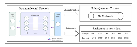
The aim of this work is to employ quantum neural networks to identify and characterize the impact of noisy quantum channels, enabling the trained networks to replicate the effects of quantum noise channels. Before training starts, we need to finish the preparation steps, including data preparation, model building and parameter initialization. Then, we can realize the transmission of information by performing forward propagation and obtain the output states of the network. Through calculating the fidelity between the network’s output states and the output states in the data, we can obtain the cost function between them. If the current result does not satisfy the end condition, the unitary operation of the network is updated by the back propagation algorithm. The training procedure described above can be depicted in Figure 1. After training is finished, we can use the test data to evaluate the performance of the quantum neural networks. Furthermore, by adjusting the structure and other parameters of the networks, the network structure with the best performance can be selected.

3.2. Data Preparation

The data preparation in this work includes two subsections: preparation of the noisy quantum channel and preparation of the training data. The former outlines the steps taken to simulate a quantum channel with added noise, while the latter describes the generation of the input and target data for the neural network.

3.2.1. Preparation of the Noisy Quantum Channel

In practical applications, the form of the noisy quantum channel is always unknown. Thus, in this work, we simulate the noisy quantum channel by initializing it in a random form. As the form of the generated noisy quantum channel is unknown to the quantum neural network, it will not have any effect on training.

Taking the four channels in two-dimensional Hilbert space as an example, the preparation process for each noisy quantum channel can be described as follows:

• It is required to generate the parameters p and $\gamma$ in the expression randomly which take a value in $(0,1)$.
• Each Kraus operation of the channel is assigned a weight w with a value in $(0,1)$, then we obtain the value E of the channel as

  $$E=\sum _{i=1}^n{w}_i{e}_i,$$

  (14)

  where $w_i$ denotes the probability of occurrence of the i-th Kraus operation, $e_i$ is the value of i-th Kraus operation, n represents the number of Kraus operations in the channel and ${\sum }_{i=1}^n{w}_i=1$.

3.2.2. Preparation of the Training Data

According to the requirements of the quantum neural network model, the training data consist of pairs of a combination of input states and output states, which can be defined as

$$D_{train}=\{({\mathsf{\Psi }}_{in}^1,{\mathsf{\Psi }}_{out}^1),({\mathsf{\Psi }}_{in}^2,{\mathsf{\Psi }}_{out}^2),\cdots ,({\mathsf{\Psi }}_{in}^n,{\mathsf{\Psi }}_{out}^n)\},$$

(15)

where ${\mathsf{\Psi }}_{in}$ represents the input state, which is a normalized pure state generated randomly. The output state through the noisy quantum channel E can be described as $|{\mathsf{\Psi }}_{out}\rangle =E|{\mathsf{\Psi }}_{in}\rangle$.

According to the definition of the cost function, the states need to be normalized to ensure that the calculated fidelity value is between 0 and 1. Thus, the output state should be normalized, i.e., $|{\mathsf{\Psi }}_{out}\rangle =Norm\left(\right|{\mathsf{\Psi }}_{out}\rangle )$. After that, the training data are divided into two sets: the training set and the test set.

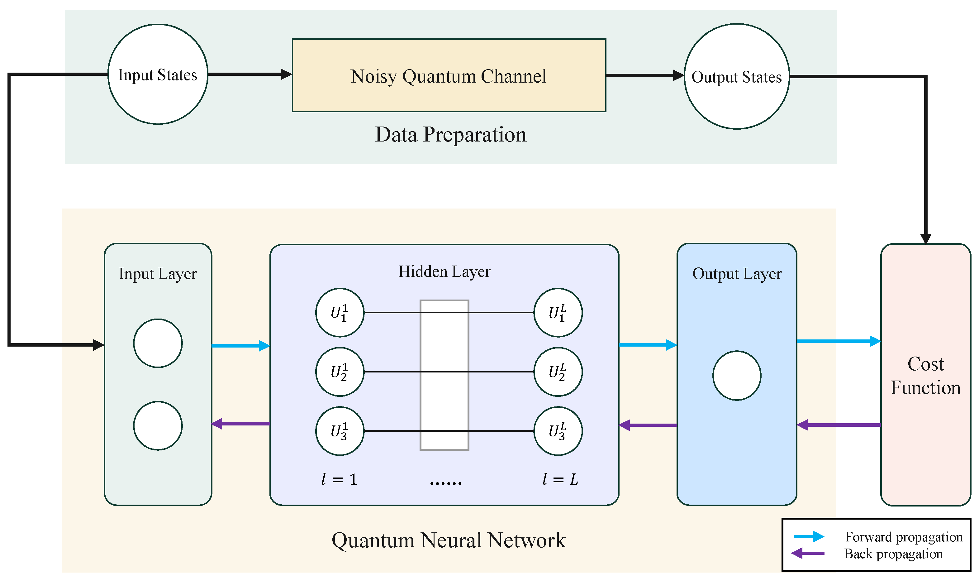
3.3. The Architecture of a Quantum Neural Network

The typical structure of a quantum neural network is similar to classical feed-forward neural networks, consisting of one input layer, one output layer and several hidden layers. For the hidden layers and the output layer, the output of the previous layer can be used as the input of the current layer. Figure 2 illustrates the architecture of a quantum neural network model, comprising two hidden layers, each containing three and four neurons, respectively.

Assume that the network has L hidden layers, the input of network is ${\rho }_{in}$ and the output is ${\rho }_{out}$, then the evolution of the quantum neural network can be expressed by the following equation:

$${\rho }_{out}\equiv t{r}_{in,hid}\left(\mathcal{U}{({\rho }_{in}\otimes |0\cdots 0\rangle }_{hid,out}\langle 0\cdots 0\left|\right){\mathcal{U}}^{†}\right),$$

(16)

where $\mathcal{U}\equiv U^{out}{U}^L{U}^{L-1}\cdots U^1$ represents the quantum circuit and $U^l$ denotes the U operator of the l-th layer which consists of neurons acting on the $l-1$-th and l-th layers.

Meanwhile, the depth of the network can be changed by changing the number of hidden layers. Furthermore, the width of the network can be changed by changing the number of neurons in each layer.

3.4. Training Process

The training process of the network can be understood as the process of tuning the value of each neuron in the network, and the goal is to find a set of suitable solutions to maximize the cost function. The cost function is defined as the calculation of the average fidelity between all outputs and the expected outputs of the network. The higher the cost value, the closer the output is to the expected value. This reveals the better performance of the training effect of the network. For pure quantum states, it can be described as

$$C=\frac{1}{N}\sum _{x=1}^N\langle {\varphi }_x^{out}|{\rho }_x^{out}|{\varphi }_x^{out}\rangle ,$$

(17)

where N represents the number of training data, ${\rho }_x^{out}$ is the output of the network and $|{\varphi }_x^{out}\rangle$ denotes the x-th output in the training data pair which is the expected output. When the output states of the training data are not pure, we use the fidelity for mixed states to describe it:

$$F(\rho ,\sigma ):={\left[tr\sqrt{{\rho }^{1/2}\sigma {\rho }^{1/2}}\right]}^2.$$

(18)

After obtaining the values of the cost function, updating the network parameters U is realized by backpropagation, and the network is then revolved with the new parameters U. The value of the cost function becomes larger after the update, i.e., the network fits the training data better. Backpropagation in quantum neural networks is referred to as the corresponding process in classical networks, and a detailed derivation can be found in [27].

4. Experiment Results

Here, in this part, we conduct experiments on 2D and 3D channels, and the results show that the quantum neural network can be generalized to higher dimensional channels.

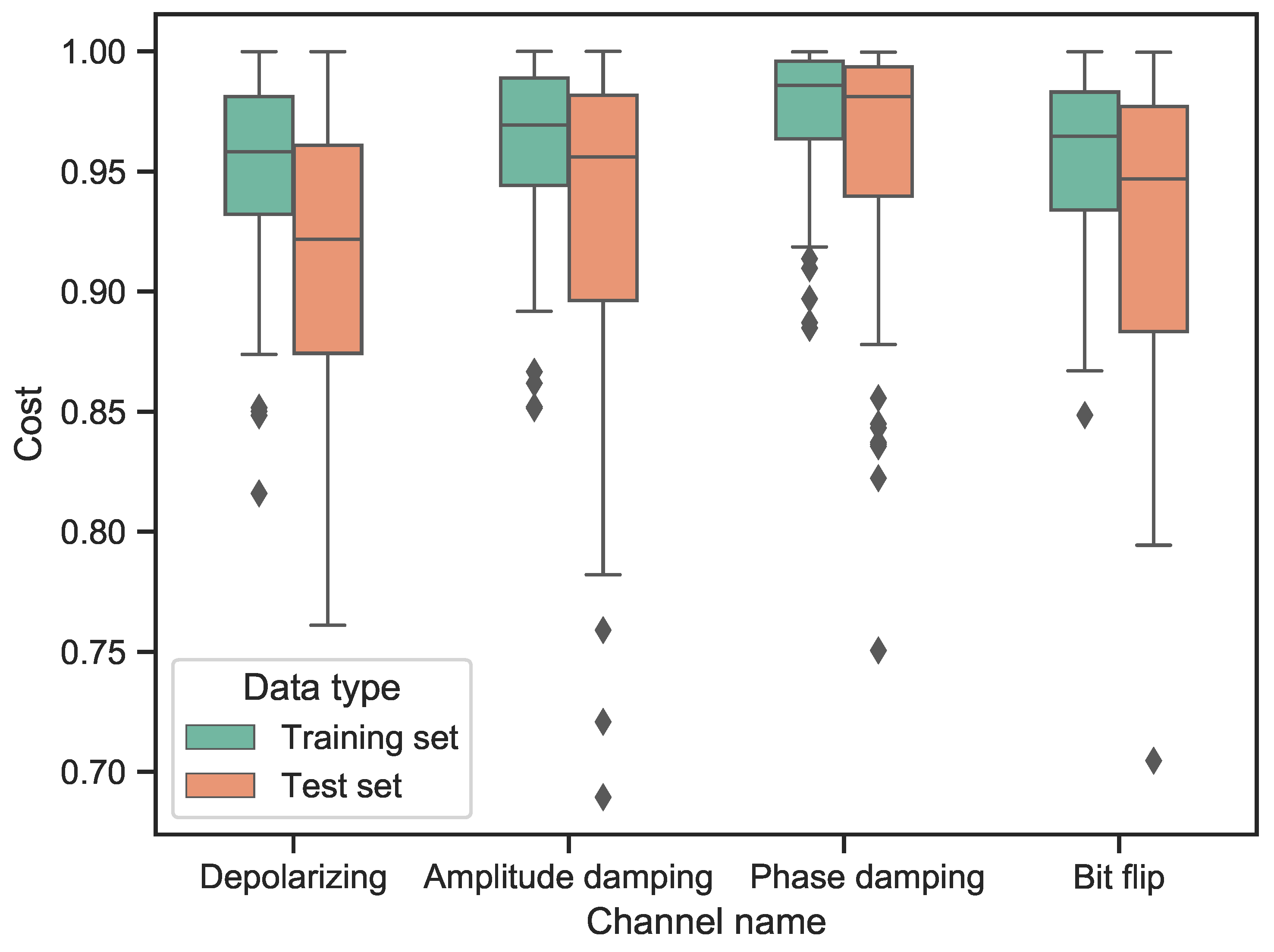
We use the proposed quantum neural network to train each of the four noisy quantum channels that are commonly used in the qubit transmission system 100 times, and the test set is used to evaluate the performance of the network. The structure of the network is [1, 2, 1], which means it has three layers including one input layer, one hidden layer and one output layer; the number of neurons each layer has is one, two and one. The number of data both in the training set and test set is 10 pairs. The results are shown in Figure 3.

The figure shows that the network is capable of generalizing the available information. As expected, the training costs are higher than the test costs. For different channels, the phase damping channel approaches the highest costs on both the training set and the test set, the amplitude damping channel performs better than the other two channels and the depolarizing channel obtains the lowest costs.

By analyzing the expressions of these four channels, we find that they have different levels of complexity. For example, the phase damping channel has a counter-diagonal value of 0, the amplitude damping channel has a constant value of 0, the value in the bit-flip channel is a real number and the depolarizing channel has an imaginary part. Combined with the experimental results, we believe that the neural network has a better training ability for the channels with simpler structures. Specifically, the channel with a simple structure has higher medians, upper bounds and lower bounds, indicating it has higher costs and more stable results. However, it has more outliers, which are caused by overfitting of the data.

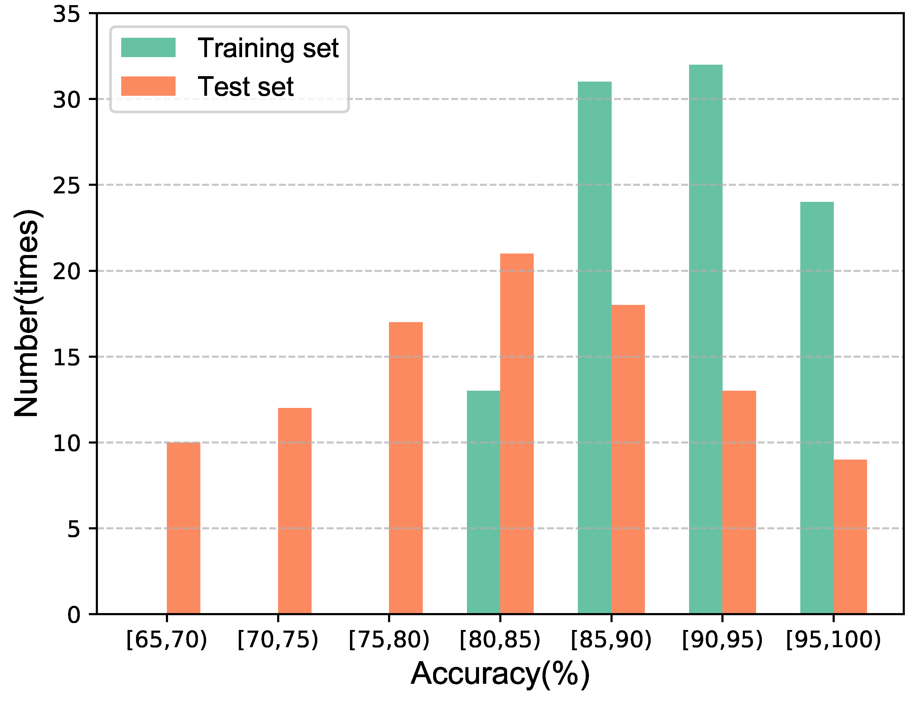
In the following, we use a quantum neural network with the structure of [1, 2, 1] to train a 3D noisy quantum channel 100 times, where the number of data both in the training set and test set is 10 pairs. We record the number of costs in each interval, and organize the results into a histogram, as shown in Figure 4.

The results show that the network could also be suitable for high-dimension channels. Although the cost is lower than that of lower dimensional channels, it also achieves an average of about 91% on the training set and 82.5% on the test set.

5. Methods to Improve the Performance of the Network

To improve the performance of the network, we conducted experiments and summarized all factors that may have effects on the network performance. Note that the conclusions we have drawn are generalized, the results shown below are representative and similar conclusions can be obtained even if different parameters are selected.

During training of a classical neural network, the performance of the model usually becomes better when the network structure becomes complex. We conducted related experiments on quantum neural networks but obtained different results. We trained networks with different architectures for the same amount of rounds, as shown in

Table 1. Performance of networks with different structures on a 2D channel.

Network Structure	[1, 1]	[1, 2, 1]	[1, 2, 2, 1]	[1, 2, 4, 2, 1]
Training cost	0.9598	0.9578	0.9542	0.9518
Test cost	0.9295	0.9286	0.9272	0.9259

and

Table 2. Performance of networks with different structures on a 3D channel.

Network Structure	[1, 1]	[1, 2, 1]	[1, 2, 2, 1]
Training cost	0.9496	0.9483	0.9317
Test cost	0.8825	0.9022	0.8958

. We find that as the network structure becomes more complex, the performance of the network becomes worse. This is caused by the speed of convergence; the simpler the structure of the network, the easier it is to train. As the training rounds increase, their cost values gets closer and the maximum cost value that can be achieved in the end is similar.

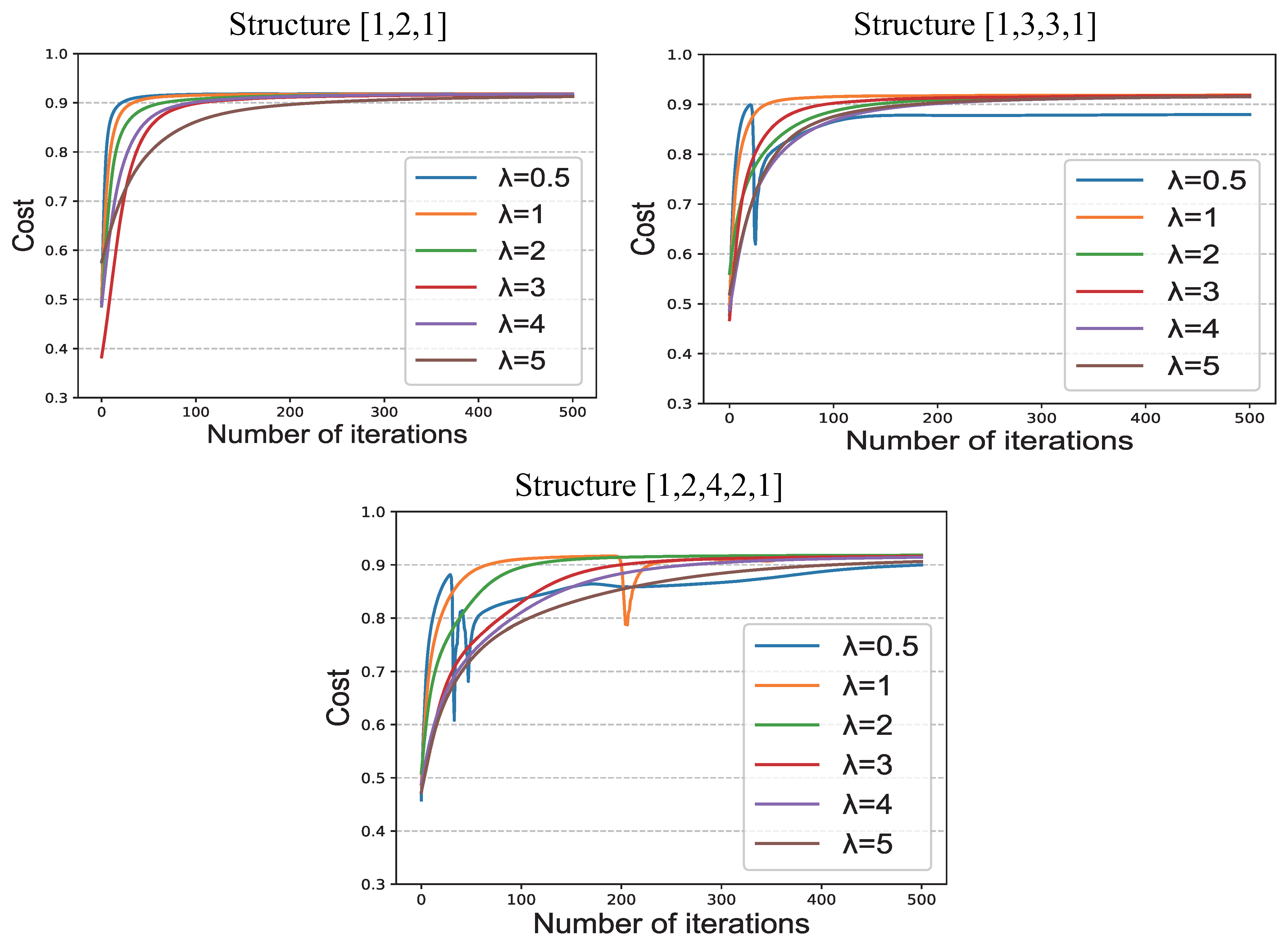
The hyperparameter $\lambda$ of the network is the reciprocal of learning rate $\eta$, that is to say, $\eta =1/\lambda$. We explored the effect of $\lambda$ on network performance, and the results are shown in Figure 5.

From the results in the figure, we can conclude that $\lambda$ affects the convergence rate. With a smaller value of $\lambda$, the faster the convergence rate. On the contrary, the convergence rate becomes slower with a larger value. However, this does not mean that a smaller value of $\lambda$ is better; for networks with more complex structures, too small a $\lambda$ will lead to abnormal convergence.

From the aspect of cost, we can see that as the number of iterations increases, the difference between the costs of different $\lambda$s becomes smaller.

Table 3. The relation between training rounds and cost.

Training Rounds	100	200	300	400	500	600	700	800	900	1000
Training cost	0.9485	0.9538	0.9550	0.9554	0.9557	0.9558	0.9559	0.9560	0.9561	0.9561
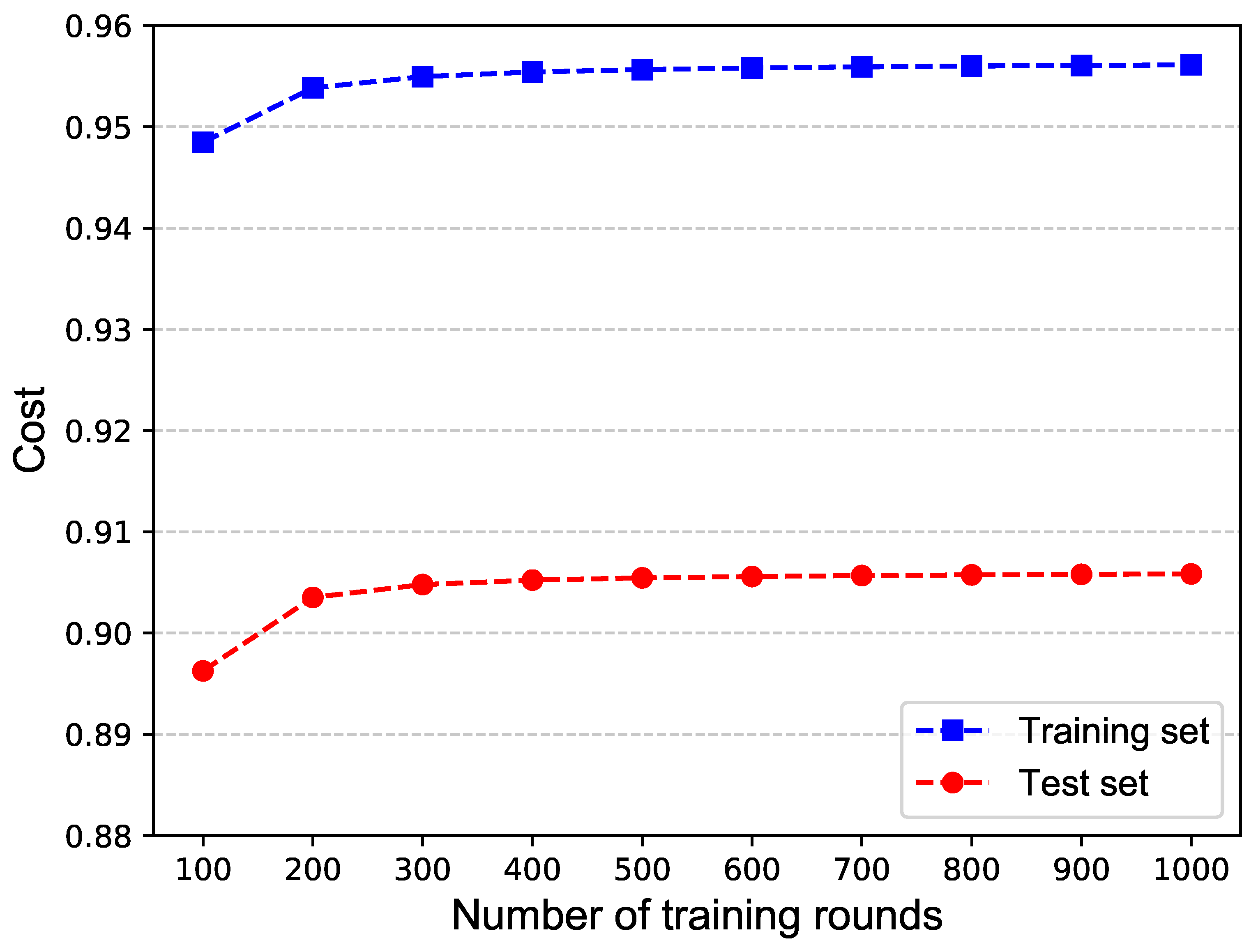
Test cost	0.8963	0.9035	0.9048	0.9052	0.9054	0.9056	0.9057	0.9057	0.9058	0.9058

shows the results of training a network for 1000 rounds. During the training process, the current optimal model is continuously updated and the results are output every 100 rounds. A visualization of the results is shown in Figure 6.

From the results, we can see that with the increase in the training rounds, the performance of the current optimal model becomes better both on the training set and on the test set.

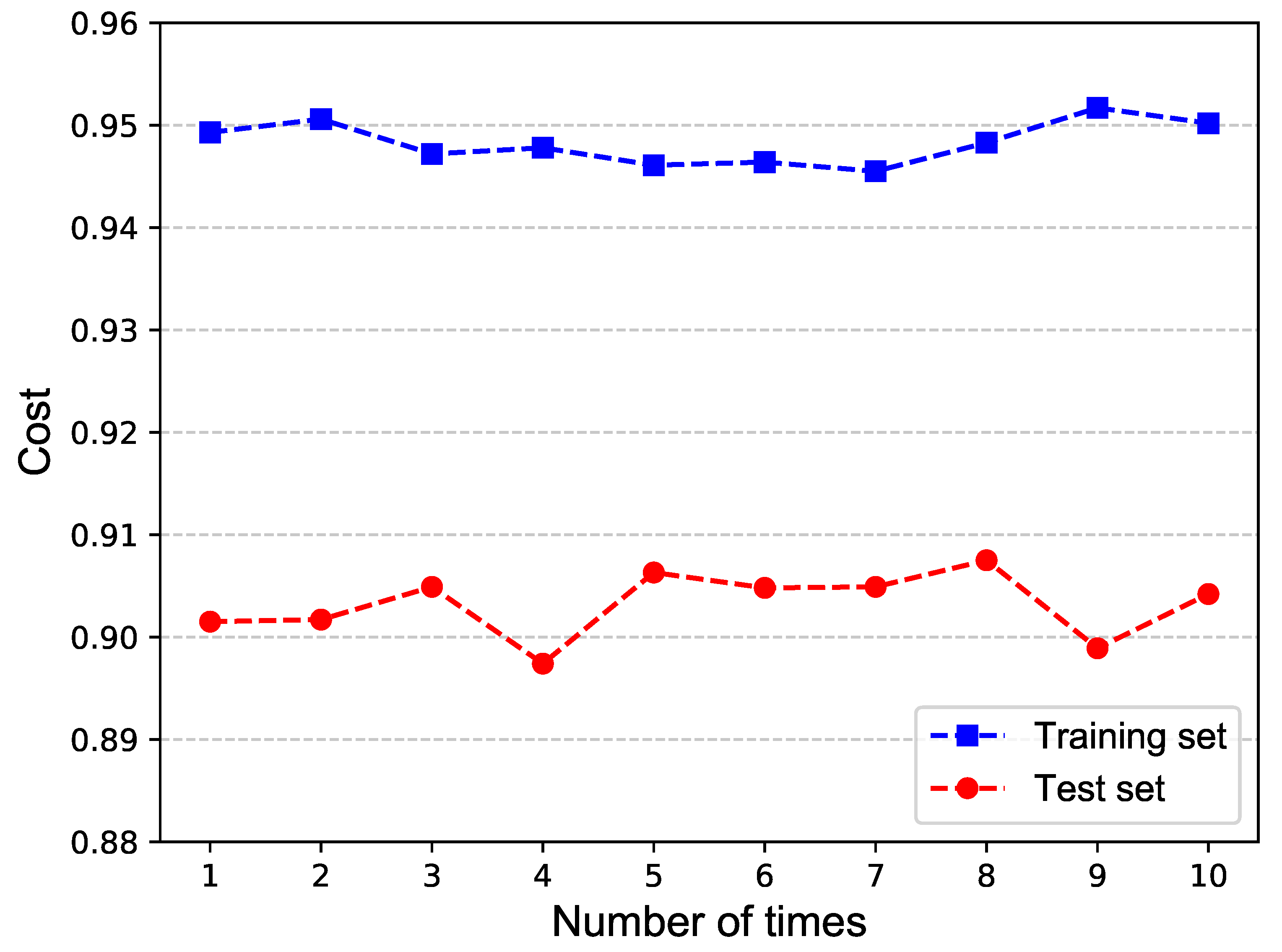
Moreover, we find there are differences in the results when training the same set of data several times. By analyzing the training process, we hypothesized that this is related to the random initialization of neurons represented by U-matrices. To verify the hypothesis, we performed ten experiments on one network; each experiment had the same parameters except for the U matrices.

The results are shown in

Table 4. The relation between random initialization and cost.

Number of Times	1	2	3	4	5	6	7	8	9	10
Training cost	0.9493	0.9506	0.9472	0.9478	0.9461	0.9464	0.9455	0.9483	0.9517	0.9502
Test cost	0.9015	0.9017	0.9049	0.8974	0.9063	0.9048	0.9049	0.9075	0.8989	0.9042

and Figure 7, from which we can learn that random initialization of U matrices does make a difference and this is uncontrollable.

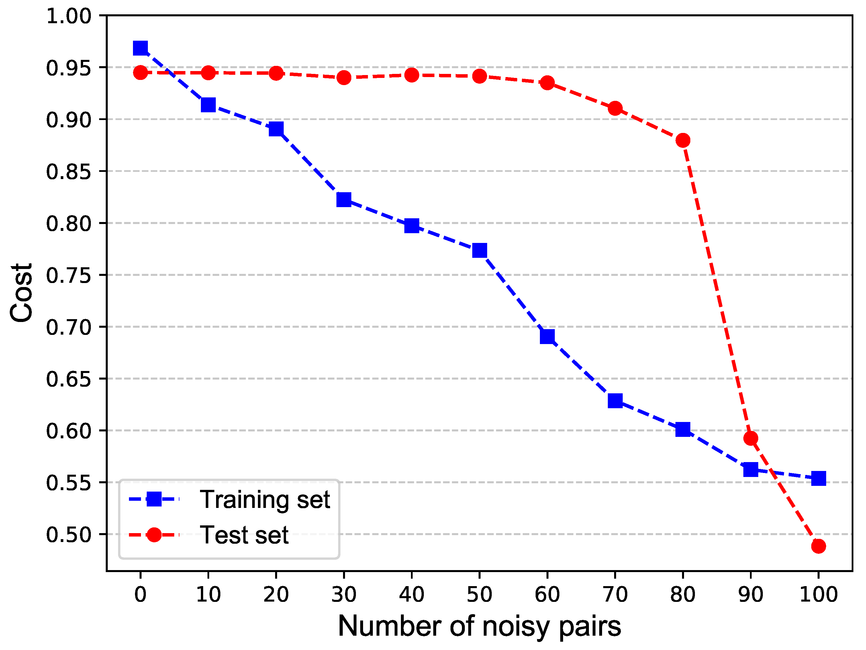
6. The Robustness of the Network

In this section, we focus on the property of robustness of the quantum neural network. We first trained a network with 100 training pairs and recorded the results, then the training pairs were replaced by noisy pairs. Replacement with noisy pairs was performed in units of 10, the noise pairs used here were randomly generated and there was no relationship between the input and output states in the pairs. The results are shown in

Table 5. The influence of the noisy pairs on cost.

Number of Noisy Pairs	0	10	20	30	40	50	60	70	80	90	100
Training cost	0.9686	0.9139	0.8907	0.8224	0.7974	0.7734	0.6904	0.6286	0.6010	0.5623	0.5538
Test cost	0.9449	0.9447	0.9443	0.9401	0.9426	0.9414	0.9351	0.9105	0.8796	0.5924	0.4884

and Figure 8.

From Figure 8, we can see that as the number of noisy pairs increases, both the training cost and the test cost decrease. When the number of noise pairs is less than 80, the value of the test cost is higher than 90%, which indicates the resistance of the network to noisy data, so we can conclude that the network is robust.

7. Discussion and Summary

In this paper, we use quantum neural networks to approximate the effect of a noisy quantum channel and conduct experiments on coherent noisy quantum channels. In the case of incoherent noisy quantum channels, the outputs are mixed states that can be described by density matrices. To model such channels, we can employ completely positive and trace-preserving (CPTP) maps and use incoherent quantum neural networks to approximate their effects. The cost function is then evaluated using the fidelity formula for mixed states.

In summary, we investigate methods for noisy quantum channel detection with a quantum neural network. The experiments conducted in this work have not yet been carried out on a quantum computer, but instead have been accomplished on a classical simulator. The current work mainly focuses on the study of noisy channels of different dimensions, determining how to improve the performance and testing the robustness of the quantum neural network.

According to the simulated results of 2D channels and 3D channels, we can conclude that using a quantum neural network may provide an efficient way to detect channel noise and it can be extended to higher dimensions. Then, we conducted experiments on all factors that may have impacts on network performance, including the network structure, the hyperparameters, the training rounds and random initialization. The results show that networks with simpler structures perform better when trained for the same amount of time. The hyperparameter $\lambda$ affects the training speed; a network with a smaller $\lambda$ has a higher training speed, but too small a $\lambda$ leads to errors for networks with complex structures. The network structure and hyperparameter $\lambda$ are set according to the problem at hand. The number of training rounds affects the cost both on the training set and the test set; it is beneficial to train as many times as possible. The random initialization of U matrices could lead to different results of the model and it is uncontrollable, but we can select the optimal model through multiple experiments to reduce its impact. Finally, we investigate the robustness of the network in noisy conditions.