1. Introduction
Since 2020, humanity has been in the mire of a global pandemic caused by a coronavirus named SARS-CoV-2 (Severe Acute Respiratory Syndrome CoronaVirus 2). The first cases of humans infected with coronavirus were officially reported in Wuhan, China, in December 2019. Since then, numerous investigations have been published regarding this pandemic [
1]. One of scientists’ biggest concerns is how this virus is transmitted between humans; as progress is made on this front, it seems clearer that the transmission of SARS-CoV-2 between humans is through the respiratory tract, either by close contact with an infected person, or through aerosols [
2].
That is why the measures adopted by most countries at this time are aimed at mitigating this means of transmission, such as wearing masks or social distancing [
3,
4]. In addition to the means of transmission, another determining factor of this virus is that it presents symptoms in the majority of infected people (up to
), which facilitates the spread of the virus, given that asymptomatic individuals can infect others with SARS-CoV-2. Furthermore, people with ordinary symptoms can progress to more serious symptoms, leading even to death [
5].
Even though several vaccines have been produced, controlling the spread of this virus appears impossible, as daily confirmed COVID-19 (novel COronaVirus Disease-2019) cases and deaths show [
6]. Governments around the world are seeking to find new and better vaccines [
7], while the virus continues to expand and mutate into different variants [
8]. How effective vaccines are against the different mutations of the virus has also been a subject of study [
9].
After being closed for a long period, schools are reopening, just as companies are asking their workers to return to work in person. In some companies, in-person work is essential, while in others it is dispensable, but it is more complex for schools to carry out their work remotely [
10]. Children need to be supervised by adults [
11], younger students need a follow-up from teachers [
12], and adolescents require face-to-face attention and assessment [
13]. Furthermore, university students require sophisticated training, which can only be achieved in person [
14].
This article aims to monitor the safety measures indicated to avoid the transmission of the virus in closed environments, using low-cost hardware resources so that the system can be acquired by any company (store, bar, cultural center, hypermarket, etc.), university, or school. A deep-learning-based solution, which is a continuation of a previous work of the author [
15], is proposed for the detection of people, as well as for monitoring their social distancing. It is also essential to detect possible crowds. For this purpose, a basic interior furniture (e.g., tables) detection system was implemented, since people seated around the same table, for example, in a bar, would not be considered a crowd up to a certain limit, as established by the health authorities.
In any of the above-described situations, the alert system is in charge of sending a notification to the owner of the site via SMS and e-mail. To test the behavior of the system, numerous experiments were conducted in a real environment, specifically at the entrance and exit of classes at Rey Juan Carlos University. The hardware platform used for this was based on the Raspberry Pi 4 board as the central processing unit, to which a pair of RGB cameras—model PiCamera—were incorporated to capture the color images of the environment, and an Intel Neural Stick to lighten the execution of the deep learning algorithms. The results (described in
Section 5) show that the system performs plausibly, with a very fast response in real-time detection of the situations described.
2. Related Works
Previous works conducted with the same purpose of maintaining social distancing using a control system are presented in this section. All of these were motivated by the pandemic generated by the SARS-CoV-2 virus. In [
16], an effective social distance monitoring solution in low-light environments is described. Low-light environments can be a problem in the spread of disease because of people gathering together at night. This is especially critical in summer when temperatures reach a peak and people go out of their homes with their families at night to enjoy the cooler air. A deep-learning-based solution is proposed for the above-stated problem. It uses YOLO (You Only Look Once) v4 model for real-time object detection and the social distance measuring approach is introduced with a single motionless ToF (Time of Flight) camera.
In [
17], the YOLO v3 object recognition paradigm to identify humans in video sequences is also used, but the authors add a transfer learning methodology to increase the accuracy of the model. In this way, the detection algorithm uses a pre-trained algorithm that is connected to an extra-trained layer using an overhead human data set. The detection model identifies people by means of detected bounding box information. The pairwise distances between the centroids of the detected bounding boxes are determined using the Euclidean distance. To estimate social distance violations between individuals, an approximation of the physical distance in pixels is used. A violation threshold is established to evaluate whether or not the distance value breaches the minimum social distance threshold.
In [
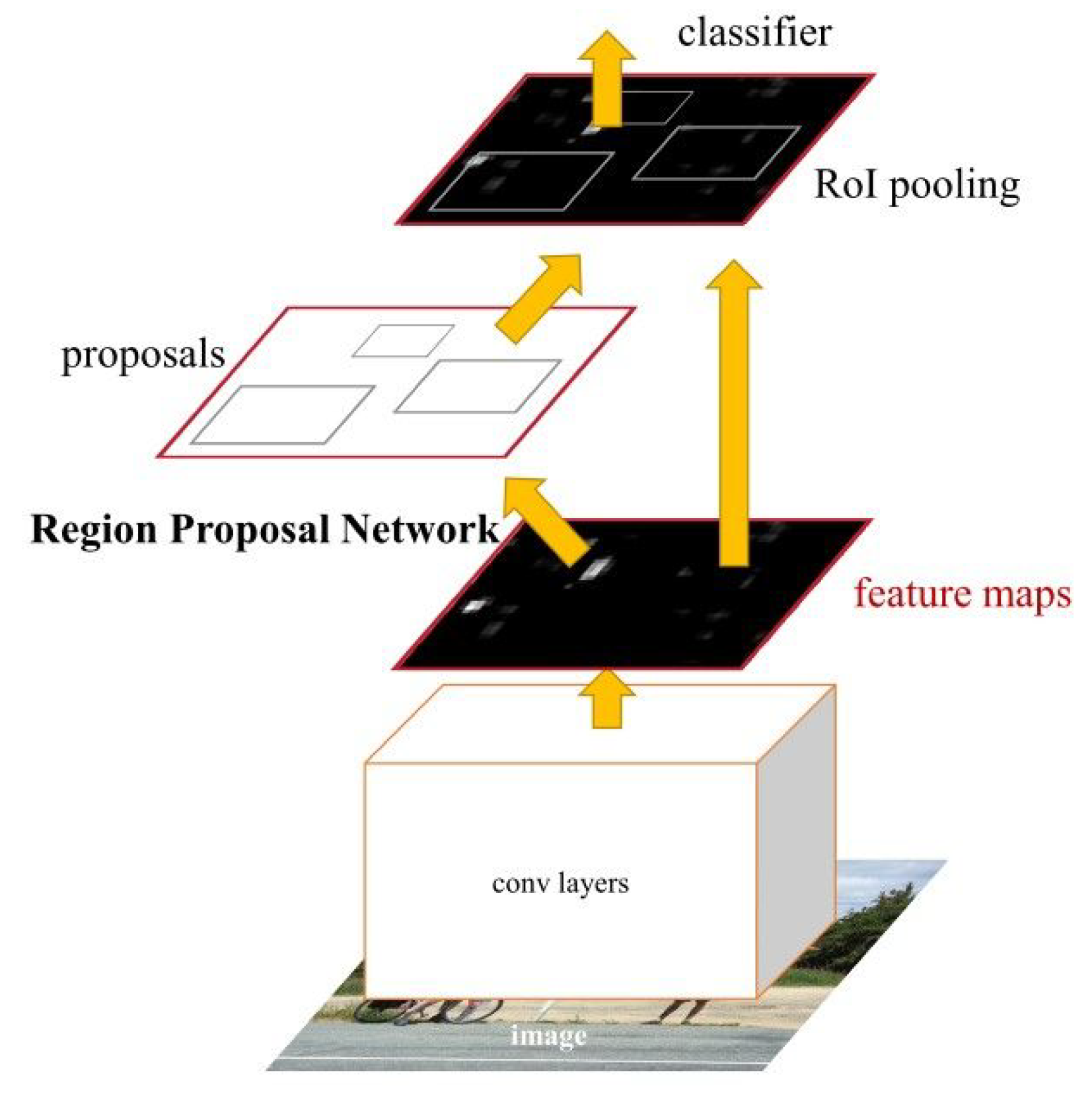
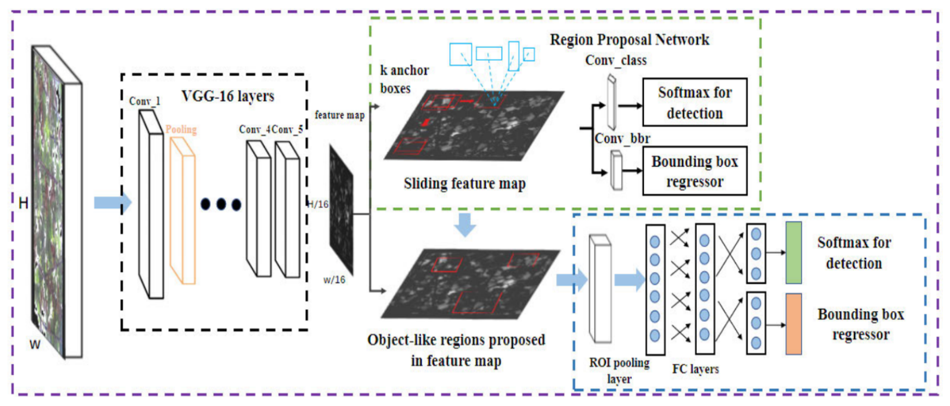
18], an improvement was introduced: the use of Faster R-CNN (instead of Fast R-CNN) for human detection in the images. The Fast R-CNN model consists of a single-stage, compared to the three stages in R-CNN. It was developed to improve the speed and accuracy of object detection in images. However, the architecture of Faster R-CNN—shown in
Figure 1—consists of two modules: the Region Proposal Network (RPN) and the algorithm of Fast R-CNN, for detecting objects in the proposed regions. The Fast R-CNN algorithm consists of the following key steps:
- 1.
Region Proposal: Initially, a set of potential object regions, known as region proposals, are generated using the selective search or another similar method. These region proposals are areas in the image that are likely to contain objects.
- 2.
CNN Feature Extraction: A convolutional neural network (CNN) is employed to extract features from the entire input image. This CNN is typically pre-trained on a large dataset (such as ImageNet) and can capture useful visual representations.
- 3.
Region of Interest (RoI) Pooling: The extracted CNN features and the region proposals are used to create fixed-size feature maps for each region proposal. RoI pooling is applied to warp these feature maps into a fixed spatial extent, allowing subsequent layers to process them.
- 4.
Classification and Localization: The RoI-pooled features are fed into fully connected layers that perform both object classification and bounding box regression. The classification network predicts the probability of each region proposal belonging to different object classes, while the regression network estimates the refined coordinates of the object’s bounding box.
- 5.
Non-Maximum Suppression: After classification and regression, the algorithm applies non-maximum suppression to remove redundant and overlapping bounding box predictions. This step ensures that each object is represented by a single bounding box with the highest confidence score.
Fast R-CNN combines region proposal generation, feature extraction, and object classification/regression into a single end-to-end network, which makes it faster and more efficient compared to its predecessors. By sharing the computation of the CNN features among different region proposals, it significantly speeds up the detection process. In addition, Faster R-CNN typically outperforms Mask R-CNN, which was proposed in [
19], in terms of bounding box detection because it has a simpler architecture and focuses solely on object localization. Mask R-CNN, on the other hand, extends Faster R-CNN by adding a branch for pixel-level segmentation. This additional complexity in Mask R-CNN can lead to decreased performance in bounding box detection compared to Faster R-CNN.
In [
20], an active surveillance system to slow the spread of COVID-19 by warning individuals in a region of interest is proposed. These authors’ contribution is twofold. First, they present a vision-based real-time system that can detect social distance violations and send non-intrusive audio-visual cues using state-of-the-art deep-learning models. Second, they define a novel critical social density value and show that the risk of social distance violation occurrence can be held near zero if the pedestrian density is kept under this value.
In [
21], a two-component model is proposed. The first component was designed for the feature extraction process based on the ResNet-50 deep transfer learning model, while the second component was designed for the detection of medical face masks based on YOLO v2. Two medical face mask datasets were combined into one for investigation in this research. To improve the object detection process, Intersection over Unit (IoU) was used to estimate the best number of anchor boxes. The results obtained concluded that the Adam optimizer presented in [
22] achieved the highest average precision percentage of
as a detector, compared to the Stochastic Gradient Descent with Momentum (SGDM) optimizer technique, which was presented in [
23].
Several research studies have been conducted to provide a solution to maintaining an effective social distance as discussed above. However, none of the studies focused on providing a real low-cost solution accessible to everyone; that is, using a hardware platform that is computationally adequate to support the complex detection algorithms used, but sufficiently economical to be affordable for any company, small or large, and which can be acquired anywhere in the world. The present article addresses this deficiency. A sophisticated and robust detection software system based on deep learning techniques was developed, focusing the implementation on its efficiency so that it can be run under the demands of a system that operates in real-time on a low-cost hardware platform.
3. Method
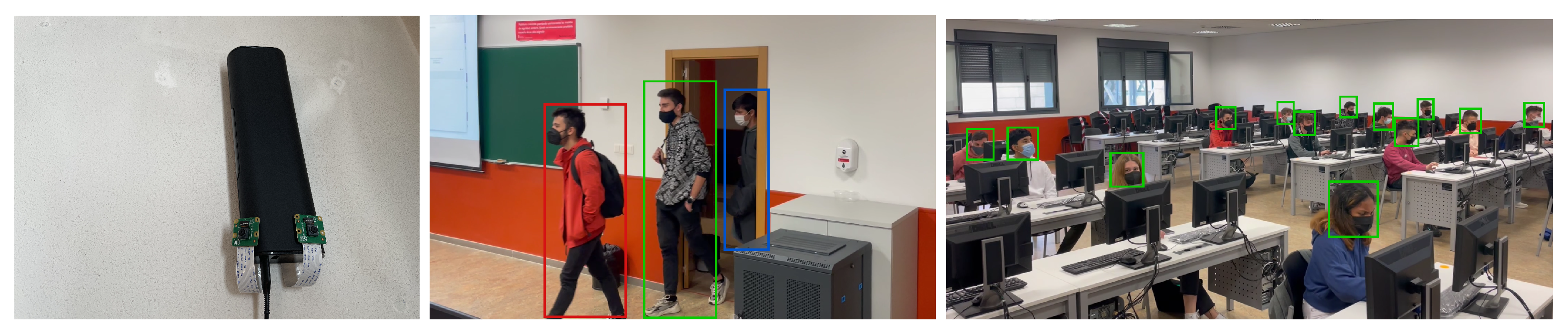
The method proposed in this work consists of using two RGB cameras (
Figure 2(left)), specifically, two PiCamera model cameras, to detect people within the frame of the image, and with this, calculate the interpersonal distance. One camera focuses on the entrance door (
Figure 2(middle)), and the other on the area of the room where the people entering sit (
Figure 2(right)). If the system detects that at any time the established social distance is not being respected, it notifies the person in charge of the room via SMS/e-mail.
3.1. Object Detection
First, a Faster R-CNN object detection network was used, which was adapted to detect a new set of objects, with their orientation and dimension. To achieve this goal, the last layers of the architecture were modified, because they determine the number of classes to work with and how to do them.
The result of a Faster R-CNN is a bounding box that locates the object detected in the image, but lacks information about its absolute position in the real world; new layers are needed to estimate such a position. The implementation used in this work is based on the development presented in [
24]. These authors extended the Faster R-CNN architecture with new layers to support the bounding cube concept. The bounding cube could be defined as the smallest rectangular parallelepiped that contains the object. It includes the orientation and dimensions of the object.
The bounding cube is determined by its center , dimensions , and orientation , where represents the special orthogonal group in three dimensions. The special orthogonal group consists of all matrices that are both orthogonal (their transpose is equal to their inverse) and have a determinant of 1. In other words, the elements of are rotation matrices that preserve the orientation of a three-dimensional object.
Given the pose of the object in the camera coordinate frame and the intrinsic matrix K, the projection of a 3D point in homogeneous coordinates, in the coordinate frame of the object in the image is .
Assuming that the origin of the object’s coordinate system coincides with the center of the bounding cube and dimensions
D are known, the vertices of the bounding cube are as described in Equations (
1)–(8).
The restriction that the bounding cube is enclosed by the bounding box means that each side of the 2D detection has to coincide with the projection of—at least—one of the vertices of the bounding cube. If the bounding box is given by the lower left vertices (
) and upper right (
), and it is also known that, for example, the 3D point
projected falls on the left side of the detection, Equation (
9) can then be posed.
Equation (
9) indicates the
component of the perspective projection. It is a formulation to calculate the x-coordinate of the lower-left vertex (
) of the bounding box based on the projection of a 3D point (
) onto the image plane. The equation incorporates the camera intrinsic matrix
K, the rotation matrix
R, the translation vector
t, and the 3D coordinates of the point (
,
,
). The homogeneous coordinate mechanism was already addressed profusely in previous works by the author [
25,
26].
Analogous Equations (
10)–(12) can be set for
if we know the correspondence of which vertex of the bounding cube is projected to which side of the bounding box.
Each of Equations (
10)–(12) indicates each component of the perspective projection and
according to which vertex corresponds. In total, these four restrictions are sufficient to determine
t, if
K,
R and
d are known.
K is a constant that is known to be the intrinsic calibration matrix of the camera [
25,
26], while
R and
d will be parameters estimated by the neuronal network as explained below in
Section 3.2.
3.2. Calculating R and d
A Faster R-CNN architecture applies the RoI (Region of Interest) pooling layer to propagate forward the feature maps of each object region. This means that, for any regression or classification layer, the data obtained from the subregion image being processed at that time will be applied. In other words, the Faster R-CNN output for a sub-region is invariant with respect to its translation in the image. For this reason, it was decided not to directly estimate orientation of the object with respect to the camera, since—in the upper layers—the Faster R-CNN loses the information about where the object is in the image. Instead, the network estimates a local angle that is invariant to the translation of the object in the image.
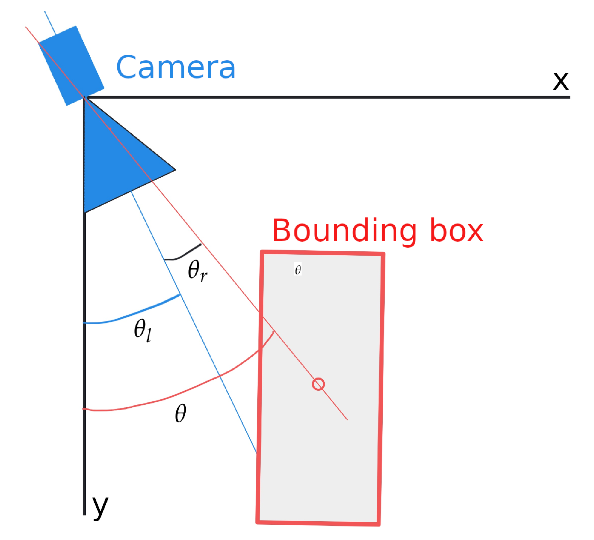
Rotation matrix
is only parameterized by a rotation with respect to the vertical axis with angle
. This angle can be decomposed as shown in Equation (
13), where
is the local angle of rotation that the object forms with the ray that goes from the camera towards the center of the bounding box and
the angle that this ray forms with the camera (
Figure 3).
Instead of predicting angle
directly, the network regresses on the local angle of rotation
, and angle
is obtained by combining the angles
and
according to Equation (
13); namely, the angle
can be calculated from the location of the bounding box in.
To estimate the parameter with the network, the same approach as Faster R-CNN is used to conduct regression on the bounding boxes, which means discretizing the solution space in m classes, each associated with an angular interval. For each of these classes, the network estimates its probability that belongs to it and the residual angle that remains to be applied to the central angle of that class to obtain the local rotation. In practice, the value estimated is that of the sine and cosine of this residual angle, with the network having three outputs for each angular class i: .
The cost function is defined as shown in Equation (
14), where the confidence
is the softmax cost of the trusts of each angular class,
is the cost function that attempts to minimize the difference between the estimated angle and the ground-truth for each of the intervals to which the angle of the ground-truth belongs, and
w represents a weight or coefficient that determines the relative importance of the two terms in the cost function.
Minimizing this difference is equivalent to maximizing its cosine, so that Equation (
15) can be posed, where
is the angle of the ground-truth,
is the number of intervals that contain
,
is the central angle to the interval
i, and
is the residual angle to be applied to the center of the interval
i.
To estimate
, a continuous approach is used to do a regression without discretizing the space of solutions. In most classes, the distribution of their possible dimensions has low variance, so we proceeded with the traditional technique of regression on the residual with respect to the average of the training values for each parameter, with a cost function as shown in Equation (
16), where
is the ground-truth of the dimensions,
is the average of dimensions for objects of a certain category, and
is the residual value with respect to the average predicted by the network. The total cost function is defined in Equation (
17), where
represents (as its analog
w in Equation (
15)) the weight of the cost function.
3.3. Vertex to Side Correspondence
Using the network estimated of the rotation
and dimensions
, the translation
can be estimated from Equations (
9)–(12), and be calculated for each side assignment from bounding box to a vertex of the bounding cube. After trying all the combinations, the
t that minimizes the reprojection error of the bounding box is the
t to be chosen.
In the beginning, each side can correspond to a vertex, resulting in configurations. To reduce the computation time, the camera is assumed to be parallel to the ground, and the object is assumed to be always stationary, rotated on its vertical axis, but without other inclinations, such as most everyday objects (e.g., furniture).
As the object is only rotated about the Z axis, is determined by some of the lower vertices and by one of the superiors. Furthermore, it can be assumed that both and are determined by two of the lower vertices because all the points on one side vertical are projected at the same x image coordinate). Therefore, it is only necessary to evaluate combinations to obtain the one that minimizes the reprojection error of the bounding box.
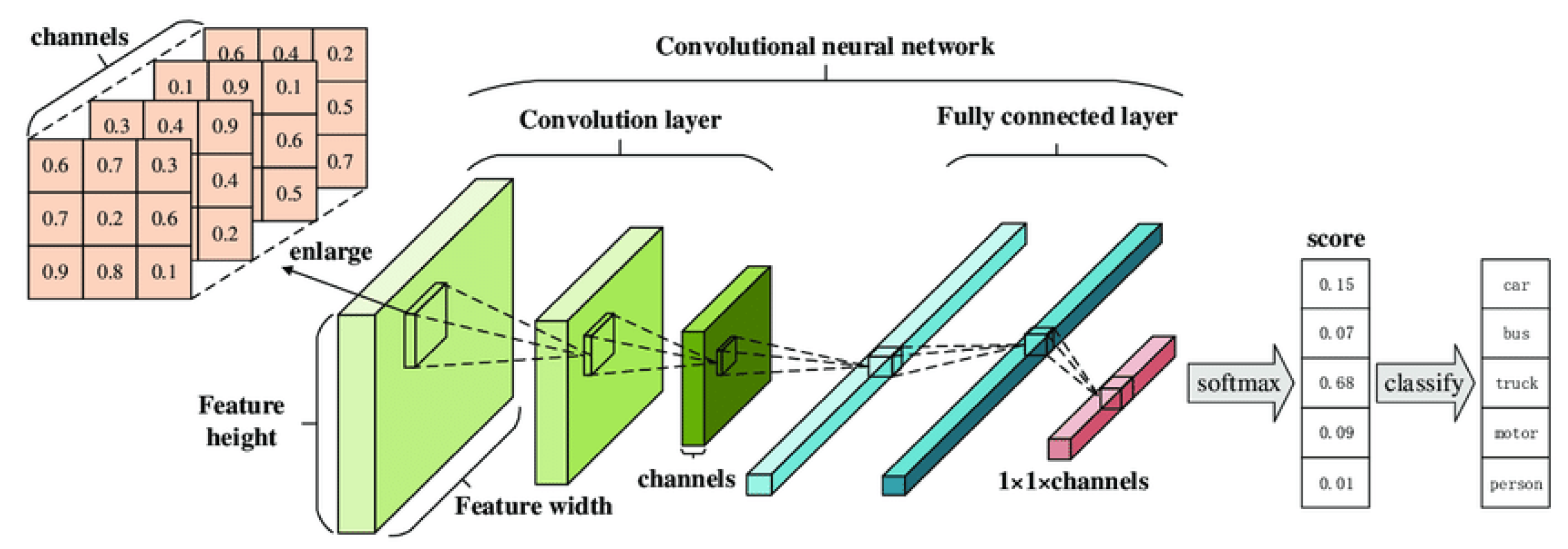
4. Architecture
The general architecture of the proposed system follows the model of a Faster R-CNN, which is an improved version of a Convolutional Neural Network (CNN). The traditional CNN structure is shown in
Figure 4 [
27], and the improved Faster R-CNN architecture is shown in
Figure 5 [
28].
4.1. Trained Neural Network
The first requirement for the proposed system to work is to have a trained neural network. To accomplish this, different photographs were taken of real scenarios corresponding to classrooms and laboratories at Rey Juan Carlos University (
Figure 6). These images include bounding boxes of the objects present, such as students’ desks, along with their positions relative to the origin of coordinates in the classroom.
The origin of the coordinates is in the center of the classroom, which was previously measured manually. A mark is made on the ground at the center, and the camera is calibrated accordingly to ensure its orientation is precisely towards that point. The camera is always located in the same position: next to the entrance door, on the left, checking that the different points of view of the objects are as uniform as possible.
In this way, the necessary ground-truth is obtained for each object in the image, its class, bounding box, orientation, and dimensions. Since the camera position is always at the front of the classroom, the desk models are consistently aligned; that is, the Y axis of all the desks always points towards the backrest.
4.2. Software Platform
The modified Faster R-CNN architecture was implemented in
Pycaffe, and so the Stochastic Gradient Descent (SGD) optimizer implemented in
Caffe [
29] was used, with the initial weights of the Faster R-CNN network already trained in the COCO (Common Objects in Context) dataset [
30].
The training scheme consisted of a first preliminary training with COCO real images (
https://cocodataset.org/#download (accessed on 13 February 2023)) in the classes in common with those used in this work, followed by training with images of real classrooms at Rey Juan Carlos University, to finish with a longer training of the layers dedicated to the prediction of the pose with the system’s dataset.
For each image sent to the object detector, the only objects considered are those that should be observed, projecting their bounding cubes onto the image. Of these objects, those that were detected in the image are called inliers, and those that were not, outliers. Throughout the execution for each object on the map, its positive detections (
, in which it was an inlier) and its non-detections (
, in which it was an outlier) are counted separately. Based on the difference of these metrics, a
level of confidence is established in the objects (
o) on which three thresholds are defined as described in Equation (
18) (T_L is TRUST_LEVEL):
The precursor to this level of trust idea was already described in the author’s work in [
31] under the concept of
life dynamics.
For the objects finally considered as trusted, their rotation matrix
R and translation
t are obtained with respect to the camera, starting from the network output. Rotation matrix
R is determined from the orientation angle with respect to the camera, obtained from the sum of the ray angle of the bounding box and the local angle. If Equation (
9) is developed, it is obtained that, for a given point
, the projection onto the image plane in homogeneous coordinates is obtained according to Equation (
20).
Thus, if
determine the vertices
, their projections onto the image plane in homogeneous coordinates are obtained in Equations (
21)–(24).
Finally,
can be obtained, based on the width (
w) (Equation (
25)) or height (
h) of the bounding box, and then,
and
are obtained.
5. Experiments
This section describes the experiments conducted. The parameters used in each Faster R-CNN test and the results obtained in each case are detailed. Subsequently, an optimal model was chosen for each method. The model with the most favorable results will be used in the candidate generation stage to obtain the prediction of a person in the picture. Finally, a general discussion is presented based on the results obtained during experimentation.
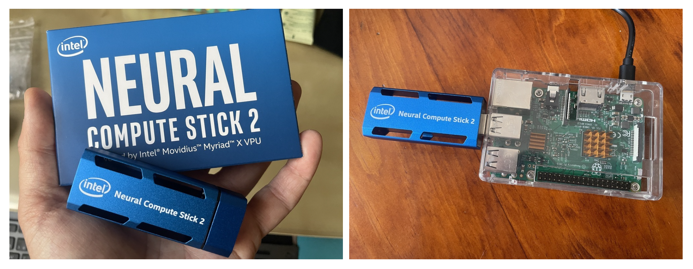
All experiments were carried out over a Raspberry Pi 4 as a main board, which incorporates the chipset Broadcom BCM2711 with a quad-core ARM (v8) Cortex-A72 64-bit processor at 1.5 GHz, and 8GB LPDDR4-3200 SDRAM. An Intel Neural Stick (
Figure 7(left)) was added to the main board (
Figure 7(right)) to accelerate the deep learning inference.
As described in Section, a pair of RGB PiCameras were used (
Figure 2): one to obtain images of the entrance door and another to capture images of the room. The reason for using this type of camera on this hardware platform is that they are directly connected through the CSI port of the board, providing better performance compared to a USB camera, as was described in [
26].
5.1. Neural Network Parameters
The parameters studied to obtain the different Faster R-CNN models and implement them on the network algorithm are as follows:
: width of the trained image.
: height of the trained image.
: number of channels (RGB).
: color depth; number of bits that are needed to represent a color.
: number of feature maps of the first convolution layer. The values 8, 16 and 32 were tested, in concordance with the second layer.
: number of feature maps of the second convolution layer. The values 16, 32, and 64 were tested, in concordance with the first layer. Therefore, the pairs are as follows: 8–16, 16–32, and 32–64.
: number of hidden fully connected units. The values 128, 256, 512, and 1024 were tested.
: Number of labels or classes. Since it is a question of classifying between person or non-person, its value is 2.
: number of training examples in a single batch (batch).
: an epoch occurs when an integer dataset is passed back and forth through the neural network only once. Since the training of the network is an iterative process, this process must occur repeatedly.
: number of convolution layers. It starts with two and a model with four layers is trained.
: the filter pass in the convolution operation.
: padding to be added after convolution, which allows the output image to be the same size as the input image.
: as was described in
Section 4.2, the Stochastic Gradient Descent (SGD) optimizer, implemented in
Caffe [
29], is used.
: the early stopping regularization technique is used to reduce overfitting.
Table 1 shows the various training models and their associated parameters. For the first 10 models, the feature maps are modified while keeping the convolution filters fixed. Starting from the 11th model, the best-valued parameters are fixed, and the combination of convolution filter and max-pooling filter is varied, which remains consistent across both layers. Lastly, the 16th model incorporates the two optimal parameters from the previous groups and includes two additional convolution layers.
5.2. Results of Training and Testing Person Detection
The ML metrics used in this work are the following:
Precision: it quantifies the proportion of true positives (correctly predicted positive instances) out of the total instances predicted as positive. It focuses on the correctness of positive predictions and is useful when the cost of false positives is high.
Recall (Sensitivity or True Positive Rate): it measures the proportion of true positives identified correctly out of the total actual positive instances. It emphasizes the completeness of positive predictions and is valuable when the cost of false negatives is high.
F1 Score: it combines precision and recall into a single metric by taking their harmonic mean. It provides a balanced evaluation of a model’s performance, considering both precision and recall.
Accuracy: it measures the proportion of correctly classified instances out of the total number of instances. It is a widely used metric, especially for balanced datasets. However, it can be misleading when dealing with imbalanced datasets.
where:
TP: True Positives
where:
The evaluation metrics used are defined as described in Equations (
28) and (
29). It can be observed that the
could be considered a more precise measure than the
since it incorporates false negatives in its value, which can distort the actual result. Additionally, the
is considered a reliable measure when dealing with uneven class distribution.
where:
TN: True Negatives
Below are the comparative tables with the person detection results obtained when training the different models explained in
Section 5.1, both in the train (
Table 2) and test (
Table 3) sets.
Analyzing the training results of Faster R-CNN models 1 to 10, it can be observed that generally higher accuracy is obtained with a higher number of hidden units. The models with demonstrate better results in the training set; however, they also consume more resources. On the other hand, lower and medium values yield similar but lower results.
On the other hand, the training results from Faster R-CNN models 11 to 15, in which the number of feature maps () of the first and second convolution layers is a constant value, show that increasing the value of the convolution filters increases the accuracy value. Increasing the value of max-pool from 2 to 4 decreases the result.
It can be concluded that in the training set, increasing the number of features generally leads to a decrease in error. Precision improves with an increase in the number of feature maps and hidden units. However, increasing these parameters also results in longer training times and a higher demand for computational resources.
Table 2 shows the results of the training in the test set. These results are those that were considered when choosing the optimal Faster R-CNN for the system detection process. It can be observed that the best results are yielded by adding two more convolution layers (model 16) and combining mid-term values of the rest of the parameters (model 7).
It can also be observed that the results in the test set are slightly lower than those in the training set. Once again, in most cases, higher numbers of features lead to better results. Additionally, it can be seen that increasing the max-pooling value from model 11 to 15 results in lower performance.
5.3. Results of Training and Testing Object Orientation
To evaluate the orientation predictions, the real image datasets were also used, as well as the synthetic image dataset. The 3D object detection and orientation estimation was evaluated using the Average Orientation Similarity (AOS) measure, a concept introduced in [
32] and which is defined as shown in Equation (
30).
where:
r: recall (described in Equation (
28))
s: orientation similarity ()
In addition,
s at recall
r is a normalized (
) variant of the cosine similarity defined as shown in Equation (
31). In other words, the AOS measure considers the precision of the detections weighted by the similarity of the cosine of the angles.
where:
D(r): set of all object detections at recall rate r
: difference in angle between estimated and ground truth orientation of detection i
: used to penalize multiple detections which explain a single object (Equation (
32))
Table 4 shows a comparison of the maximum values of Average Precision (AP), Average Orientation Similarity (AOS), and Orientation Score (OS) obtained for the different training iterations of the RPN detection layer with synthetic data. In all these cases, the orientation layers were trained for 200 k iterations.
6. Conclusions
This work presents a visual system that enables users to control safety measures aimed at preventing the transmission of viruses in enclosed environments, utilizing cost-effective hardware. The solution relies on deep learning for the detection of people, as well as basic furniture such as tables, and for monitoring the social distancing maintained between individuals.
To implement the system, a feature-based stereo vision was integrated with a modified and extended Faster R-CNN network, specifically tailored for detecting a new set of objects along with their orientation and dimensions. To accomplish this, the final layers of the architecture were modified to determine the number of classes and their handling.
Additionally, new layers were incorporated into the Faster R-CNN to estimate the absolute position of the detected objects in the image. This addition was necessary as the original Faster R-CNN output only provided bounding boxes without information about their real-world position. The proposed architecture includes these new layers to support the concept of a bounding cube, encompassing the object along with its orientation and dimensions.
The performance of the object detector was evaluated on both real and synthetic image datasets, employing various training schemes. Furthermore, a dataset consisting of six sequences captured in office environments was developed to comprehensively test the entire system.
7. Discussion
The results of this study highlight the effectiveness of the control system for indoor safety measures based on the Faster R-CNN architecture. The system successfully detects and recognizes potential safety hazards in real-time, including capacity control, social distancing, and mask use. By utilizing deep learning techniques, the system promptly identifies these situations that require control and promptly notifies the responsible personnel if any violations occur.
The evaluation of the proposed system was conducted in a real teaching environment at Rey Juan Carlos University, utilizing Raspberry Pi 4 as the hardware platform, along with the Intel Neural Stick board and a pair of PiCamera RGB cameras for image capture. The Faster R-CNN architecture was employed to detect and classify objects within the images. To assess its performance, a dataset of indoor images was collected and annotated for object detection and classification. Precision, recall, and F1 score were utilized as evaluation metrics.
The results demonstrate that the proposed system achieves a high level of accuracy in detecting and classifying potential safety hazards in indoor environments. This indicates its reliability and effectiveness in identifying safety violations in real-time. Moreover, the system’s software infrastructure is efficiently implemented and designed to be compatible with low-cost hardware platforms, making it affordable for companies of any size or revenue. Furthermore, the potential for integration into existing safety systems in various indoor environments, such as hospitals, warehouses, and factories, provides real-time monitoring and alerts for safety hazards.
As for future work, the focus will be on improving the system’s robustness and scalability to larger indoor environments with more complex safety hazards. This would enhance its applicability and allow for its seamless integration into a wider range of settings. Overall, the results of this study demonstrate the efficacy of the proposed control system, highlighting its potential to contribute to safer indoor environments and facilitate proactive safety management.


