DVL Model Prediction Based on Fuzzy Multi-Output Least Squares Support Vector Machine in SINS/DVL

Abstract

For an underwater Strapdown Inertial Navigation System/Doppler velocity log (SINS/DVL) integrated navigation system, the short-term failure of DVL may lead to the loss of reliable external velocity information from DVL, which will cause the SINS errors to accumulate. To circumvent this problem, this paper proposes a velocity predictor based on fuzzy multi-output least squares support vector machine (FMLS-SVM) to predict DVL measurements when DVL malfunctions occur. Firstly, the single-output least squares support vector machine (LS-SVM) model is extended to the multi-output LS-SVM model (MLS-SVM), and the self-adaptive fuzzy membership is introduced to fuzzify the input samples to overcome the over-fitting problem caused by the excessive sensitivity to the outlier points. Secondly, the fuzzy membership function is designed from the idea of the K nearest neighbor (KNN) algorithm. Finally, considering the influence of vehicle maneuver on the prediction model of DVL, the dynamic attitude angles are extended to the input samples of the prediction model to improve the adaptability of the DVL prediction model under large maneuver conditions. The performance of the method is verified by lake experiments. The comparison results show that the velocity predictor based on FMLS-SVM can correctly provide the estimated DVL measurements, effectively prolong the fault tolerance time of DVL faults, and improve the accuracy and reliability of the SINS/DVL integrated navigation system.

1. Introduction

The particularity of the underwater environment makes the SINS/DVL integrated navigation system develop rapidly [1]. SINS has good autonomy and concealment, but the velocity and position will diverge over time. The reliable velocity provided by DVL can retrain the cumulative error of SINS well [2]. Since DVL needs to receive external reflected beams and the received acoustic signals are closely related to the acoustic environments. Considering the variable vehicle maneuvers and complicated seabed terrains, DVL has the risk of failure to maintain bottom lock such that the vehicle velocity cannot be accurately measured by DVL [3,4]. To avoid introducing additional measurement errors, the navigation system can only work in pure inertial navigation mode, resulting in the accumulation of SINS error. Thus, it is quite important to deal with DVL malfunction for the underwater integrated navigation system [5,6].

When DVL malfunctions occur, the integrated navigation system is needed to eliminate the DVL measurement velocity. However, SINS will produce large errors without external assistance information, whereas during DVL malfunctions, it cannot guarantee positioning accuracy. To solve this problem, the DVL measurement velocity can be replaced by the software prediction method to ensure the accuracy of the integrated navigation system. Therefore, it is necessary to accurately predict the measurement velocity during the short-term failure of DVL. Hegreneas et al. [7] presented a Doppler water-track-aided inertial navigation method for an autonomous underwater vehicle, in which both ocean current velocity and DVL velocity to ground were estimated, and the effectiveness and robustness of this method were verified by sea trials. In [8], an online ocean current parameter estimation model was proposed to estimate the average sea current in real time and improve the autonomy and robustness of underwater vehicles effectively. With the help of real-time ocean current estimation, a model-aided inertial navigation system was put forward [9]. Tal et al. [10] proposed an extended loose coupling (ELC) method using partial original data and additional information of DVL. The tightly coupled navigation structures were proposed under the situation that DVL has fewer than three beam measurements [11,12]. Adaptive Kalman filter (AKF) is considered an effective method to decrease the influence of dynamic environment on the DVL [13,14]. Inspired by the emerging intelligent learning algorithms, a nonlinear autoregressive extrapolation neural network (NARX)-based prediction model was established to replace the unavailable velocity of DVL to assist SINS [15]. In [16], a PLSR-SVR predictor coupled with a partial least squares regression (PLSR) and support vector regression (SVR) was proposed, and the mapping relationship between SINS velocity output and DVL velocity output was established. In this method, PLSR and SVR were implemented to predict the linear component and nonlinear component of DVL, respectively.

The support vector machine (SVM) method has two main shortcomings. One is that SVM is ineffective for large training samples. The other is that solving the quadratic programming problem involves matrix inversion, which requires great storage and calculation. Therefore, Suykens et al. [17] proposed the least squares support vector machine algorithm. The inequality constraints in standard SVR were transformed into equality constraints so as to reduce the computational complexity. Nonlinear problems in pattern recognition, fault diagnosis, image classification and partial differential equation solutions, and other fields can be transformed into matrix-solving problems [18,19,20,21,22]. Due to these intelligent learning algorithms being good at dealing with the model prediction of sensors without any prior information, they are attracting more and more attention. Nevertheless, the risk of over-fitting seriously affects the generalization ability of the model. The concept of fuzzy sets was proposed by Zadeh and successfully applied for control engineering and pattern identification [23,24]. The concept of fuzzy support vector machine (FSVM) [25] was proposed, and the input samples were fuzzified by a fuzzy membership function to avoid the occurrence of over-fitting. Afterward, many scholars proposed an improved FSVM by optimizing the membership function [26,27,28].

In practical application, it is necessary to consider the influence of vehicle dynamic attitude angles on DVL velocity measurement accuracy. On the one hand, the attitude change will import velocity measurement error in the interval of DVL receiving acoustic signals. On the other hand, the velocity generated by the boom effect will also produce a Doppler frequency shift, which will be included in the measured value of DVL. In [29], the authors analyzed the influence of attitude dynamics on DVL velocity measurement accuracy and proposed a correction method based on real-time attitude information for DVL measurement, which greatly improves the positioning accuracy of SINS/DVL integrated navigation. The attitude and velocity data of INS are well investigated to build the relationship between the DVL velocities at the transmitting epoch and receiving epoch [30].

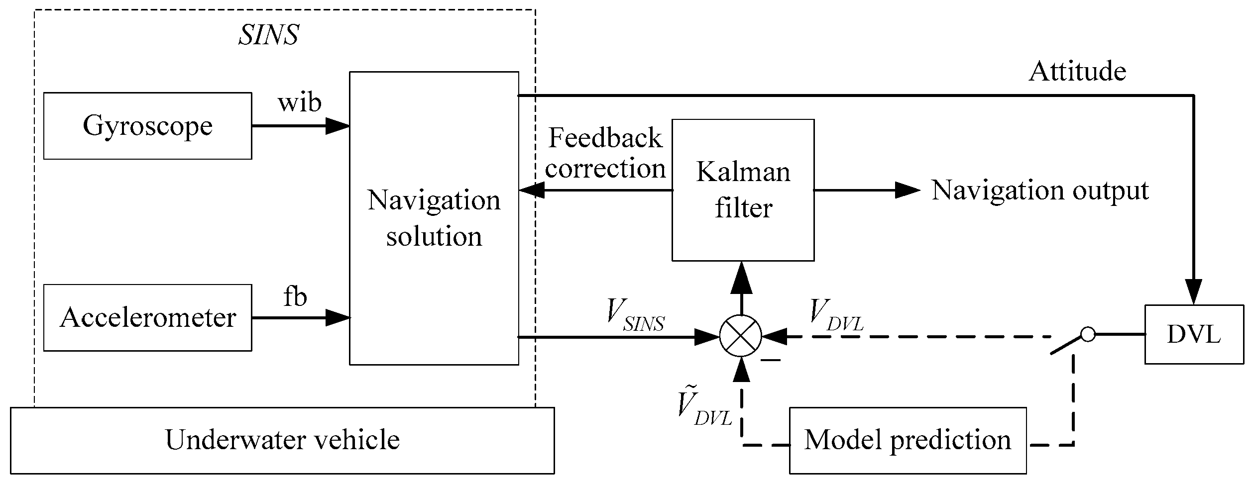
However, traditional LS-SVM from our previous work cannot be applied to DVL model prediction directly because of the following reasons: (1) Due to the limitations of the algorithms themselves, it is difficult to guarantee the generalization ability of the model for the risk of over-fitting. (2) The existing DVL prediction models only take SINS velocities and their change rates as the input training samples, ignoring the consideration of dynamic attitude angle in DVL modeling. Especially for large maneuvering environments, the previous models cannot accurately describe the error characteristics of DVL. Considering the above issues, the FMLS-SVM-based method is proposed in this paper. Figure 1 gives the system structure of DVL model prediction in SINS/DVL.

As shown in Figure 1, the structure of this paper is organized as follows. The SINS dynamic error model and DVL error model of SINS/DVL integrated navigation are established in Section 2. The fuzzy multi-output least squares support machine algorithm is presented in Section 3. The prediction model of DVL based on FMLS-SVM is designed in Section 4. The experiment verification and analysis of the proposed method are realized in Section 5. Finally, the conclusion is drawn in Section 6.

The contributions of this paper can be summarized as follows: (1) Considering that both the input sample and output sample are multi-dimensional, the single-output LS-SVM model is extended to the multi-output LS-SVM model. (2) The fuzzy theory is applied to MLS-SVM to increase its robustness and generalization ability. (3) This method defines the fuzzy membership function benefit from the idea of the K nearest neighbor algorithm, making full use of the constraint relation between the training samples. The proposed membership function can realize self-adaptive control without setting any liminal values in advance. (4) This method creatively adds the dynamic attitude angles to the prediction model to further improve the generalization ability of the prediction model for large maneuvering environments. (5) All experimental data are obtained from the UUV experimental platform. Both simulation analysis and online verification are carried out to validate the effectiveness of the proposed method.

2. SINS/DVL Integrated Navigation Model

2.1. SINS Dynamic Error Model

In order to describe the SINS/DVL integrated navigation model accurately, the nonlinear model with a large misalignment angle is adopted in this paper. We set the right-front-up (RFU) frame as the vehicle frame (denoted as $b$ frame) and the east-north-up (ENU) geographic coordinate as the navigation frame (denoted as $n$ frame).

The acquisition and acquisition accuracy of initial attitude information (pitch, roll, and heading) directly affects the accuracy of dead reckoning. Since the pipeline inertial locator usually uses MEME gyro devices, the measurement accuracy is low and it is difficult to be sensitive to the angular velocity information of the Earth’s rotation, which cannot be used. The natural local gravitational acceleration vector and the angular velocity vector of the Earth’s rotation are used to determine the initial attitude through the method of two-vector attitude determination. The MEMS accelerometer can be sensitive to the local gravitational acceleration, and the initial horizontal attitude information can be obtained by measuring the output value of the accelerometer. After the system starts to work, the inertial locator is stationary for 2 min, and the sampled acceleration data are averaged. The attitude and velocity error equation of SINS [31] can be expressed as:

$$\left\{\begin{array}{c}\delta {\dot{\mathit{v}}}^n=\left[{\mathit{f}}^n\times \right]\mathit{\varphi }-\left(2{\mathit{\omega }}_{ie}^n+{\mathit{\omega }}_{en}^n\right)\times \delta {\mathit{v}}^n+{\mathit{C}}_b^n\mathit{\nabla }\\ \dot{\mathit{\varphi }}=\left({\mathit{\omega }}_{ie}^n+{\mathit{\omega }}_{en}^n\right)\times \mathit{\varphi }+\left(\delta {\mathit{\omega }}_{ie}^n+\delta {\mathit{\omega }}_{en}^n\right)-{\mathit{C}}_b^n\mathit{\epsilon }\end{array}\right.,$$

(1)

where $\delta {\mathit{v}}^n$ is the velocity error. $\mathit{\varphi }$ is the attitude error, and ${\mathit{f}}^n$ is the specific force in the $n$ frame. ${\mathit{C}}_b^n$ is the transformation matrix from the $b$ frame to $n$ frame. ${\mathit{\omega }}_{ie}^n$ is the projected angular velocity of the earth frame (denoted as $e$ frame) relative to the inertial frame (denoted as $i$ frame) in the $n$ frame. ${\mathit{\omega }}_{en}^n$ is the projected angular velocity of the $n$ frame relative to the $e$ frame in the $n$ frame. $\mathit{\epsilon }$ and $\mathit{\nabla }$ are the gyroscope drift and accelerometer bias in the $b$ frame, respectively.

In general, $\mathit{\epsilon }$ and $\mathit{\nabla }$ are modeled as random constants:

$$\left\{\begin{array}{c}\dot{\mathit{\nabla }}=0\\ \dot{\mathit{\epsilon }}=0\end{array}\right..$$

(2)

Seeing that the position error in the SINS/DVL integrated navigation system is unobservable, the error state vector of the Kalman filter is defined as:

$$\mathit{x}=\left[\delta v_E \delta v_N \delta v_U {\varphi }_E {\varphi }_N {\varphi }_U {\nabla }_x {\nabla }_y {\nabla }_z {\epsilon }_x {\epsilon }_y {\epsilon }_z\right],$$

(3)

where $\delta V_E$, $\delta V_N$, and $\delta V_U$ are velocity errors. ${\varphi }_E$, ${\varphi }_N$, and ${\varphi }_U$ are attitude errors.

According to Formulas (1) and (2), the system equation of the Kalman filter can be given as follows

$$\dot{\mathit{x}}=\mathit{F}\mathit{x}+\mathit{w},$$

(4)

where $\mathit{F}$ is the state transition matrix. $\mathit{w}$ is the state noise matrix.

2.2. DVL Error Model

The velocity output by DVL is used as the external velocity reference of the SINS/DVL integrated navigation system, and the measurement equation can be constructed as:

$$\mathit{z}={\tilde{\mathit{v}}}_{INS}^n-{\tilde{\mathit{C}}}_b^n{\mathit{v}}_{DVL}^b,$$

(5)

where ${\tilde{\mathit{v}}}_{INS}^n$ is the velocity output by SINS in the $n$ frame. ${\mathit{v}}_{DVL}^b$ is the projected velocity output by DVL in the $b$ frame. ${\tilde{\mathit{C}}}_b^n$ is the direction cosine matrix in error, and the definition is presented by Formula (6):

$${\tilde{\mathit{C}}}_b^n=\left[{\mathit{I}}_{3\times 3}-\mathit{\varphi }\times \right]{\mathit{C}}_b^n.$$

(6)

To obtain ${\mathit{v}}_{DVL}^b$, the following conversion is required.

$${\mathit{v}}_{DVL}^b={\mathit{C}}_d^b\left(\mathit{K}{\mathit{v}}_{DVL}^d+\delta {\mathit{v}}_d\right),$$

(7)

where ${\mathit{v}}_{DVL}^d$ is the DVL velocity output in the Doppler instrumental frame (denoted as $d$ frame). ${\mathit{C}}_d^b$ is the transformation matrix from the $d$ frame to $b$ frame, that is, ${\mathit{C}}_d^b=\left(\mathit{I}-\mathit{e}\times \right)$, in which $\mathit{e}$ is the installation error vector between the $d$ frame and $b$ frame. $\delta {\mathit{v}}_d$ and $\delta \mathit{K}$ denote the random measurement error vector and the scale factor error vector by DVL, respectively. The scale factor matrix $\mathit{K}$ is given by:

$$\mathit{K}=diag\left(1+\delta K_x,1+\delta K_y,1+\delta K_z\right),$$

(8)

where $diag(\cdot )$ denotes the diagonal matrix.

Substituting Formulas (6) and (7) in Formula (5) yields:

$$\mathit{z}=\delta {\mathit{v}}^n-\left[\left({\mathit{C}}_b^n{\mathit{C}}_d^b\mathit{K}{\mathit{v}}_{DVL}^d\right)\right]\times \mathit{\varphi }=\mathit{H}x+\mathit{\eta },$$

(9)

where $\mathit{\eta }$ is zero-mean Gaussian white noise. $\mathit{H}$ can be described by Formula (10).

$$\mathit{H}=\left[{{\mathit{I}}_{3\times 3}-\left({\mathit{C}}_b^n{\mathit{C}}_d^b\mathit{K}{\mathit{v}}_{DVL}^d\right)\times \mathbf{0}}_{3\times 6}\right].$$

(10)

3. Fuzzy Multi-Output Least Squares Support Vector Machine

3.1. Multi-Output LS-SVM

The predicted velocity of DVL is three-dimensional, so the single-output LS-SVM model [17] is extended to the multi-output LS-SVM model. The principle model is derived as follows:

The training samples are given by:

$$\mathit{S}={\left\{{\mathit{x}}_i,{\mathit{y}}_i\right\}}_{i=1}^N,{\mathit{x}}_i\in {\mathit{R}}^d,{\mathit{y}}_i\in {\mathit{R}}^m,$$

(11)

where ${\mathit{x}}_i$ is the input samples and ${\mathit{y}}_i$ is the target samples. It is supposed that $d$ and $m$ denote the dimensions of the given training samples. $N$ is the size of training samples.

The sample input space is mapped to a high-dimensional feature space by a nonlinear mapping function so that the nonlinear regression problem in the input space is transformed into the linear regression problem in the high-dimensional feature space. Based on the risk minimization principle, the regression problem can be described as a constrained optimization problem:

$$\left\{\begin{array}{l}\min \frac{1}{2}{{\displaystyle \sum _{j=1}^m‖{\omega }_j‖}}^2+\frac{1}{2}C{\displaystyle \sum _{i=1}^N{\displaystyle \sum _{j=1}^m{\xi }_{i,j}^2+C_0{\displaystyle \sum _{i=1}^N{\eta }_i}}}\hfill \\ s.t. y_{i,j}={\omega }_j^T\phi \left({\mathit{x}}_i\right)+b_j+{\xi }_{i,j}^{ }, {\eta }_i={\displaystyle \sum _{j=1}^m\left|{\xi }_{i,j}^{ }\right|}\hfill \end{array}\right.,$$

(12)

where $\mathit{\omega }$ is the weight of training samples. $C$ and $C_0$ are penalty coefficients for single output samples and total samples. $\mathit{\eta }$ is the regression error for total samples. $\mathit{\xi }$ is the slack variable. $\mathit{b}$ is the offset component.

Using Lagrange parameter $\mathit{\alpha }$, the Lagrange function is defined as follows:

$$\begin{array}{l}L\left(\mathit{\omega },\mathit{b},\mathit{\xi },\mathit{\alpha }\right)=\frac{1}{2}{{\displaystyle \sum _{j=1}^m‖{\omega }_j‖}}^2+\frac{1}{2}C{\displaystyle \sum _{i=1}^N{\displaystyle \sum _{j=1}^m{\xi }_{i,j}^2+C_0{\displaystyle \sum _{i=1}^N{\eta }_i}}}+\\ {\displaystyle \sum _{i=1}^N{\displaystyle \sum _{j=1}^m{\alpha }_{i,j}\left(y_{i,j}-{\omega }_j^T\phi \left({\mathit{x}}_i\right)-b_j-{\xi }_{i,j}^{ }\right).}}\end{array}$$

(13)

According to the Karush–Kuhn–Tucker (KKT) condition, we obtain:

$$\left\{\begin{array}{l}\raisebox{1ex}{$\partial L$}\!\left/ \!\raisebox{-1ex}{$\partial {\omega }_j$}\right.={\omega }_j-{\displaystyle \sum _{i=1}^N{\alpha }_{i,j}\phi \left({\mathit{x}}_i\right)=0}\hfill \\ \raisebox{1ex}{$\partial L$}\!\left/ \!\raisebox{-1ex}{$\partial b_j$}\right.=-{\displaystyle \sum _{i=1}^N{\alpha }_{i,j}=0}\hfill \\ \raisebox{1ex}{$\partial L$}\!\left/ \!\raisebox{-1ex}{$\partial {\xi }_{i,j}^{ }$}\right.=C{\xi }_{i,j}^{ }-{\alpha }_{i,j}=0\hfill \\ \raisebox{1ex}{$\partial L$}\!\left/ \!\raisebox{-1ex}{$\partial {\alpha }_{i,j}$}\right.={\mathit{y}}_i-{\omega }_j^T\phi \left({\mathit{x}}_i\right)-b_j-{\xi }_{i,j}^{ }=0\hfill \end{array}\right..$$

(14)

By solving the constrained optimization problem and eliminating ${\omega }_j$ and ${\xi }_{i,j}^{ }$, the following linear equations are obtained.

$$\left[\begin{array}{cc}0& {\mathit{e}}^T\\ \mathit{e}& K({\mathit{x}}_i,{\mathit{x}}_j)+C^{-1}\mathit{I}\end{array}\right]\left[\begin{array}{c}{b}_j\\ {\mathit{\alpha }}_j\end{array}\right]=\left[\begin{array}{c}0\\ {\mathit{y}}_j^{\ast }\end{array}\right],$$

(15)

$${\mathit{y}}_j^{\ast }={\mathit{y}}_j^{ }+\frac{C_0}{C}{\mathit{M}}_j,$$

(16)

where $\mathit{I}$ is the identity matrix, that meets $\mathit{I}\in {\mathit{R}}^{N\times N}$. ${\mathit{y}}_j^{ }={\left[y_1,y_2,\dots ,y_N\right]}^{\mathrm{T}}$,${\mathit{\alpha }}_j^{ }={\left[{\alpha }_{1,j},{\alpha }_{2,j},\dots ,{\alpha }_{N,j}\right]}^{\mathrm{T}}$, and $\mathit{e}={\left[1,1,\dots ,1\right]}^{\mathrm{T}}$. $K({\mathit{x}}_i,{\mathit{x}}_j)$ is the kernel function instead of the inner product calculation of nonlinear mapping. $K({\mathit{x}}_i,{\mathit{x}}_j)$ is defined as a Gaussian kernel function. ${\mathit{M}}_j$ is a N-dimension vector given by:

$${\mathit{M}}_j=\left\{\begin{array}{l}1 {\xi }_{i,j}^{ }\ge 0\hfill \\ -1 {\xi }_{i,j}^{ } < 0\hfill \end{array}\right..$$

(17)

Using Formula (15), ${\mathit{\alpha }}_j^{ }$ and $b_j$ are calculated, and the regression function can be obtained by:

$$f^{(j)}(\mathit{x})={\displaystyle \sum _{i=1}^N{\alpha }_{i,j}}K({\mathit{x}}_i,{\mathit{x}}_j)+b_j,j=1,2,\dots ,m.$$

(18)

Since each component of $\mathit{\alpha }$ in MLS-SVM is proportional to the sample error $\mathit{\xi }$, all sample data points will become support vectors. Accordingly, it is too sensitive to noise and outlier points.

3.2. Fuzzy Multi-Output LS-SVM

To eliminate the over-sensitivity of MLS-SVM to outlier points and the resulting over-fitting problem, the fuzzy membership function [23] is introduced to fuzzify the input samples, and different membership values imply different levels of importance. This method is named the fuzzy multi-output least squares support vector machine. Obviously, the standard MLS-SVM can be considered a special case of FMLS-SVM.

It is given that the fuzzy membership value of each sample is ${\mu }_{i,j}\in {\mathit{R}}^{N\times m}$; then, the cost function described in Formula (12) can be rewritten as:

$$\left\{\begin{array}{l}\min \frac{1}{2}{{\displaystyle \sum _{j=1}^m‖{\omega }_j‖}}^2+\frac{1}{2}C{\displaystyle \sum _{i=1}^N{\displaystyle \sum _{j=1}^m{\mu }_{i,j}^{ }{\xi }_{i,j}^2+C_0{\displaystyle \sum _{i=1}^N{\eta }_i}}}\hfill \\ s.t. y_{i,j}={\omega }_j^T\phi \left({\mathit{x}}_i\right)+b_j+{\xi }_{i,j}^{ }, {\eta }_i={\displaystyle \sum _{j=1}^m\left|{\xi }_{i,j}^{ }\right|}\hfill \end{array}\right..$$

(19)

The Lagrange function is designed as:

$$\begin{array}{l}L\left(\mathit{\omega },\mathit{b},\mathit{\xi },\mathit{\alpha }\right)=\frac{1}{2}{{\displaystyle \sum _{j=1}^m‖{\omega }_j‖}}^2+\frac{1}{2}C{\displaystyle \sum _{i=1}^N{\displaystyle \sum _{j=1}^m{\mu }_{i,j}^{ }{\xi }_{i,j}^2+}}\\ C_0{\displaystyle \sum _{i=1}^N{\eta }_i}+ {\displaystyle \sum _{i=1}^N{\displaystyle \sum _{j=1}^m{\alpha }_{i,j}\left(y_{i,j}-{\omega }_j^T\phi \left({\mathit{x}}_i\right)-b_j-{\xi }_{i,j}^{ }\right)}}.\end{array}$$

(20)

Similarly, the following linear equations can be obtained.

$$\left[\begin{array}{cc}0& {\mathit{e}}^T\\ e& K({\mathit{x}}_i,{\mathit{x}}_j)+C^{-1}\mathit{I}\end{array}\right]\left[\begin{array}{c}{b}_j\\ {\mathit{\alpha }}_j\end{array}\right]=\left[\begin{array}{c}0\\ {\mathit{y}}_j^{\ast }\end{array}\right].$$

(21)

By calculating Formula (21), we obtain the regression function. It is known that the key problem is how to design the fuzzy membership function. There is no unified approach to calculate the fuzzy membership function, but the consistent idea is to assign small membership to outlier points or noise so as to identify the outlier points and noise. For a specific model, the fuzzy membership function needs to be designed according to the relationship between the physical characteristics of samples rather than invoking previous functions directly. The specific definition of the fuzzy membership function in this model will be introduced in detail in Section 4.

4. DVL Model Prediction Method Based on FMLS-SVM

Considering the influence of the sensor state in SINS and the motion of the vehicle on the DVL prediction model, this method realizes the online prediction of the DVL model in order to eliminate the interference of other factors as much as possible. When DVL works well, the DVL prediction model is continuously trained at a fixed time interval. When DVL fails, the invalid DVL measurement value can be predicted by the latest prediction model. Until DVL works well again, the prediction model is updated. The specific working mechanism is shown in Figure 2.

In Figure 2, $t_0$ represents the starting time of model training in the case of DVL working well, and $\Delta t$ represents the update time interval of the DVL prediction model. Model_1 and Model_2 are the DVL prediction models at $t_0+\Delta t$ and $t_0+2\Delta t$ time, respectively. When DVL malfunctions at $t_1$ time, the navigation system predicts the DVL measurement value using Model_2. When the DVL returns to working well at $t_2$ time, the prediction model is trained again at the $\Delta t$ time interval. Based on this rule, Model_3 represents the DVL prediction model at $t_2+\Delta t$ time. When DVL works well, the navigation system stores all navigation information within $\Delta t$ time and the latest training model parameters.

In order to clearly understand the training process of the DVL prediction model, it is necessary to define the input and output of the prediction model. The three-dimensional velocities in $n$ frame provided by SINS are selected as the model input, and the three-dimensional velocities in $d$ frame provided by DVL are selected as the model output in [16]. Furthermore, the three-dimensional velocities’ change rate in the $n$ frame provided by SINS is added to the input of the model in [15]. In view of the following two factors, this paper extends the heading angle provided by SINS and its change rate, pitch angle, and roll angle to the input of the prediction model.

(1)

Ignoring the scale factor error of DVL and the installation error between DVL and SINS, the input and output velocities need to be converted to the same frame by an attitude conversion matrix.

(2)

Considering the influence of the attitude dynamic on DVL measurement accuracy, the heading angle and its change rate, pitch angle, and roll angle of the vehicle are required to be modeled.

Based on the above analysis, the input and output of the training sample set are defined as:

$$\left\{\begin{array}{l}{\mathit{x}}_i=\left\{v_E,v_N,v_U,d{v}_E,d{v}_N,d{v}_U,yaw,dyaw,pitch,roll\right\}\hfill \\ {\mathit{y}}_i=\left\{v_{dx},v_{dy},v_{dz}\right\}\hfill \end{array}\right.,$$

(22)

where $v_E,v_N,v_U$ denote velocities in the $n$ frame output by SINS. $d{v}_E,d{v}_N,d{v}_U$ denote velocity change rates in the $n$ frame output by SINS. $yaw,dyaw,pitch,roll$ denote heading, heading change rate, pitch, and roll output by SINS, respectively. $v_{dx},v_{dy},v_{dz}$ denote velocities output by DVL in the $d$ frame.

Since the input and output samples are represented in different frames, the sample data need to be preprocessed, the conversion formula is presented as follows:

$$\left[\begin{array}{c}{v}_{dx1}\\ v_{dy1}\\ v_{dz1}\end{array}\right]={\mathit{C}}_b^n{\mathit{C}}_d^b\left[\begin{array}{c}{v}_{dx}\\ v_{dy}\\ v_{dz}\end{array}\right].$$

(23)

Considering that the velocity provided by SINS and the velocity provided by DVL are both physical quantities to describe the line motion of the vehicle, a new sample is generated by introducing the idea of the K nearest neighbor algorithm to find the nearest k-1 samples for each sample, namely:

$$\left\{\begin{array}{l}\Delta {\mathit{v}}_i=\left\{\Delta v_1,\Delta v_2,\dots ,\Delta v_k\right\}\hfill \\ \mathit{d}{\mathit{v}}_i=\left\{d{v}_1,d{v}_2,\dots ,d{v}_k\right\}\hfill \end{array}\right.,$$

(24)

where $\Delta {\mathit{v}}_i(j=1,2,\dots ,k)\in {\mathit{R}}^3$ represents the difference sequence between the input and output velocities in k samples. $\mathit{d}{\mathit{v}}_i(j=1,2,\dots ,k)\in {\mathit{R}}^3$ represents the difference sequence between the input and output velocity change rates in k samples.

The definition of fuzzy membership can be constructed as:

$${\mu }_{i,j}=1-(1-\theta ){\left(\frac{1}{2}\left(\frac{\Delta {\tilde{v}}_i(j)-\Delta v_{\min }(j)}{\Delta v_{\max }(j)-\Delta v_{\min }(j)}+\frac{d{\tilde{v}}_i(j)-d{v}_{\min }(j)}{d{v}_{\max }(j)-d{v}_{\min }(j)}\right)\right)}^f,$$

(25)

where $\theta$ is a small enough positive number used to control the lower limit of membership. $f$ represents the variation trend of the membership function. $\Delta {\tilde{v}}_i(j)$ represents the average of the $j-th$ element in $\Delta {\mathit{v}}_i$. $\Delta v_{\min }(j)$ and $\Delta v_{\max }(j)$ represent the minimum value and maximum value of the $j-th$ element in $\Delta {\mathit{v}}_i$, respectively. $d{\tilde{v}}_i(j)$ represents the average of the $j-th$ element in $\mathit{d}{\mathit{v}}_i$. $d{v}_{\min }(j)$ and $d{v}_{\max }(j)$ represent the minimum value and maximum value of the $j-th$ element in $\mathit{d}{\mathit{v}}_i$, respectively.

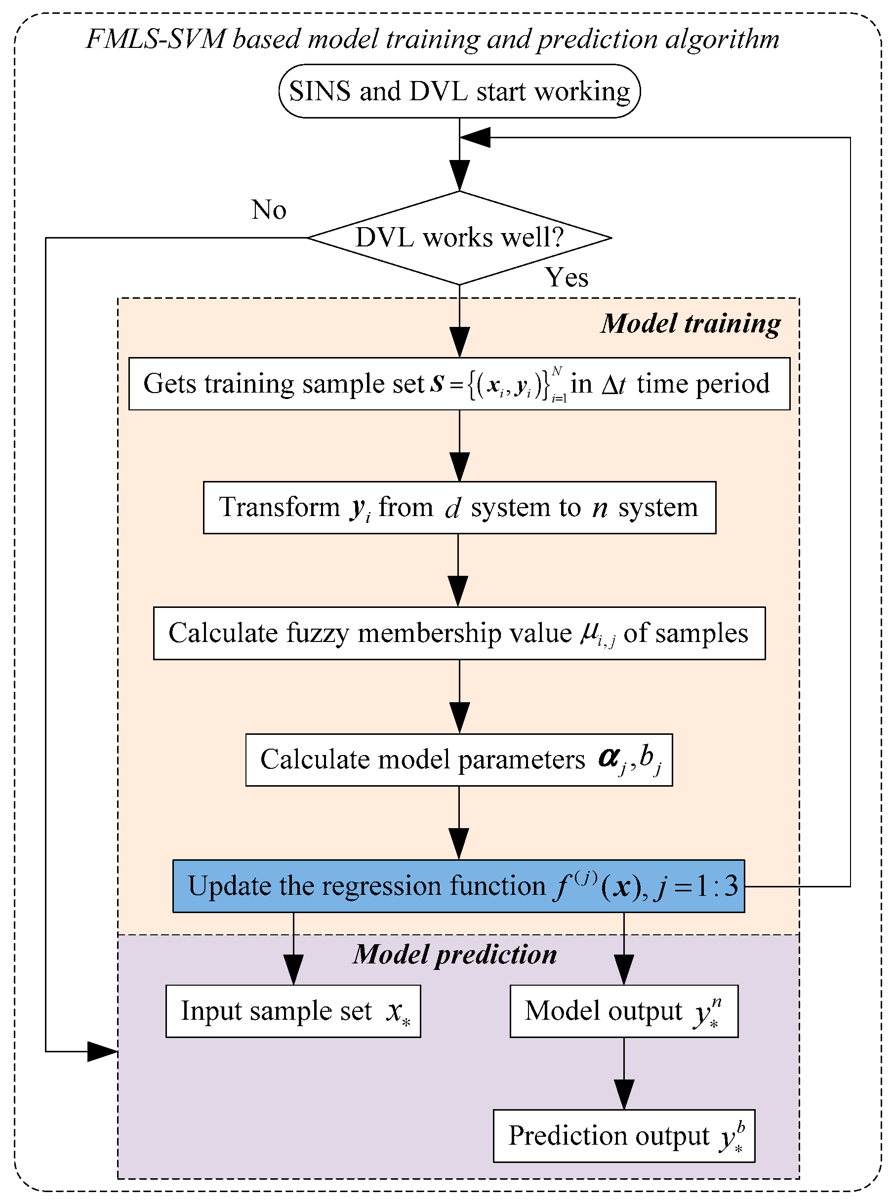
Since the output of the DVL prediction model is expressed in the $n$ frame, it needs to be converted to the $d$ frame by using the attitude transformation matrix. According to the fuzzy multi-output least squares support vector machine model established in Section 3, Figure 3 gives the training and prediction algorithm of the DVL model based on FMLS-SVM.

5. Lake Experiment and Analysis

In order to validate the proposed approach, the lake experiment is undertaken in this study. As shown in Figure 4 and Figure 5, the underwater UUV experiment platform for evaluating the proposed method is equipped with a Doppler velocity log (including a transducer array and an electronic cabinet), high-precision SINS, and GNSS shown in Figure 6. The main specifications of the instruments used in the experiments are listed in

Table 1. Main specifications of the instruments used in the experiment.

Device	Index	Value
Gyroscope	Zero Bias (°/h)	0.01
	$\mathrm{Random} \mathrm{walk} (°/\sqrt{\mathrm{h}})$	0.002
Accelerometer	Zero Bias (mg)	0.1
	$\mathrm{Random} \mathrm{walk} \left(\mathsf{\mu }\mathrm{g}/\sqrt{\mathrm{h}}\right)$	20
DVL	Range (kn)	10
	speed measurement accuracy	5‰
GNSS	positioning accuracy (m)	10
	Speed accuracy (m/s)	0.1

.

In the experiment, the DVL sensor provides three axis velocities of UUV, and FOG-SINS provides the navigation information of UUV. To evaluate the performance of positioning precision, GNSS is employed to provide precise position information as reference values. Two groups of experiments are completed in the experiment, in which UUV is required to be close to the surface of water to ensure the effectiveness of GNSS. Figure 7 gives the trajectory of the experimental vehicle by GNSS.

In order to further validate the performance of the proposed DVL prediction method, both the MLS-SVM-based model and FMLS-SVM-based model are implemented. When DVL works well, the SINS calculating results and the DVL measurements are collected as training samples. Then, the DVL prediction model is updated online with a constantly updated sample set when the DVL works well. If DVL malfunction occurs, the trained prediction model will be applied to predict the DVL measurements. The CPU configuration of the simulation computer is Intel Core i5-1135G7 (2.4 GHz). We simulate via VS2010 software. The small positive number $\theta$ is set to 0.01. In view of the complex signal distribution of the DVL sample, the values of $f$ are set to 2. Considering that the sway period is about 12 s in three scales of sea state and the updating rate of DVL is 1 Hz, the value of $k$ is set to 12. The sample size for the training is 60 s, and the sample set updates online.

Figure 8 and Figure 9 provide the comparison of horizontal velocity measurements under different DVL prediction models in the experiment, and all velocity measurements are presented in the vehicle frame.

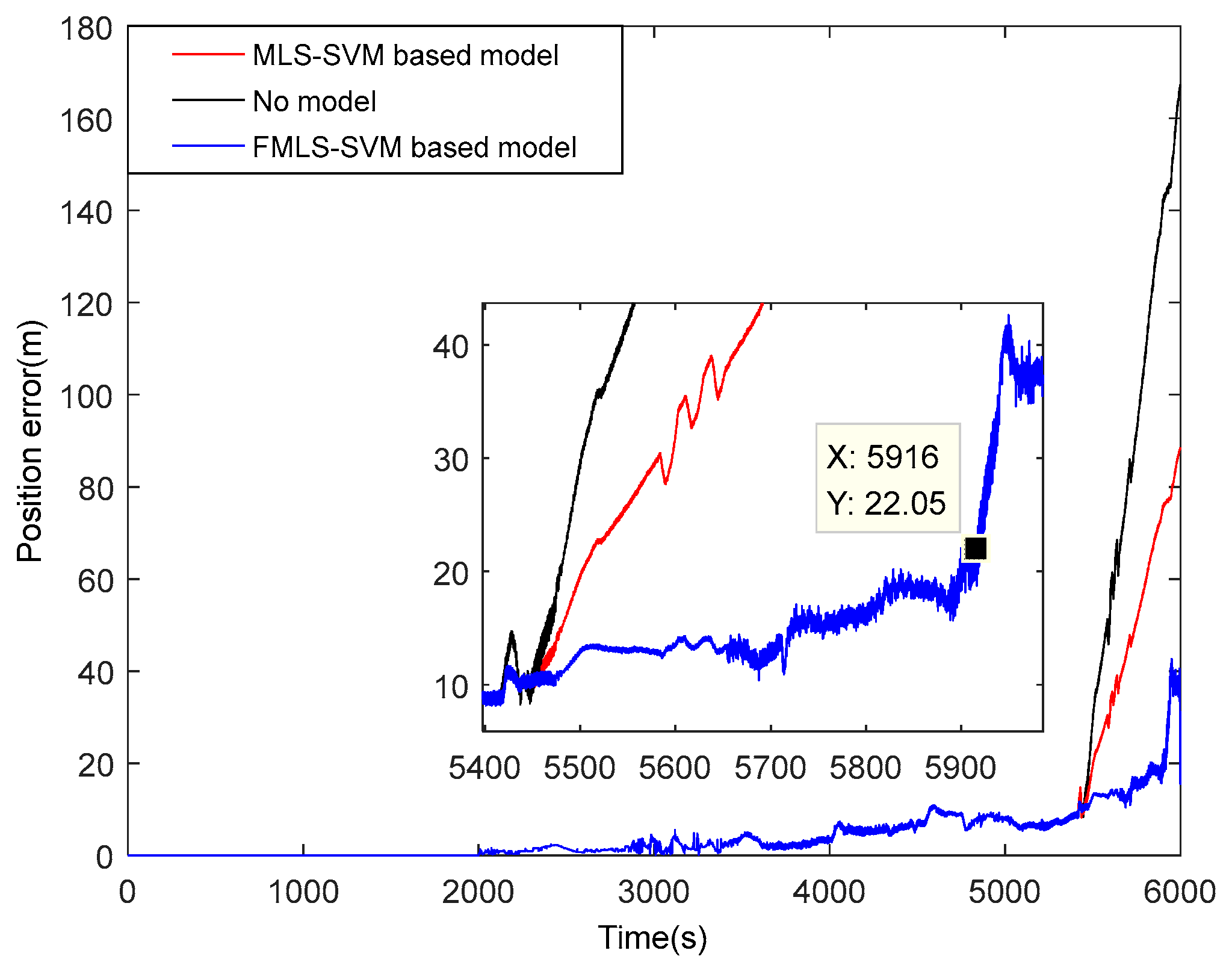
Furthermore, the influence of different DVL prediction models on the positioning accuracy of SINS/DVL is shown in Figure 10.

It can be concluded from Figure 10 that the position errors with the MLS-SVM-based model and FMLS-SVM-based model are decreased by about 60.75% and 83.01%, respectively, compared with no model. The positioning accuracy of the SINS/DVL integrated navigation system is obviously improved by employing the DVL prediction models, in which the position error has been reduced by more than half using the FMLS-SVM-based model compared with the MLS-SVM-based model. Moreover, the CPU running time of DVL prediction models based on the MLS-SVM method and FMLS-SVM method are about 55 μs and 70 μs, respectively. The time of model calculation can meet real-time requirements.

Moreover, it can be seen in Figure 8 and Figure 9 that the time duration of DVL malfunction is from 5416 s to 5654 s, while the time duration of DVL malfunction is considered to be uncertain for complex underwater environments. As we know, the longer the length of DVL malfunction, the poorer the performance of the DVL predictor model. The DVL measurement velocities after 5654 s are forced to be invalid in order to determine the maximum tolerance failure time of the DVL prediction model furtherly. Figure 11 gives the comparison of the positioning accuracy of SINS/DVL under different DVL prediction models.

As described in Figure 11, the navigation accuracy of the SINS/DVL integrated navigation system with the application of the DVL predictor is consistent with that when DVL works well during about the first 500 s (5916 − 5416 s = 500 s). It can be concluded from the experiment results and the above analysis that the proposed DVL predictor can effectively protect SINS/DVL from the effects of short-term malfunction of the DVL.

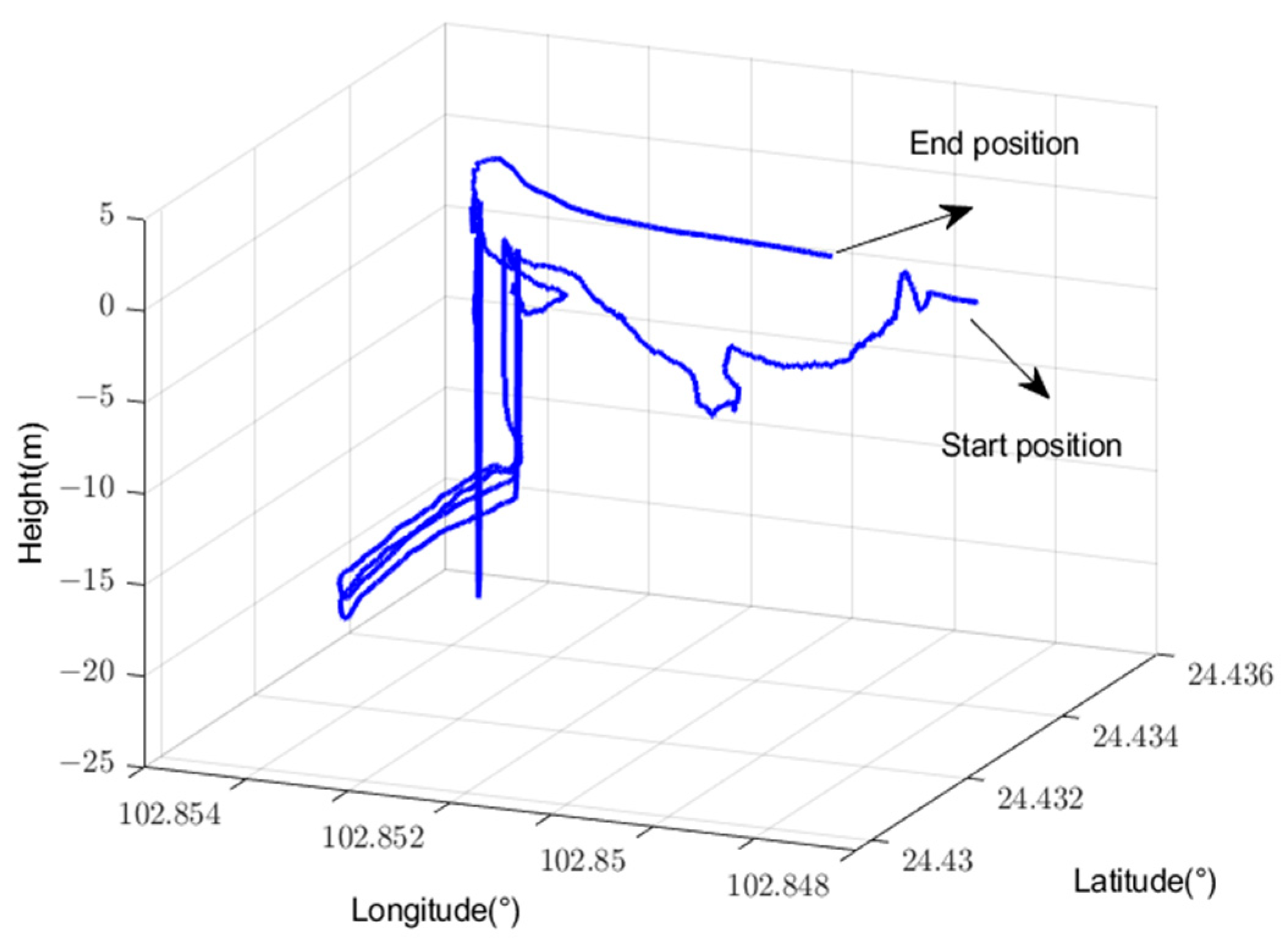
In order to further evaluate the proposed method, another experiment is designed. Different from the previous experiment, we make no restrictions on the route of the UUV experiment platform. In this experiment, a DVL malfunction for 500 s is simulated, and the actual DVL measurement is regarded as the velocity reference to evaluate the accuracy of DVL prediction models. Both the MLS-SVM-based model and FMLS-SVM-based model are applied to the prediction of DVL malfunction. Figure 12 presents the trajectory of UUV indicated by SINS.

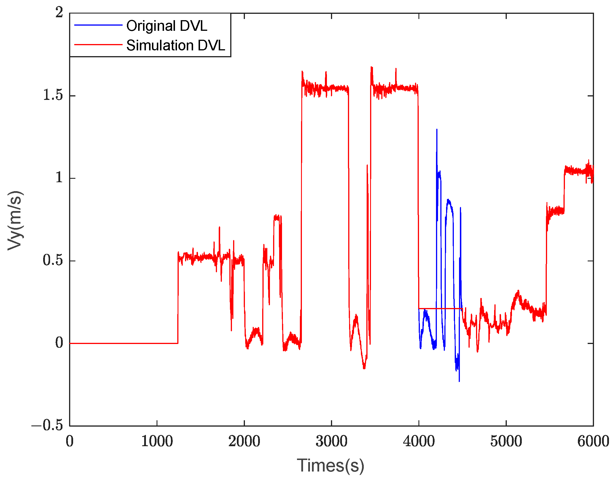
The simulated UUV forward velocity with malfunction by DVL is given in Figure 13, in which the time duration of DVL malfunction is set to 500 s (from 4000 s to 4500 s). Figure 14 gives the comparison of UUV forward velocities under different DVL predictor models.

It can be seen from Figure 14 that the velocity measurements provided by the DVL velocity predictor can effectively restrain the accumulated SINS velocity errors, and the prediction velocity of the FMLS-SVM-based model is closer to the real DVL measurement value than that of the MLS-SVM-based model.

Table 2. The average velocity errors under different prediction models.

Models	Average UUV Forward Velocity Error/m/s
No model	−0.2028
MLS-SVM-based model	0.0627
FMLS-SVM-based model	0.0241

gives the average UUV forward velocity errors under different prediction models from 4000 s to 4500 s.

During the simulation DVL malfunction, the average UUV forward velocity error was reduced by more than half using the FMLS-SVM-based model compared with the MLS-SVM-based model. The results are consistent with the previously reported results.

6. Conclusions

To handle the problem of short-term DVL malfunctions in the SINS/DVL integrated navigation system, this paper proposes an FMLS-SVM-based method to predict invalid DVL measurements. First of all, the single-output LS-SVM model is extended to a multi-output LS-SVM model (MLS-SVM). Since its performance is easily affected by the noises and outlier points, the fuzzy theory is applied to LS-SVM to increase the robustness and generalization ability, and the idea of the K nearest neighbor algorithm is applied to design the fuzzy membership function. For greater adaptability to large maneuvering environments, dynamic attitude angles are added to the prediction model. Furthermore, the online model training and measurement prediction are realized in this method to more accurately describe the DVL prediction model for the present state. When DVL works well, the navigation information from SINS and DVL are employed to train the prediction model. Once the DVL measurement velocity is invalid, the well-trained model is employed to predict the DVL measurements. The lake experiment results and comparison analysis present that the proposed FMLS-SVM predictor has higher estimation accuracy of DVL than the MLS-SVM predictor. For short-term DVL malfunctions, the performance of SINS is impervious, and the tolerance failure time can reach 500 s. Therefore, it can be seen that the proposed DVL prediction model significantly improves the navigation performance of the SINS/DVL integrated navigation system in extreme cases.

In the future, we plan to try more types of intelligent algorithms and their combination forms to apply to this field and conduct field experimental verification.

References

1. Plueddemann, A.J.; Kukulya, A.L.; Stokey, R.; Freitag, L. Autonomous underwater vehicle operations beneath coastal sea ice. IEEE/ASME Trans. Mechatron. 2012, 17, 54–64. [Google Scholar] [CrossRef]
2. Li, W.; Wu, W.; Wang, J.; Wu, M. A novel backtracking navigation scheme for autonomous underwater vehicles. Measurement 2014, 47, 496–504. [Google Scholar] [CrossRef]
3. Pan, X.; Wu, Y. Underwater doppler navigation with self-calibration. J. Navig. 2016, 69, 295–312. [Google Scholar] [CrossRef]
4. Xu, B.; Wang, G.; Bai, J. Optimal design of damping network based on DVL velocity and IMU. Ocean Eng. 2017, 132, 101–113. [Google Scholar] [CrossRef]
5. Paull, L.; Saeedi, S.; Seto, M.; Li, H. AUV navigation and localization: A review. IEEE J. Ocean Eng. 2014, 39, 131–149. [Google Scholar] [CrossRef]
6. Karmozdi, A.; Hashemi, M.; Salarieh, H. Design and practical implementation of kinematic constraints in inertial navigation system-Doppler velocity log (INS-DVL)-based navigation. J. Navig. 2018, 65, 629–642. [Google Scholar] [CrossRef]
7. Hegrenæs, Ø.; Berglund, E. Doppler Water-track Aided Inertial Navigation for Autonomous Underwater Vehicle. In Proceedings of the IEEE OCEANS 2009-EUROPE, Bremen, Germany, 11–14 May 2009; pp. 1–10. [Google Scholar]
8. Martinez, A.; Hernandez, L.; Sahli, H.; Valeriano-Medina, Y.; Orozco-Monteagudo, M.; Garcia-Garcia, D. Model-aided Navigation with Sea Current Estimation for an Autonomous Underwater Vehicle. Int. J. Adv. Robot. Syst. 2015, 12, 103. [Google Scholar] [CrossRef]
9. Hegrenæs, Ø.; Hallingstad, O. Model-Aided INS with Sea Current Estimation for Robust Underwater Navigation. IEEE J. Ocean. Eng. 2011, 36, 316–337. [Google Scholar] [CrossRef]
10. Tal, A.; Klein, I.; Katz, R. Inertial navigation system/Doppler velocity log (INS/DVL) fusion with partial DVL measurements. Sensors 2017, 17, 415. [Google Scholar] [CrossRef]
11. Liu, P.; Wang, B.; Deng, Z.; Fu, M. INS/DVL/PS tightly coupled underwater navigation method with limited DVL measurements. IEEE Sens. J. 2018, 18, 2994–3002. [Google Scholar] [CrossRef]
12. Wang, D.; Xu, X.; Yao, Y.; Zhang, T.; Zhu, Y. A novel SINS/DVL tightly integrated navigation method for complex environment. IEEE Trans. Instrum. Meas. 2020, 69, 5183–5196. [Google Scholar] [CrossRef]
13. Cha, J.; Ju, H.; Park, C.; Yoo, K. Noise covariance adaptation of doppler velocity log considering vehicle’s attitude. In Proceedings of the 18th International Conference on Control, Automation and Systems (ICCAS), PyeongChang, Republic of Korea, 17–20 October 2018; pp. 1303–1306. [Google Scholar]
14. Yao, Y.; Xu, X.; Li, Y.; Zhang, T. A hybrid IMM based INS/DVL integration solution for underwater vehicles. IEEE Trans. Veh. Technol. 2019, 68, 5459–5470. [Google Scholar] [CrossRef]
15. Li, W.; Chen, M.; Zhang, C.; Zhang, L.; Chen, R. A novel neural network-based SINS/DVL integrated navigation approach to deal with DVL malfunction for underwater vehicles. Math. Probl. Eng. 2020, 2020, 2891572. [Google Scholar] [CrossRef]
16. Zhu, Y.; Cheng, X.; Hu, J.; Zhou, L.; Fu, J. A Novel Hybrid Approach to Deal with DVL Malfunctions for Underwater Integrated Navigation Systems. Appl. Sci. 2017, 7, 759. [Google Scholar] [CrossRef]
17. Suykens, J.; Vandewalle, J. Least squares support vector machine classifiers. Neural Process. Lett. 1999, 9, 293–300. [Google Scholar] [CrossRef]
18. Alshammari, S.; Al-Sawalha, M.M.; Shah, R. Approximate Analytical Methods for a Fractional-Order Nonlinear System of Jaulent–Miodek Equation with Energy-Dependent Schrödinger Potential. Fractal Fract. 2023, 7, 140. [Google Scholar] [CrossRef]
19. Shah, N.A.; Hamed, Y.S.; Abualnaja, K.M.; Chung, J.D.; Shah, R.; Khan, A. A Comparative Analysis of Fractional-Order Kaup–Kupershmidt Equation within Different Operators. Symmetry 2022, 14, 986. [Google Scholar] [CrossRef]
20. Wang, J.; Shao, W.; Junseok, K. Combining MF-DFA and LSSVM for retina images classification. Biomed. Signal Process. Control 2020, 60, 101943. [Google Scholar] [CrossRef]
21. Shah, N.A.; Alyousef, H.A.; El-Tantawy, S.A.; Shah, R.; Chung, J.D. Analytical Investigation of Fractional-Order Korteweg–De-Vries-Type Equations under Atangana–Baleanu–Caputo Operator: Modeling Nonlinear Waves in a Plasma and Fluid. Symmetry 2022, 14, 739. [Google Scholar] [CrossRef]
22. Al-Sawalha, M.M.; Ababneh, O.Y.; Shah, R.; Shah, N.A.; Nonlaopon, K. Combination of Laplace transform and residual power series techniques of special fractional-order non-linear partial differential equations. AIMS Math. 2023, 8, 5266–5280. [Google Scholar] [CrossRef]
23. Zadeh, L. Fuzzy sets. Inf. Control 1965, 8, 338–353. [Google Scholar] [CrossRef]
24. Karthick, P.; Mohiuddine, S.; Tamilvanan, K.; Narayanamoorthy, S.; Maheswari, S. Investigations of color image segmentation based on connectivity measure, shape priority and normalized fuzzy graph cut. Appl. Soft Comput. 2023, 139, 110239. [Google Scholar] [CrossRef]
25. Lin, C.; Wang, S. Fuzzy support vector machines. IEEE Trans. Neural Netw. 2002, 13, 464–471. [Google Scholar] [PubMed]
26. Batuwita, R.; Palade, V. FSVM-CIL: Fuzzy support vector machines for class imbalance learning. IEEE Trans. Fuzzy Syst. 2010, 18, 558–571. [Google Scholar] [CrossRef]
27. Rezvani, S.; Wang, X.; Pourpanah, F. Intuitionistic Fuzzy Twin Support Vector Machines. IEEE Trans. Fuzzy Syst. 2019, 27, 2140–2151. [Google Scholar] [CrossRef]
28. Tao, X.; Li, Q.; Ren, C.; Guo, W.; He, Q.; Liu, R.; Zou, J. Affinity and class probability-based fuzzy support vector machine for imbalanced data sets. Neural Netw. 2020, 122, 289–307. [Google Scholar] [CrossRef] [PubMed]
29. Liu, P.; Wang, B.; Deng, Z. A correction method for DVL measurement errors by attitude dynamics. IEEE Sens. J. 2017, 17, 4628–4638. [Google Scholar] [CrossRef]
30. Yao, Y.; Xu, X.; Hou, L.; Deng, K.; Xu, X. A simple and precise correction method for DVL measurements under the dynamic environment. IEEE Trans. Veh. Technol. 2020, 69, 10750–10758. [Google Scholar] [CrossRef]
31. Li, W.; Zhang, L.; Sun, F.; Yang, L.; Chen, M.; Li, Y. Alignment calibration of IMU and Doppler sensors for precision INS/DVL integrated navigation. Optik 2015, 126, 3872–3876. [Google Scholar] [CrossRef]
Figure 1. System structure of DVL model prediction in SINS/DVL.
Electronics 12 02350 g001
Figure 2. Working mechanism of DVL model prediction.
Electronics 12 02350 g002
Figure 3. DVL model training and prediction algorithm based on FMLS-SVM.
Electronics 12 02350 g003
Figure 4. Fiber Optic Gyro Strapdown Inertial Navigation System (FOG-SINS).
Electronics 12 02350 g004
Figure 5. (a) A transducer array. (b) An electronic cabinet.
Electronics 12 02350 g005
Figure 6. The underwater UUV experiment platform.
Electronics 12 02350 g006
Figure 7. The trajectory of UUV indicated by GNSS.
Electronics 12 02350 g007
Figure 8. Comparison of across velocities under different DVL prediction models.
Electronics 12 02350 g008
Figure 9. Comparison of along velocities under different DVL prediction models.
Electronics 12 02350 g009
Figure 10. Comparison of position errors under different DVL prediction models.
Electronics 12 02350 g010
Figure 11. Comparison of position errors under different DVL prediction models with longer tolerance failure time of DVL.
Electronics 12 02350 g011
Figure 12. The trajectory of UUV indicated by SINS.
Electronics 12 02350 g012
Figure 13. The simulated UUV forward velocity with malfunction by DVL.
Electronics 12 02350 g013
Figure 14. Comparison of UUV forward velocities under different prediction DVL models.
Electronics 12 02350 g014