Article

Handling the Complexity of Computing Maximal Consistent Blocks

Department of Artificial Intelligence, University of Information Technology and Management, 35-225 Rzeszów, Poland
Electronics 2023, 12(10), 2295; https://doi.org/10.3390/electronics12102295
Submission received: 10 March 2023 / Revised: 12 May 2023 / Accepted: 17 May 2023 / Published: 19 May 2023
(This article belongs to the Special Issue Knowledge Engineering and Data Mining Volume II)

Abstract

:
The maximal consistent blocks technique, adopted from discrete mathematics, describes the maximal collection of objects, in which all objects are indiscernible in terms of available information. In this paper, we estimate the total possible number of maximal consistent blocks and prove that the number of such blocks may grow exponentially with respect to the number of attributes for incomplete data with “do not care” conditions. Results indicate that the time complexity of some known algorithms for computing maximal consistent blocks has been underestimated so far. Taking into account the complexity, for the practical usage of such blocks, we propose a performance improvement involving the parallelization of the maximal consistent blocks construction method.

1. Introduction

Rough set theory [1,2] is a tool for data mining and knowledge discovery, initially developed for complete information systems [3,4] and then extended for incomplete systems [5,6,7,8,9,10,11,12,13,14,15]. Maximal consistent blocks, as a maximal collection of indiscernible objects, were introduced for incomplete data sets, with missing values represented only as “do not care” conditions, and were used as basic granules to define only ordinary lower and upper approximations in [16]. In [17,18], the definition of maximal consistent blocks was generalized to cover lost values. Furthermore, two new types of approximations were introduced, global probabilistic approximations and saturated probabilistic approximations based on maximal consistent blocks [19,20,21].
Several approaches for computing maximal consistent blocks: the brute force method [22], the recursive method [22] and the hierarchical method [23] were introduced for incomplete data sets with only “do not care” conditions. For incomplete data sets with only lost values, the simplified recursive method based on the property that for such data sets, the characteristic relation is transitive, was provided in [24]. In turn, in [17], the method for computing maximal consistent blocks for arbitrary interpretations of missing attribute values based on a characteristic relation was proposed.
Analysis of the published algorithms for constructing maximal consistent blocks, for data with only “do not care” conditions, revealed two problems. Firstly, the obtained blocks might not be maximal, especially for data sets for which a characteristic relation is not transitive. The second problem is that, in some cases, the reported computational complexity of the algorithms is underestimated [25]. Additionally, in papers [18,26], during the comparison of characteristic sets with generalized maximal consistent blocks in terms of an error rate and complexity of induced rule sets, the authors suggested that characteristic sets can be computed in polynomial time, while computing maximal consistent blocks is associated with exponential time complexity for incomplete data with “do not care” conditions.
In this paper, we estimate the total number of maximal consistent blocks for incomplete data sets. We define a special data set called a k-galaxy set, and we prove that the number of maximal consistent blocks grows exponentially with respect to the number of attributes for incomplete data with all missing attribute values interpreted as “do not care” conditions. Additionally, for the practical usage of this technique of incomplete data set mining, we propose a performance improvement in the form of the parallelization of the maximal consistent blocks construction method.
The paper is organized as follows. In Section 2, Section 3 and Section 4, an appropriate introduction to the used approach for incomplete data mining is presented. In Section 5, the complexity of computing maximal consistent blocks is estimated. Finally, a parallel solution for determining maximal consistent blocks is proposed in Section 6.

2. Incomplete Data

We consider incomplete data sets with two interpretations of missing attribute values—lost values and “do not care” conditions. Lost values, denoted by question marks, are interpreted as values that are erased or not inserted. The “do not care” conditions, denoted by stars, have another interpretation. Here, we assume that the original values are irrelevant so that such values may be replaced by any existing attribute value [27]. The practice of data mining shows that “do not care” conditions are often the results of the refusal to provide a value. For example, some respondents refuse to provide a value of the salary attribute, or, when asked for eye color during the collection of data about a disease, may consider such an attribute as irrelevant and again refuse to specify the value. It is worth noting that there are also other interpretations of missing attribute values, such as not applicable. An example of such a situation can be the value of the salary attribute when a respondent is unemployed. It is important to understand the reasons and distinguish between various types of missing data, such as missing completely at random, missing at random, and missing not at random. Examples can be found in the statistical literature on missing attribute values [28,29].
The incomplete data set, in the form of a decision table, is presented in Table 1. The rows of the decision table represent cases or objects. The set of all cases is called the universe and is denoted by U. Table 1 shows U = {1, 2, 3, 4, 5, 6, 7, 8}. The independent variables are called attributes and are denoted by A. In Table 1, Mileage, Accident and Equipment are the attributes. The set of all values of the attribute a is called a domain of a and is denoted by V a . In Table 1, V E q u i p m e n t = { l o w , h i g h } . The dependent variable Buy is called a decision. The set of all cases with the same decision value is called a concept. In Table 1, there are two concepts, the set {1, 2, 3, 4} of all cases, where the value of Buy is yes and the other set {5, 6, 7, 8}, where the value of Buy is no.
The value v of the attribute a for the case x is denoted by a ( x ) = v . A block of the attribute–value pair, denoted by [ ( a , v ) ] , is the set of all cases from U that for the attribute a have the value v, { x U | a ( x ) = v } .
We consider two interpretations of missing attribute values: lost values denoted by ? and “do not care” conditions denoted by ∗ in Table 1. The set of all cases from U that for the attribute a have lost values { x U | a ( x ) = ? } is denoted by [ ( a , ? ) ] , whereas the set of all cases from U that for the attribute a have “do not care” conditions { x U | a ( x ) = } is denoted by [ ( a , ) ] .
For incomplete decision tables, the definition of a block of an attribute–value pair is modified as follows [27]:
If for an attribute a and a case x, a ( x ) = ? , then the case x should not be included in any blocks [ ( a , v ) ] for all values v of the attribute a;
If for an attribute a and a case x, a ( x ) = , then the case x should be included in blocks [ ( a , v ) ] for all specified values v of the attribute a.
For Table 1, all the blocks of attribute–value pairs are as follows:
  • [ ( M i l e a g e , m e d i u m ) ] = { 1 , 4 , 6 , 8 } ,
  • [ ( M i l e a g e , l o n g ) ] = { 3 , 5 , 6 } ,
  • [ ( A c c i d e n t , y e s ) ] = { 1 , 4 , 5 , 6 , 7 , 8 } ,
  • [ ( A c c i d e n t , n o ) ] = { 2 , 3 , 4 , 6 , 7 , 8 } ,
  • [ ( E q u i p m e n t , l o w ) ] = { 1 , 2 , 4 , 7 } ,
  • [ ( E q u i p m e n t , h i g h ) ] = { 2 , 6 , 8 } .

3. Characteristic Relation

In an incomplete decision table, for B A , the objects of the pair ( x , y ) U are considered similar in terms of the B-characteristic relation R ( B ) defined as follows [12]:
( x , y ) R ( B ) i f a n d o n l y i f y K B ( x ) ,
where K B ( x ) is the characteristic set, i.e., the smallest set of cases that are indistinguishable from x U , for all attributes from B A . For incomplete decision tables, the characteristic set is defined as follows [11]:
If a ( x ) is specified, then K ( x , a ) is the block [ ( a , a ( x ) ) ] of the attribute a and its value a ( x ) ;
If a ( x ) = ? or a ( x ) = , then K ( x , a ) = U .
For the data set from Table 1 and B = A , the characteristic sets are as follows:
  • K A ( 1 ) = { 1 , 4 } ,
  • K A ( 2 ) = { 2 , 3 , 4 , 6 , 7 , 8 } ,
  • K A ( 3 ) = { 3 , 6 } ,
  • K A ( 4 ) = { 1 , 4 } ,
  • K A ( 5 ) = { 5 , 6 } ,
  • K A ( 6 ) = { 2 , 6 , 8 } ,
  • K A ( 7 ) = { 1 , 2 , 4 , 7 } ,
  • K A ( 8 ) = { 6 , 8 } .
The characteristic relation is R ( A ) = {(1, 1), (1, 4), (2, 2), (2, 3), (2, 4), (2, 6), (2, 7), (2, 8), (3, 3), (3, 6), (4, 1), (4, 4), (5, 5), (5, 6), (6, 2), (6, 6), (6, 8), (7, 1), (7, 2), (7, 4), (7, 7), (8, 6), (8, 8)}.

4. Maximal Consistent Blocks

Maximal consistent blocks were introduced for incomplete data sets, in which all missing attribute values are “do not care” conditions, in [16]. The set X, X U , is consistent with respect to B, B A , if ( x , y ) R ( B ) for any x , y X . Maximal consistent blocks were defined as a maximal collection of objects, in which all objects are consistent. If there does not exist a subset Y U such that X Y , and Y is consistent with respect to B, then X is called a maximal consistent block of B. The set of all maximal consistent blocks of B is denoted by C ( B ) . Following [16], the set of all maximal B-consistent blocks, which include an object x U , is denoted by C ( B ) ( x ) .
The definition of maximal consistent blocks, extended to two interpretations of missing attribute values, lost and “do not care” conditions, was introduced in [18]. The set X, X U is consistent with respect to B, B A , if ( x , y ) R ( B ) for any x , y X . If there does not exist a consistent subset Y of U such that X is a proper subset of Y, the set X is called a maximal consistent block of B.
For the data set from Table 1 and B = A , the set C ( A ) of all maximal consistent blocks of A is { { 1 , 4 } , { 2 , 6 } , { 2 , 7 } , { 3 } , { 5 } , { 6 , 8 } } . The collections of maximal consistent blocks with respect to objects determined by A are as follows:
  • C ( A ) ( 1 ) = { { 1 , 4 } } ,
  • C ( A ) ( 2 ) = { { 2 , 6 } , { 2 , 7 } } ,
  • C ( A ) ( 3 ) = { { 3 } } ,
  • C ( A ) ( 4 ) = { { 1 , 4 } } ,
  • C ( A ) ( 5 ) = { { 5 } } ,
  • C ( A ) ( 6 ) = { { 2 , 6 } , { 6 , 8 } } ,
  • C ( A ) ( 7 ) = { { 2 , 7 } } ,
  • C ( A ) ( 8 ) = { { 6 , 8 } } .
The relation S ( B ) , B A and x , y U , formed from all possible pairs ( x , y ) such that x and y are members of the same maximal B-consistent block, is called implied by the family C ( B ) of maximal consistent blocks. The relation S ( B ) is symmetric. For data sets with all missing attribute values interpreted as lost, the relation S ( B ) is transitive [18]. For the data set from Table 1, S ( A ) = {(1, 1), (1, 4), (2, 2), (2, 6), (2, 7), (3, 3), (4, 1), (4, 4), (5, 5), (6, 2), (6, 6), (6, 8), (7, 2), (7, 7), (8, 6), (8, 8)}.

5. Estimation of the Number of Maximal Consistent Blocks

For a data set with all missing attribute values interpreted as lost, a family C ( B ) of all maximal consistent blocks is a partition on U [18].
Properties of maximal consistent blocks for data sets with missing attribute values interpreted as “do not care” conditions were explored in [16] and other papers [22,23]. However, the estimation of the number of possible maximal consistent blocks is an open problem. In this paper, we show that such a number may exponentially grow with respect to the number of attributes.
Proposition 1.
For a data set in which all attribute values are missing and interpreted as “do not care” conditions, the total number of maximal consistent blocks is equal to 1.
Proof. 
This follows directly from the definition of maximal consistent blocks. □
Proposition 2.
For a data set with | U | = 1, the total number of maximal consistent blocks is equal to 1.
Proof. 
This follows directly from the definition of maximal consistent blocks. □
In order to estimate the number of possible maximal consistent blocks for incomplete data sets with all missing attribute values interpreted as “do not care” conditions, we introduce a special data set, which we call a k-galaxy set. Let | A | = k , V a = { 1 , 2 , , k } for all a A . The set is a k-galaxy set if a j ( i ) = j when k · ( j 1 ) < i k · j ; otherwise, a j ( i ) = for any i { 1 , 2 , , k 2 } and j { 1 , , k } . ’·’ denotes a standard arithmetic multiplication operation.
An example of a k-galaxy set (k = 3) is shown in Table 2.
For the k-galaxy set (k = 3) from Table 2, the set of all maximal consistent blocks of A is {{1, 4, 7}, {1, 4, 8}, {1, 4, 9}, {1, 5, 7}, {1, 5, 8}, {1, 5, 9}, {1, 6, 7}, {1, 6, 8}, {1, 6, 9}, {2, 4, 7}, {2, 4, 8}, {2, 4, 9}, {2, 5, 7}, {2, 5, 8}, {2, 5, 9}, {2, 6, 7}, {2, 6, 8}, {2, 6, 9}, {3, 4, 7}, {3, 4, 8}, {3, 4, 9}, {3, 5, 7}, {3, 5, 8}, {3, 5, 9}, {3, 6, 7}, {3, 6, 8}, {3, 6, 9}}.
For a set X, | X | denotes the cardinality of X.
Lemma 1.
For a k-galaxy set, | C ( { a } ) | is equal to k, where a A .
Proof. 
If a A and V a = { 1 , 2 , , k } then a ( x ) a ( y ) for any x , y U , x y . This means that { x } is consistent with respect to a. Therefore, from the definition of maximal consistent blocks, there are k maximal consistent blocks with respect to a. □
For instance, in Table 2, the set of maximal consistent blocks with respect to Attribute 1 from the example of a k-galaxy set for k = 3 is {{1, 4, 5, 6, 7, 8, 9}, {2, 4, 5, 6, 7, 8, 9}, {3, 4, 5, 6, 7, 8, 9}}.
Lemma 2.
For a k-galaxy set, let j , v { 1 , , k } . The set C ( { a j } ) ( v ) is equal to { x | a j ( x ) = v } x = 1 k · ( j 1 ) { x } x = k · j + 1 k 2 { x } , where a j A .
Proof. 
Let a A , v { 1 , , k } and X ( v ) = { x | a ( x ) = v a ( x ) = } . For any x , y X ( v ) , x y , x and y are consistent with respect to a; if a ( x ) = v , then a ( y ) = , so X ( v ) is a consistent block. Moreover, there does not exist z U \ X ( v ) such that a ( z ) = v . This means that objects with values belonging to V a are inconsistent. Therefore, X ( v ) is a maximal consistent block with respect to the attribute a.
Any attribute of a k-galaxy set contains k inconsistent objects belonging to V a and remaining k 2 k objects of the type [ ( a , ) ] . Hence, each C ( { a } ) ( v ) includes exactly one object with a specified value v and k 2 k objects [ ( a , ) ] , and thus | C ( { a } ) ( v ) | is equal to 1 + k 2 k . □
In Lemma 3 and Proposition 3, provided below, we use Property 5 from [16] which states that the set of maximal consistent blocks can be updated sequentially depending on the currently analyzed set of attributes. Let a , b B A , x U , v a , v b { 1 , , k } , X a { x | a ( x ) = v a } and X b { x | b ( x ) = v b } , and from the definition of a k-galaxy set, X a X b = .
Lemma 3.
For a k-galaxy set, the cardinality of each maximal consistent block of C ( B ) is the same, equaling 1 + k 2 k ( k 1 ) · ( | B | 1 ) , B A .
Proof. 
For any x , y U , x y , { x , y } is consistent with respect to { a , b } if x X a and y X a or y X b and x X b . From Lemma 2, the C ( { a } ) includes exactly one object with a specified value v a and k 2 k objects [(a, *)]. Thus, for { a , b } , the set of k 2 k objects [(a, *)] is reduced by k objects belonging to X b . Additionally, based on the construction of a k-galaxy set, the objects in X a as well as in X b are discernible, so the number of elements in C ( { a , b } ) is k 1 less than in C ( { a } ) . Hence, increasing the number of attributes by one reduces the number of elements of C ( B ) by k 1 . In consequence, if B = A , the number of elements of all C ( B ) is reduced to k. □
For instance, in Table 2, k = 3, X A t t r i b u t e 1 = { 1 , 2 , 3 } , X A t t r i b u t e 2 = { 4 , 5 , 6 } the sets {1, 4}, {1, 5}, {1, 6}, {2, 4}, {2, 5}, {2, 6}, {3, 4}, {3, 5} and {3, 6} are consistent with respect to {Attribute1, Attribute2}, and all mentioned sets belong to R(Attribute1, Attribute2) (see Section 4). For the set C ( { A t t r i b u t e 1 } ) is {{1, 4, 5, 6, 7, 8, 9}, {2, 4, 5, 6, 7, 8, 9}, {3, 4, 5, 6, 7, 8, 9}}, each block contains one object with a specified value belonging to V A t t r i b u t e 1 and six objects of the type [(Attribute 1, *)], so | C ( { a } ) | = 7 (see Table 3). The set C ( { A t t r i b u t e 1 , A t t r i b u t e 2 } ) is {{1, 4, 7, 8, 9} {1, 5, 7, 8, 9}, {1, 6, 7, 8, 9}, {2, 4, 7, 8, 9}, {2, 5, 7, 8, 9} {2, 6, 7, 8, 9}, {3, 4, 7, 8, 9}, {3, 5, 7, 8, 9}, {3, 6, 7, 8, 9}}, and each block contains two objects with a specified value—the first belonging to V A t t r i b u t e 1 and the second belonging to V A t t r i b u t e 2 —and three objects [(Attribute 1, *),(Attribute 2, *)]. Therefore, | C ( { a , b } ) | = 5 (see Table 4). The number of elements in C ( { a , b } ) is reduced by ( k 1 ) objects with respect to V A t t r i b u t e 2 . Finally, each block of the C ( A ) , presented above, contains three elements and is reduced again by k 1 objects with respect to V A t t r i b u t e 3 .
Proposition 3.
For a k-galaxy set | C ( A ) | = k k .
Proof. 
For any a A from Lemma 1, | C ( { a } ) | = k . For any x , y U , x y , { x , y } is consistent with respect to { a , b } if x X a and y X a or x X b and y X b . Additionally, based on the construction of a k-galaxy set, the objects in X a as well as in X b are discernible, so each of the k objects belonging to X a is consistent with each of the k objects belonging to X b . Hence, there are k · k consistent blocks with respect to the attributes {a, b}. Objects such that { x | a ( x ) = a n d b ( x ) = } are added to every consistent block with respect to the set of attributes { a , b } . From Lemma 3, all of the blocks have the same number of elements. There are no subsets that are consistent with respect to the set of attributes { a , b } . The obtained blocks are maximal consistent blocks. Extending the set of analyzed attributes by another attribute increases the number of maximal consistent blocks k times, and thus, the number of maximal consistent blocks for the entire k-galaxy set is k k . □
Therefore, in the worst case, the time complexity of computing maximal consistent blocks is O ( n n ) , where n is the number of objects in a data set. This result indicates that the time complexity of some known algorithms for computing maximal consistent blocks was underestimated so far, and their authors suggest that the mentioned problem is associated with polynomial time complexity [22,23].

6. Parallelization of the Maximal Consistent Blocks Computations

The idea of the sequential update of the set of maximal consistent blocks based on Property 5 from [16] proposed in [25] is more effective than the commonly used method of constructing the blocks. However, the subsets merging, which removes subsets by performing comparisons between two sets (the current set of maximal consistent blocks obtained so far and the new one built for the next attribute), has a significant impact on the overall performance. Thus, the usage of maximal consistent blocks in mining real data with a large number of missing values or/and many attributes requires additional improvements. Here, a solution based on parallel processing is proposed.
Due to the fact that the subset is a transitive relation, the merge procedure can apply subset elimination in any order; in particular, merged sets of consistent blocks can be processed in pairs at the same time.
Let A = { a 1 , , a n } and | C ( { a 1 } ) | is equal to k 1 . Thus, the BuildProcedure splits the set of all cases U into a set of k 1 maximal consistent blocks with respect to the first attribute (see Figure 1). Then the k 1 blocks are divided in pairs into a batch of ( k 1 2 + k 1 mod 2 ) separate tasks that are executed simultaneously. In the first batch, the BuildProcedure is called for each block of the pair and the next attribute a 2 , then the resulting sets are merged. The C 1 , C k 1 sets of blocks, being the results of the entire batch, are divided in pairs into ( k 1 4 + k 1 mod 2 ) separate merging tasks and the next batch is formed. The merging continues until a single set of k 2 maximal consistent blocks is obtained. Then the set is divided in pairs into a batch of ( k 2 2 + k 2 mod 2 ) tasks and the computations are performed for the attribute a 3 . The processing is repeated until all the attributes in the data set are taken into account.
In the evaluation of the parallel computation, two aspects should be considered: speedup—the improvement in running time due to parallelism; and efficiency—the ratio of work done by a parallel algorithm to work done by a sequential algorithm [30]. As indicated above, in the worst case in the sequential algorithm, the time complexity of computing maximal consistent blocks is O ( n n ) , where n is the number of objects in a data set. The proposed approach is a synchronized parallel algorithm [31]. The tasks are parallelized in batches. The results of each task from the given batch are not independent and have to be merged. This merging continues in subsequent batches of parallelized tasks until a single set of maximal consistent blocks is obtained. The processes are synchronized at the end of each batch. In the most optimistic scenario, in which all tasks in a batch are executed at the same time, the total number of batches (which can be estimated as k / 2 for each attribute) determines the efficiency. In practice, however, the efficiency is reduced by the fact that p 1 processes have to wait for the processes executing the slowest task in a batch. Therefore, in the worst case, the relative improvement compared to the sequential algorithm is O ( n n 2 ) .
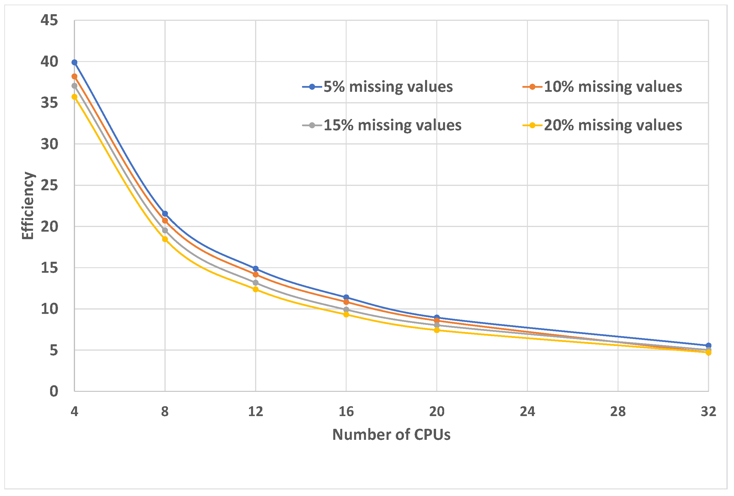
For the demonstration of the real values of the efficiency, the abalone data set with all missing attribute values interpreted as “do not care” conditions was selected, due to the fact that during the experiments performed, using the sequential algorithm, this set turned out to be the most demanding one [25]. The analysis was conducted using 4, 6, 8, 12, 16, 20 and 32 processors. The abalone data set contained 4177 observations and 8 attributes. The “do not care” conditions data sets were prepared by randomly replacing 5%, 10%, 15%, 20% of existing specified attribute values with the “*”s. Results of the analysis are presented in Figure 2 and Figure 3. The speedup does not increase linearly with the number of processors; instead, it tends to saturate. The efficiency drops as the number of processors increases. For parallel systems, this observation is called Amdahl’s law [32]. However, the results show a general increase in the speed (performance) of the parallel approach compared to the sequential computing of maximal consistent blocks. The proposed parallel algorithm includes operations that need to be executed sequentially and the increase in processing speed obtained due to the parallelization of the algorithm is limited by these sequential operations.

7. Conclusions

The idea of a maximal consistent block is adopted from discrete mathematics and describes the maximal collection of objects, in which all objects are similar [16]. In this paper, we prove that the total number of maximal consistent blocks for incomplete data with all missing attribute values interpreted as “do not care” conditions, in the worst case, depends exponentially on the number of attributes. More specifically, the time complexity of computing these blocks may be estimated as O ( n n ) . The results of our work indicate that the time complexity of some known algorithms for computing maximal consistent blocks has been underestimated so far. Furthermore, taking into account the complexity of maximal consistent block calculations, adapting the implementation for parallel computing is proposed. Our experiments show an overall increase in speed (performance) of the parallel approach compared to sequential computations of maximal consistent blocks. However, due to the definition of the blocks, full parallelism does not seem possible. The proposed parallel algorithm consists of operations that must be performed sequentially—synchronized batches of parallel tasks. However, none of the algorithms for calculating maximal consistent blocks available in the literature is ready to be used in parallel computing. The presented solution is the first approach.
It is also worth mentioning that the problem of the complexity of computing maximal consistent blocks has not yet been studied in the available literature. The estimation of the worst-case of such calculations makes it possible to determine their impact on a system’s performance and indicates the upper limit of resources required in practical applications. In the future, we would like to apply this approach in the module of incomplete data mining of a fall detection system [33]. In systems based on sensors, various types of disturbances may occur, caused, for example, by power failure or battery depletion. Due to the fact that the FRSystem, created in cooperation with the Elderly Care Home in Rzeszow, is dedicated to elderly monitoring, such an extension is required.

Funding

This research received no external funding.

Data Availability Statement

Publicly available datasets were analyzed in this study. This data can be found here: https://archive.ics.uci.edu/ml/index.php.

Conflicts of Interest

The author declares no conflict of interest.

References

  1. Pawlak, Z. Rough sets. Int. J. Comput. Inf. Sci. 1982, 11, 341–356. [Google Scholar] [CrossRef]
  2. Pawlak, Z. Rough Sets. Theoretical Aspects of Reasoning about Data; Kluwer Academic Publishers: Dordrecht, The Netherlands; Boston, MA, USA; London, UK, 1991. [Google Scholar]
  3. Pawlak, Z.; Grzymala-Busse, J.W.; Slowinski, R.; Ziarko, W. Rough sets. Commun. ACM 1995, 38, 89–95. [Google Scholar] [CrossRef]
  4. Pawlak, Z.; Skowron, A. Rough sets: Some extensions. Inf. Sci. 2007, 177, 28–40. [Google Scholar] [CrossRef]
  5. Stefanowski, J.; Tsoukias, A. Incomplete information tables and rough classification. Comput. Intell. 2001, 17, 545–566. [Google Scholar] [CrossRef]
  6. Grzymala-Busse, J.W. Data with missing attribute values: Generalization of indiscernibility relation and rule induction. Trans. Rough Sets 2004, 1, 78–95. [Google Scholar]
  7. Leung, Y.; Wu, W.; Zhang, W. Knowledge acquisition in incomplete information systems: A rough set approach. Eur. J. Oper. Res. 2006, 168, 164–180. [Google Scholar] [CrossRef]
  8. Grzymala-Busse, J.W.; Rzasa, W. Local and global approximations for incomplete data. In Proceedings of the Fifth International Conference on Rough Sets and Current Trends in Computing, Kobe, Japan, 6–8 November 2006; pp. 244–253. [Google Scholar]
  9. Nabwey, H.A. A probabilistic rough set approach to rule discovery. Int. J. Adv. Sci. Technol. 2011, 30, 25–34. [Google Scholar]
  10. Clark, P.G.; Grzymala-Busse, J.W. Experiments on probabilistic approximations. In Proceedings of the 2011 IEEE International Conference on Granular Computing, Kaohsiung, Taiwan, 8–10 November 2011; pp. 144–149. [Google Scholar]
  11. Grzymala-Busse, J.W. Characteristic relations for incomplete data: A generalization of the indiscernibility relation. In Proceedings of the Fourth International Conference on Rough Sets and Current Trends in Computing, Uppsala, Sweden, 1–5 June 2004; pp. 244–253. [Google Scholar]
  12. Grzymala-Busse, J. Three Approaches to Missing Attribute Values: A Rough Set Perspective. In Data Mining: Foundations and Practice; Lin, T.Y., Xie, Y., Wasilewska, A., Liau, C.-J., Eds.; Springer: Berlin/Heidelberg, Germany, 2008. [Google Scholar]
  13. Yao, Y.Y. Probabilistic rough set approximations. Int. J. Approx. Reason. 2008, 49, 255–271. [Google Scholar] [CrossRef]
  14. Qi, Y.S.; Sun, H.; Yang, X.B.; Song, Y.; Sun, Q. Approach to approximate distribution reduct in incomplete ordered decision system. J. Inf. Comput. Sci. 2008, 3, 189–198. [Google Scholar]
  15. Chen, M.; Xia, X. An extended rough set model based on a new characteristic relation. In Proceedings of the IEEE Conference on Granular Computing, Kaohsiung, Taiwan, 8–10 November 2011; pp. 100–105. [Google Scholar]
  16. Leung, Y.; Li, D. Maximal consistent block technique for rule acquisition in incomplete information systems. Inf. Sci. 2003, 153, 85–106. [Google Scholar] [CrossRef]
  17. Clark, P.G.; Gao, C.; Grzymala-Busse, J.W.; Mroczek, T.; Niemiec, R. Characteristic Sets and Generalized Maximal Consistent Blocks in Mining Incomplete Data. In Proceedings of the Rough Sets, IJCRS 2017, Olsztyn, Poland, 3–7 July 2017; Lecture Notes in Computer Science. Volume 10313, pp. 477–486. [Google Scholar]
  18. Clark, P.G.; Gao, C.; Grzymala-Busse, J.W.; Mroczek, T. Characteristic sets and generalized maximal consistent blocks in mining incomplete data. Inf. Sci. 2018, 453, 66–79. [Google Scholar] [CrossRef]
  19. Clark, P.G.; Grzymala-Busse, J.W.; Hippe, Z.S.; Mroczek, T.; Niemiec, R. Global and Saturated Probabilistic Approximations Based on Generalized Maximal Consistent Blocks. In Proceedings of the 15th International Conference on Hybrid Artificial Intelligence Systems (HAIS 2020), Gijón, Spain, 11–13 November 2020; pp. 387–396. [Google Scholar]
  20. Clark, P.G.; Grzymala-Busse, J.W.; Hippe, Z.S.; Mroczek, T.; Niemiec, R. Complexity of rule sets mined from incomplete data using probabilistic approximations based on generalized maximal consistent blocks. In Proceedings of the 24th KES KES Conference, Virtual Event, 16–18 September 2020; pp. 1803–1812. [Google Scholar]
  21. Clark, P.G.; Grzymala-Busse, J.W.; Hippe, Z.S.; Mroczek, T. Mining Incomplete Data Using Global and Saturated Probabilistic Approximations Based on Characteristic Sets and Maximal Consistent Blocks. In Proceedings of the International Joint Conference on Rough Sets (IJCRS 2021), Bratislava, Slovakia, 19–24 September 2021; pp. 3–17. [Google Scholar]
  22. Liu, X.; Shao, M. Approaches to computing consistent blocks. In Proceedings of the International Conference on Machine Learning and Cybernetics, Lanzhou, China, 13–16 July 2014; Springer: Berlin/Heidelberg, Germany, 2014; pp. 264–274. [Google Scholar]
  23. Liang, J.Y.; Wang, B.L.; Qian, Y.H.; Li, D.Y. An algorithm of constructing maximal consistent blocks in incomplete information systems. Int. J. Comput. Sci. Knowl. Eng. 2008, 2, 11–18. [Google Scholar]
  24. Zheng, R. Algorithms for Computing Maximal Consistent Blocks. Master’s Thesis, University of Kansas, Lawrence, KS, USA, 2019. [Google Scholar]
  25. Mroczek, T.; Zheng, R. A New Approach to Constructing Maximal Consistent Blocks for Mining Incomplete Data. Procedia Comput. Sci. 2022, 207, 1047–1056. [Google Scholar] [CrossRef]
  26. Clark, P.G.; Gao, C.; Grzymala-Busse, J.W.; Mroczek, T.; Niemiec, R. Complexity of rule sets in mining incomplete data using characteristic sets and generalized maximal consistent blocks. In Proceedings of the HAIS 2018, the 14th International Conference on Hybrid Artificial Intelligence Systems, Leon, Spain, 4–6 September 2018; pp. 84–94. [Google Scholar]
  27. Grzymala-Busse, J.W. Rough set strategies to data with missing attribute values. In Proceedings of the Notes of the Workshop on Foundations and New Directions of Data Mining, in Conjunction with the Third International Conference on Data Mining, Melbourne, FL, USA, 19 November 2003; pp. 56–63. [Google Scholar]
  28. Little, R.J.A.; Rubin, D.B. Statistical Analysis with Missing Data, Second Edition; J. Wiley & Sons, Inc.: Hoboken, NJ, USA, 2002. [Google Scholar]
  29. McKnight, P.E.; McKnight, K.M.; Sidani, S.; Figueredo, A.J. Missing Data. A Gentle Introduction; The Guilford Press: New York, NY, USA, 2007. [Google Scholar]
  30. Kruskal, C.P.; Rudolph, L.; Snir, M. A complexity theory of efficient parallel algorithms. Theor. Comput. Sci. 1990, 71, 95–132. [Google Scholar] [CrossRef]
  31. Kung, H. The Structure of Parallel Algorithms; Advances in Computers; Elsevier: Amsterdam, The Netherlands, 1980; Volume 19, pp. 65–112. Available online: https://www.sciencedirect.com/science/article/abs/pii/S0065245808600339 (accessed on 16 May 2023).
  32. Amdahl, G.M. Validity of the Single Processor Approach to Achieving Large-Scale Computing Capabilities. In Proceedings of the AFIPS Conference Proceedings, Anaheim, CA, USA, 14–16 November 1967; Volume 30, pp. 483–485. [Google Scholar]
  33. Pękala, B.; Mroczek, T.; Gil, D.; Kepski, M. Application of Fuzzy and Rough Logic to Posture Recognition in Fall Detection System. Sensors 2022, 22, 1602. [Google Scholar] [CrossRef] [PubMed]
Figure 1. Parallelization of the maximal consistent blocks computations. C x l denotes x-th maximal consistent block with respect to attributes l, BP denotes BuildProcedure.
Electronics 12 02295 g001
Figure 2. The parallel speedup.
Electronics 12 02295 g002
Figure 3. The parallel efficiency.
Electronics 12 02295 g003
Table 1. An incomplete data set.
AttributesDecision
CaseMileageAccidentEquipmentBuy
1mediumyeslowyes
2?no*yes
3longno?yes
4medium*lowyes
5longyes?no
6**highno
7?*lowno
8medium*highno
Table 2. An example of a k-galaxy set for k = 3.
CaseAttribute 1Attribute 2Attribute 3Decision
11**1
22**1
33**1
4*1*2
5*2*2
6*3*2
7**13
8**23
9**33
Table 3. Visualization of objects belonging (✓) to maximal consistent blocks with respect to Attribute 1 from the example of a k-galaxy set for k = 3.
CaseMCB 1 MCB 2 MCB 3
1
2
3
4
5
6
7
8
9
Table 4. Visualization of objects belonging (✓) to maximal consistent blocks with respect to Attribute 1 and Attribute 2 from the example of k-galaxy set for k = 3.
CaseMCB 1 MCB 2 MCB 3 MCB 4 MCB 5 MCB 6 MCB 7 MCB 8 MCB 9
1
2
3
4
5
6
7
8
9
Disclaimer/Publisher’s Note: The statements, opinions and data contained in all publications are solely those of the individual author(s) and contributor(s) and not of MDPI and/or the editor(s). MDPI and/or the editor(s) disclaim responsibility for any injury to people or property resulting from any ideas, methods, instructions or products referred to in the content.

