Abstract
This paper presents a control solution for minimizing the takt time of a wafer transfer robot that is widely used in the semiconductor industry. To achieve this goal, this work aims to minimize the transfer time while maximizing the transfer accuracy. The velocity profile is newly designed, taking into consideration parameters such as end effector deformation, changes in friction, vibrations, and required position accuracy. This work focused on the difference between the robot’s acceleration and deceleration phases and their contributions to wafer dynamics, resulting in an asymmetric robot motion profile. Mixed cubic and quintic Bezier curves were adopted, and the optimal profile was obtained through genetic algorithms. Additionally, this work combines its newly developed motion profile with an iterative learning control to ensure the best wafer transportation process time. With the presented method, it is possible to achieve a significant reduction in takt time by minimizing wafer slippage and vibration while maximizing robot motion efficiency. All development processes presented in this paper are verified through both simulation and testing.
1. Introduction
Typical semiconductor manufacturing comprises eight processes: wafer manufacturing, oxidation, photo, etching, thin film deposition, metal wiring, electrical testing, and package processes. These eight major processes can be divided into the pre-process of designing semiconductor chips and the post-process of cutting chips and covering them with insulators [1]. Several of these processes use cluster tools for cutting-edge quality semiconductor production. As shown in Figure 1, cluster tools consist of a vacuum module (VM) operating in a vacuum environment and a subsystem called an equipment front-end module (EFEM) operating in an atmospheric environment. VMs include several process modules (PMs) that perform process steps for semiconductor manufacturing and vacuum transfer modules (VTM) that process wafer transfer in a vacuum environment. EFEM generally has an atmosphere transfer module (ATM), a wafer aligner (AL) that adjusts the wafer position and angle, and a cooling station (CS) that waits for the heat-treated wafer to cool before returning to the load port (LP). Loadlock (LL) allows the wafer to move from atmospheric pressure to vacuum before processing and from vacuum to atmospheric pressure after processing between VM and EFEM [2,3,4,5]. The wafer transfer robot is used by the VM and EFEM, and has different roles. In the EFEM, the wafer transfer robot loads the wafer at the load port (LP) and transfers it to the aligner (AL). If the AL correctly aligns the wafer, it transfers the wafers to the load lock (LL). The wafer transfer robot used in the VM has a wafer in the LL and places the wafer in each PM. If each wafer finishes receiving at the PM, the wafer transfer robot will transfer the wafer back to the LL [3]. Therefore, unlike the EFEM with an AL, the transfer accuracy of the robot becomes more critical in VMs that need to transfer wafers directly to the PM without an AL. Therefore, unlike the EFEM with an AL, the wafer must be transferred directly to the PM without an AL in a vacuum environment, making increasing wafer transfer accuracy more challenging. The wafer transfer accuracy is more important when the residual wafer vibration immediately after the robot motion is smaller and the settling time is shorter. An appropriate motion profile can be designed to reduce residual vibration, especially for the same robot structure. Therefore, this work proposes a velocity planning method focusing on motion profiles to transfer wafers quickly and accurately in a vacuum environment. Motion profile means the velocity profile in this paper.
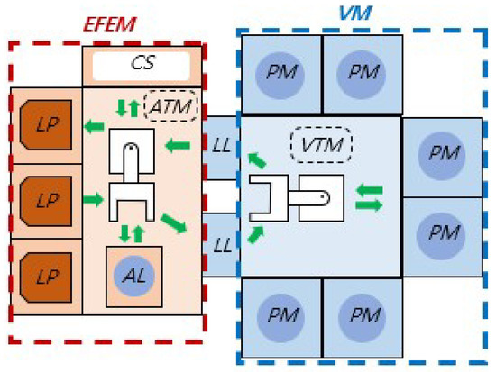
Figure 1.
A typical wafer manufacturing process flow.
There are many previous publications on the method of designing motion profiles. Meckl conducted a study to create an S-curve motion profile that minimizes residual vibration [6]. Kuo classified motion profiles into S-curve, sine curve, and cubic polynomial curve and found an optimal curve that satisfies the minimum motion time [7]. Yang proposed a point-to-point trajectory planning algorithm with a non-linear convex optimization approach for a variable-geometry truss (VGT) manipulator [8]. Huang created a motion profile through the fifth-order B-spline considering the travel time and mean jerk and optimized using a non-dominated sorting genetic algorithm [9]. The place where the semiconductor process is performed is composed of micro- or nano-scale precise processes, and the robot’s motion must also be very accurate. In addition, wafer transfer speeds must also be fast to meet continuous semiconductor production and supply. In a related study, Ni found the optimal traffic category through a polynomial equation when system constraints were given. Lee proposed the optimization method and order selection method of nth-order polynomial motion profile considering transfer time and residual vibration [10]. Aribowo performed trajectory planning using a cubic spline curve to suppress wafer vibration and minimize motion time [11]. Yu used the probability roadmap method (PRM) to consider collision avoidance when transferring wafers to conduct traffic planning through a cubic B-spline curve [12].
In addition, studies on an asymmetric motion profile with different acceleration and deceleration profiles have been actively pursued [13,14,15,16]. Tasy proposed an asymmetrical S-curve motion with fast acceleration and slow deceleration to minimize residual response and settling time in punching machines [13]. Rew designed an S-curve profile that minimized vibration according to long, medium, and short motion distances by adjusting the jerk ratio [14]. Amthor Arvid performed time-optimal asymmetric trajectory planning by extending it to three motion axes [15]. Recently, Wu optimized an S-curve to have a minimum execution time by utilizing point-to-point projection planning (PTPA) as a motion profile of a six-axis industrial robot [16].
Previously, the Bezier curve, a mathematical curve defined by a set of control points, was a curve modification method commonly used in the path-planning research of mobile robots. Song calculated and compared the path planning of the mobile robot using curves such as the Bezier curve, cubic spline curve, and B-spline curve [17]. Jolly studied the path planning of mobile robots for obstacle avoidance in the presence of moving obstacles through the Bezier curve [18]. Choi used the Bezier curve to smooth corner rotation when an autonomous ground vehicle is given waypoints and a corridor [19]. Elhoseny used the Bezier curve with a genetic algorithm to design an optimal path to avoid obstacles and reach the destination [20]. On the other hand, the Bezier curve has yet to be used much in the velocity profile design. Until now, motion profiles have been created using polynomial curves with jerk or acceleration limitation. However, González suggested that designing motion profiles with quintic Bezier curves leads to smoother curves compared to polynomial curves with the jerk limitation method. González created a smooth velocity profile with a quintic Bezier curve, considering the jerk curvature for passenger comfort [21]. Here, travel time was not an optimization factor, and the location of the curve’s control points was limited to the constraints set by the author, so all degrees of freedom were not fully considered. Therefore, we consider the travel time and optimize this by increasing the degree of freedom of the control points. In addition, since optimization was only performed on fifth-order Bezier curves in the past, the difference in the optimization results according to other order curves could not be shown. Therefore, we plan to not only optimize the fifth-order Bézier curve, but also other orders. Furthermore, the acceleration/deceleration section of the velocity profile so far has been designed to be symmetric. Symmetric velocity profiles do not consider changes in robot dynamics during motion. This is because constraints of the velocity profile change according to the change in robot dynamics. Therefore, since the contact conditions between the wafer and the end effector change, especially during motion, we design an asymmetric velocity profile that reflects these changes.
Recognizing the benefits and drawbacks of the previous developments, the present work tries to deliver a control method that could minimize the wafer delivery takt time by a new velocity profile design. Furthermore, it is combined with iterative learning for further reduction in wafer vibrations. In other words, this work shows how to optimize a robot’s velocity profile with a separate dynamics evaluation of the accelerating and decelerating phase of the wafer-carrying robot motion. Furthermore, it also presents a method to apply the designed input to a popular control so that the excessive wafer vibration and slip are significantly reduced.
In Section 2, this work presents the designed profile using the cubic Bezier curve, the lowest order for creating a symmetric velocity profile, and describes the optimization of higher-order Bezier curves by designing profiles using quintic Bezier curves. In Section 3, the calculated profiles are given to a wafer transport robot to compare the wafer transfer efficiency. Section 4 shows the proposed motion profile design considering robot dynamics with iterative learning control (ILC). ILC is a feed-forward control technique that uses previous error information and creates an optimal input profile by repeated learning based on the error between the desired and actual profiles [22,23].
2. Velocity Profile Design
2.1. Cubic Bezier Curve
The nth degree of the Bezier curve can be described in the form of Bernstein polynomials [24]. This work used the Bezier curve to formulate a velocity profile. The nth degree of the Bezier curve equation:
In Equations (1) and (2), t is the position where the space from 0 to 1 m where the curve is drawn, is divided into regular intervals. Therefore, it is a variable that draws a Bezier curve in an arbitrary space between 0 and 1, regardless of the time variable of the actual velocity profile. Furthermore, is the coordinate of the control points that determine the shape of the curve.
The motion profile to be designed was determined to generate a linear motion on the horizontal surface, which is required for loading and unloading wafers, and a rotational motion, which moves wafers in different directions. First, this work modified the velocity profile with a cubic Bezier curve. The transportation distance was determined to match the robot workspace radius and the actual process. The rectilinear motion was 680 mm, and the rotational motion was .
This work assumes that the robot’s motion starts from complete rest and stops at complete rest. Therefore, four conditions that satisfy the assumption should be clarified. The first condition is that the starting and finishing point velocity is zero. Second, the start and final points of the overall profile have zero acceleration. Third, the whole profile is symmetrical for half the total working time. Therefore, the profiles of acceleration and deceleration section are symmetrical. This means that once the acceleration profile is designed, the constant velocity and deceleration section profiles are automatically calculated. That is, it has local control capability for the entire section of the acceleration section. Last, it is assumed that the shape of the acceleration and deceleration profiles are point-symmetric for the centre point for the symmetrical profile design. Therefore, before designing the asymmetric profile, the symmetric profile is first optimized. This will be used for the asymmetric profile design. As a result, the entire profile can be optimized by only calculating the acceleration interval. Since the acceleration and deceleration sections are designed as control points for creating a Bezier curve, the computational complexity of the optimization process increases as the order of the Bezier curve increases. Since the profile of the acceleration interval is point-symmetric, the odd-order Bezier curve would be a good choice. The even-order Bezier curve is not point-symmetric or creates a profile with an unnecessary additional order.
2.1.1. Objective Functions
We used two different objective functions to reduce the transfer time and wafer residual vibration. One used the formula to calculate the total time of the profile to minimize the transfer time, and the other used the formula to calculate the jerk magnitude to consider the residual vibration of the wafer. Therefore, to reduce the transfer time and wafer vibration, different objectives were set up to control wafer transfer and vibration. Three design variables for optimization are considered in the present work. The first variable is the acceleration time. The second variable is the maximum velocity. The third is the control point ratio. A cubic Bezier curve consists of four control points. Each control , , , and , corresponds to the x-coordinate of and corresponds to the y-coordinate of . Therefore, is the ratio of the x-coordinate of to the x-coordinate of .
First, the created velocity profile should minimize the transfer time. Since the calculation of the symmetrical Bezier profile area is the same as calculating the area of a trapezoidal profile, this work obtains the transfer time by dividing the velocity profile area by the maximum velocity value. The transfer time is
where S is the total travel distance.
The second goal is to transfer wafers as accurately as possible. The vibration generated by the wafer affects the wafer transfer accuracy. Furthermore, the vibration is affected by the jerk of the motion profile. Therefore, the jerk of the profile should be kept at a minimum [6,7,9,10,11,14]. This work obtains the magnitude of the maximum jerk by solving the point where the value becomes zero in the jerk derivative. In Equation (1) of the velocity profile, the maximum jerk is in the interval because the acceleration and deceleration intervals are divided based on . The Jerk derivative can be calculated by differentiating the velocity profile equation using the chain rule. The maximum jerk is
2.1.2. Constraints
When designing the velocity profile, the first constraint is the fixed transfer distance. The area of the velocity profile is the same as the total transfer distance. A constraint condition related to the transfer distance is
The wafer should not slip on the end effector while the robot is in motion. Therefore, the maximum acceleration of the wafer should be less than the acceleration that pushes the wafer to slide. The maximum acceleration () using the coefficient of maximum static frictional force is obtained experimentally. The safety factor is 1.2 to account for the distributions of the experiment. The experiment was conducted eight times in total. The maximum static friction coefficient was calculated by placing the wafer on the end effector and tilting it in various directions through the angle at which the wafer starts to slide. We used the average value of the calculated results. The actual maximum static friction coefficient may vary each time depending on various factors such as non-uniform surface roughness, sliding direction or the influence of foreign substances. However, it was unreasonable to reflect this in the constraints of designing the velocity profile every time. Therefore, in this paper, it is assumed that the maximum static friction coefficient is constant by using the average value. The designed profile has a symmetrical shape that has maximum acceleration when t is 0.5. The maximum acceleration is
Since the bounds for the design variable should be greater than the motor’s time constant () when the rotation of the motor reaches maximum velocity, the upper boundary of should be the maximum velocity of the profiles. The maximum velocity was calculated by considering the motor maximum rotational speed and the robot forward kinematics. The lower boundary used the minimum velocity the profile could have under the maximum acceleration time condition. Finally, the bounds of were set considering the conditions under which Equation (4) would have a real number. The variable range is
2.2. Quintic Bezier Curve
Although the quintic Bezier curve profile could be acquired by the same method used in the cubic Bezier, it might be challenging to obtain the maximum jerk in this way. Since there are more variables to be considered, its computation is sometimes prohibitive. Consequently, the response surface method (RSM) was preferred to calculate the maximum jerk in this work. In addition, the optimization of the nth-order Bezier curve is carried out by obtaining the maximum jerk in this way.
2.2.1. Response Surface Methodology
The quintic Bezier curve has two more control points and than the cubic Bezier curve. Two design variables are added to determine the position in the x and y coordinates for one control point because the profile is point-symmetric to the point at . Of the five design variables, and are the same as in the cubic Bezier, while , , and are control point ratios. corresponds to the ratio of the x-coordinate value of to the x-coordinate value of , and corresponds to the ratio of the x-coordinate value of to the x-coordinate value of . corresponds to the ratio of the y-coordinate value of to the y-coordinate value of .
Assume that the maximum jerk of the quintic Bezier curve has a second-order response surface model within a specific region [25]. This is the second-order model of RSM:
Among the factors determining the maximum jerk in the quintic Bezier curve, and determine the horizontal and vertical size of the curve, and , , and determine the shape of the curve. Therefore, since calculating the maximum jerk for any , depends on the values of , , and . Therefore, we established a second-order response model only using , , and .
Experimental factors were determined using central composite design (CCD), widely used in second-order models, to obtain the coefficient of each variable. When the number of factors is three, the CCD places the factors in a combination of eight corners, six centres, and six axial points [25]. The factors’ interest area was set to have no extreme value by referring to the range where control point ratios were calculated in the cubic Beizer profile. , which determines the position of axial points, was set to 1.4 so that it did not deviate significantly from the interest area. Each variable range was normalized to exist between −1 and 1. After this, twenty results were acquired by applying CCD. Each experimental factor produces a different Bezier curve. To obtain the maximum jerk value, the jerk curve was first calculated through differentiation. When the range from 0 to 1 of t was divided by 0.01 intervals and substituted into the jerk equation, the largest jerk value was obtained through the MATLAB program. Table 1 shows the results according to the experimental factors.

Table 1.
List of experimental factors.
2.2.2. Analysis of Variance
After obtaining the regression equation through RSM using Table 1, this work utilized an analysis of variance (ANOVA) to verify reliability [25]. The initial RSM equation is
In the ANOVA of Equation (9), this work evaluated the model fit through the coefficient of determination () [25]. It observed the adjusted and predicted it to compensate for the next . In addition, when both values are not high enough, it is highly possible to be overfitted. Furthermore, eliminating the insignificant error terms in the regression model is necessary. To find the insignificant terms, standardized effect, F-value, and p value for each term of the Pareto chart are calculated with reliability of 95%
By pooling the error terms sequentially from the least significant terms, the model with the highest fit becomes Equation (10). If more terms were pooled, the coefficient of determination was rather reduced. Shown in Table 2, the predicted of the final model was raised to 71.55%, and this work concluded that the adjusted is also a reliable level for the regression model, still showing a value above 90%. Shown also in Figure 2 and Table 3 and Table 4, it is possible to observe how effective each term of the first and last models are in the results. Therefore, Equation (10) is used as an expression for the maximum jerk of the quintic Bezier curve. The higher order of the Bezier curve by the regression equation for the maximum jerk can be optimized. This is the final RSM equation:
Table 2.
Coefficient of determination.
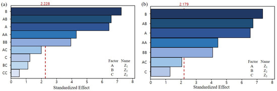
Figure 2.
Pareto chart: (a) Initial model; (b) final model.
Table 3.
ANOVA of initial response surface model.
Table 4.
ANOVA of final response surface model.
Constraint conditions were set for travel time and maximum acceleration in the same way as the cubic Bezier curve’s constraint conditions. However, the bounds of the design variables were determined by considering set by CCD. The variable range is
2.3. Genetic Algorithm Bezier Curve
The genetic algorithm is one of the most popular methods for optimizing multi-objective functions. The objective functions of the cubic Bezier curve optimization process are Equations (3) and (4), the constraints are Equations (5) and (6), and the range of the design variables is Equation (7). The objective function of the quintic Bezier curve optimization process is Equations (3) and (10), the constraints are Equations (5) and (6), and the range of the design variables is Equation (11). Optimization was performed by limiting the range of design variables in order not to calculate an infeasible solution. The optimization results are presented with a distribution diagram through the objective function space, as shown in Figure 3. Since both the cubic and quintic Bezier curves show convex curves, it can be inferred that the optimization could be achieved relatively straightforwardly.
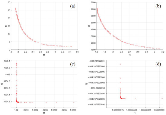
Figure 3.
Pareto front: (a) Rotational motion of the cubic Bezier, (b) linear motion of the cubic Bezier, (c) rotational motion of quintic Bezier, and (d) linear motion of quintic Bezier.
Among Pareto sets, it is impossible to find an optimal single solution that can satisfy all objectives at the same time due to the trade-off relationship between the objective functions. The optimum points in every Pareto set are equal levels of solution. Nevertheless, it is generally desirable to obtain a point as a solution [26]. The most commonly used method for obtaining a single point is to draw the boundary line L(, ) at extreme points and in the Pareto front. The Pareto-optimal point () is the point with maximum distance with this straight line [27]. The Pareto-optimal point is called the knee point, and the knee point was obtained from both the cubic and quinic Bezier curves. However, since the Pareto front obtained through the quintic Bezier curve contains a weak Pareto front, the knee point was calculated by only considering the strict Pareto front [28]. Table 5 shows the parameter information of the final Bezier profiles.
Table 5.
Information of the optimal Bezier profile.
3. Experiment
3.1. Experimental Setup
A wafer transfer robot was used to measure the transfer accuracy of the optimized velocity profiles. The experimental equipment consists of one axis rotating the robot body and another moving the robot arm linearly. The robot continuously operates the rotational motion of the robot body and the linear motion of extending the robot arm to transfer the wafer. The motor was powered by Yaskawa’s servo motor and a reducer to the robot arm. The upper controller was NI’s CompactRIO, and the robot was controlled using the Labview software in a window environment. Figure 4 schematically shows the configured robot system.
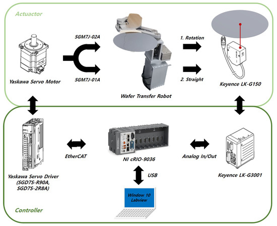
Figure 4.
Schematic diagram of the wafer transfer robot.
The wafer transfer robot moves wafers from one chamber to another. The wafer enclosure used was a front opening unified pod (FOUP) device. The wafer is densely loaded in the vertical direction in the FOUP. Therefore, positional precision in the vertical direction is crucial to avoid other wafer positions during wafer transfer. Therefore, the experiment was conducted by measuring the gravitational vibration immediately after the end of the wafer transfer. Wafer motion and vibration were measured using a laser displacement sensor Keyence LK-G150 and LK-G3001 for the controller.
3.2. Experimental Results
The conventional S-curve is a second-degree polynomial velocity profile with trapezoidal acceleration. The conventional S-curve was selected as the velocity profile to be compared with optimized Bezier profiles in a comparative study. For a fair comparison, the transfer time and maximum velocity of the comparative group S-curve trapezoidal profiles were designed to be the same as the Bezier profiles.
Velocity profiles were given to the robot, and a control loop was constructed using a P control that received feedback from the encoder value of the motor. Then, the vibration of the wafer was measured immediately after the desired robot motion ended. Vibrations at the tip and centre were measured. Settling time was defined when the vibration amplitude converged below ±50 μm. The experiment was conducted with ten repetitions per profile, and the average settling time was calculated and compared. The results are provided in Table 6. The test results confirm that the designed quintic Bezier profile provides the best performance.
Table 6.
Test results.
In addition, data were observed for 500 ms to calculate the energy of the wafer during the settling time. After connecting all experimental data to increase the frequency resolution, the Hann window was applied to remove the effect on the discontinuity of the data [29]. Since the time length of one experimental data was 500 ms, a Hann window of 500 ms was applied. When 10 sets of experimental data were concatenated using a window function followed by FFT, a natural frequency that gradually decreases from 2 Hz is generated. However, the desired frequency domain was the energy size around 10 Hz, and the 2 Hz natural frequency component was smaller than the main frequency component, as show in Figure 4, so the effect was insignificant. We were able to reduce the FFT frequency interval from 2 Hz to 0.2 Hz through the Hann window. Data in the time domain were converted to the frequency domain via a fast Fourier transform (FFT), and then the energy was calculated by the square of the magnitude. Figure 5 shows the energy size in the frequency domain for vibration data immediately after the end of the motion. This confirmed that the Beizer profile required less energy than the comparative S-curve group in a similar frequency area.
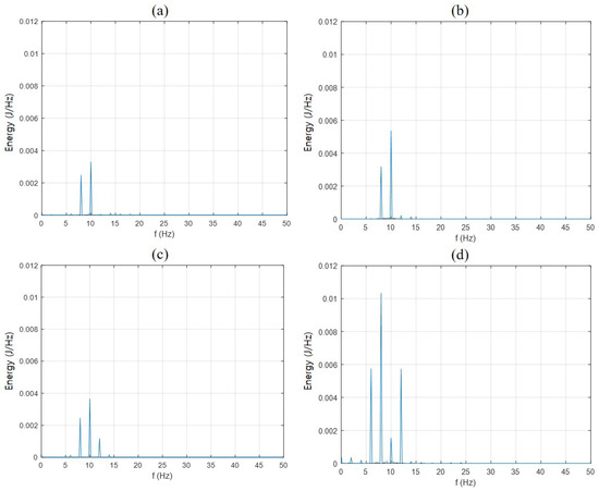
Figure 5.
Residual vibration: (a) Cubic Bezier, (b) S-curve trapezoid 3, (c) quintic Bezier and (d) S-curve trapezoid 5.
3.2.1. Robot and End Effector Vibration
Before the performance comparison between the profiles, a modal test was carried out to identify the natural frequencies of the robot that the velocity profile should avoid. The average robot’s vibration characteristics were identified through ten experiments. The left graph of Figure 6 is the vibration data for the time domain for ten impacts. The right graph is a FFT result of the vibration data. The graph shows that the natural frequency of the robot is near 12 Hz. In particular, the most significant frequency value was 12.1 Hz. The next most significant value was 11.9 Hz. The noise effect of the sensor determined the frequency value existing in the low-frequency band near 0 Hz. The reason for this is that the frequency domain of the robot immediately after the end of the motion, shown in Figure 5, is relatively small in the low-frequency domain.
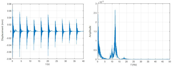
Figure 6.
Modal test result: (a) Vertical vibration in the time domain and (b) in the frequency domain.
3.2.2. Energy Spectrum
Profiles were observed in the frequency domain to determine the cause of the settling time difference between the Bezier and comparison profiles. Figure 7 shows the results of the energy spectrum according to the frequency domain on a log scale of the profiles. Considering that the natural frequency of the robot was around 12 Hz, the amount of energy in the frequency domain of about 11.5∼12.5 Hz was calculated by the Riemann sum. As a result, as can be seen from Table 7, it was confirmed that the Bezier profile has a smaller amount of energy in linear motion than its comparison counterpart. On the other hand, in rotational motion, the difference in the amount of energy was insignificant. Even in the rotational motion of the cubic Bezier profile and its comparison profile, the comparison profile had less energy in total. However, it did not significantly impact the robot’s residual vibration since the rotational motion happened before the linear motion. Additionally, the amount of energy was less than in linear motions.
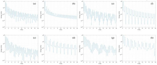
Figure 7.
Log scale energy spectrum of input profiles: (a) Rotational and (b) linear cubic Bezier, (c) rotational and (d) linear quintic Bezier, and (e–h) comparison profiles of (a–d).
Table 7.
Energy 1 of the input profiles in the frequency 2 domain.
Comparing the cubic and quintic Bezier profiles in linear motion, despite that the sum of energy at 11.9∼12.1 Hz was more significant in the quintic Bezier, the settling time was better than the cubic Bezier. Note that the frequency with the largest amplitude was 12.1 Hz, and at that frequency the linear motion’s quinic Bezier profile has about 100 times less energy than the cubic.
4. Asymmetric Profile
4.1. Friction
The quintic Bezier profile performed better than the cubic for the settling time. However, there is another issue with accurate wafer transportation. In an accelerating robot and end effector motion, the wafer often slips on an end effector, which results in wafer re-centring costs. Although wafer slippage can occur for various reasons, the deflection of the end effector in the direction of gravity caused by the weight of the robot might be one of the primary sources of the slip motion since the deflection might change the friction conditions. As a result, this work focused on the effect of the deflection of the end effector. A simulation model of the end effector before and after the acceleration or deceleration was constructed. As shown in Table 8, different deflection angles were obtained depending on the profile sections, and the deflection angle after deceleration was approximately double before acceleration.
Table 8.
Deflection angle at the end effector before acceleration and after deceleration.
The friction model between the end effector and the wafer and the threshold acceleration at which the slip begins was calculated. Figure 8 is a schematic friction model that defines the forces acting on wafers before and after acceleration. Coulomb friction is adopted without loss of generality for this wafer and the end effector contact [30]. In addition, drag force acting in the opposite direction in accelerating and decelerating situations was also considered as the aspect ratio of the wafer geometry is unique. Therefore, the effect of the airlift or compressive force on the entire friction seems worth considering.
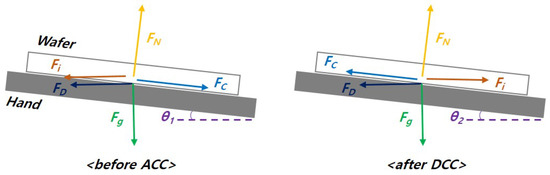
Figure 8.
Friction model between the wafer and end effector.
is the weight of the wafer, is the normal force, is the friction force, is the drag force, and is the inertial force. Considering that the summation of the forces acting on the wafer is zero for vertical and horizontal axes, the acceleration at which the slip begins to occur can be determined. Equations (12) and (13) are accelerations for the acceleration and deceleration slips, respectively. m is the mass of the wafer and g is the gravitational acceleration.
The model confirms that the threshold acceleration for slippage is different from the decelerating situation by about 20 mm/s. Consequently, the slippage monitored during deceleration with the quintic Bezier happened due to the deflection which changed the frictional situation between the wafer and the end effector.
To prevent the slip, either increasing the friction or decreasing the deceleration should be selected. However, since re-designing the robot and end effector for less deflection would be prohibitively expensive, the option normally available is re-designing the deceleration profile.
4.2. Quintic–Cubic Bezier Profile
The Pareto front of Figure 3b, obtained as an optimal result of the cubic Bezier, was utilized to redesign the deceleration section of the quintic Bezier profile. Because all solutions in the Pareto front are optimized, a cubic Bezier profile with the same maximum velocity as the quintic Beizer is the best option. As a result, parameters of the optimal quintic–cubic Beizer asymmetric velocity profile are listed in Table 9 and depicted in Figure 9a. The newly obtained velocity profile was given to the robot under the same conditions as the previous experiments. The average settling time of the ten tests was 236 ms, significantly less than the previous cases shown in Table 6. In addition, Figure 9b can be compared with Figure 5 for the vibration level, confirming the outstanding performance of the suggested asymmetric profile. Note that the scale of Figure 9b y-axis is .
Table 9.
Information of the optimal quintic–cubic Bezier profile in linear motion.
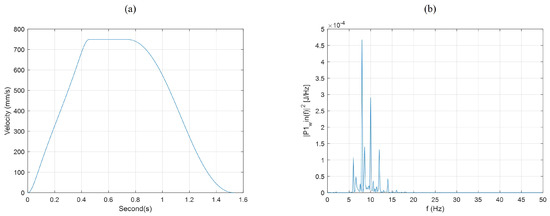
Figure 9.
Designed asymmetric velocity profile and residual vibration. (a) The optimal quintic-cubic Bezier asymmetric velocity profile, (b) Energy spectrum.
5. Asymmetric Velocity Profile with Iterative Learning Control
In this section, to maximize the efficacy of the presented method that reduces wafer slippage and residual vibration, an advanced control method is applied for the overall takt time reduction. Iterative learning control (ILC), actively used for systems where a repetitive task is required, such as wafer transferring tasks, is a good candidate. First, to apply ILC, an error in the time domain between the input profile and the motor encoder values was obtained. In this work, the data were converted to the frequency domain and multiplied by the learning gain to obtain the frequency domain error. The updated error changed the specific frequency component of the desired profile. After this, a new input profile was created by converting it back into the time domain [31,32]. The input update law is
Then, iteration was carried out to minimize the value by defining the difference between the position per time of the input profile and the encoder value of the real-time motor as a cost function. This way, the error was more effectively converged. Figure 10 shows the error behaviour of the Bezier profiles during repetitive learning. With five iterations, the input profiles were able to be created.
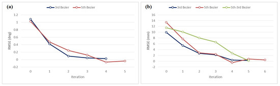
Figure 10.
Tracking error during iterative learning: (a) Rotational motion and (b) linear motion.
The experiment was conducted with the optimal cubic–quintic Bezier profile to estimate wafer transfer accuracy under the same robot test conditions. Figure 11 shows the residual vibration of the cubic, quintic, and quintic–cubic Bezier profiles with ILC. The two horizontal lines in a1, b1, and c1 of Figure 11 mean the vibration amplitude of ±50 μm used when defining the settling time. The test confirms the superior wafer handling performance of the presented control method, combining the optimized quintic–cubic Bezier profile and the frequency domain ILC. Figure 12 shows a summary of the settling times of all profiles presented in this work.
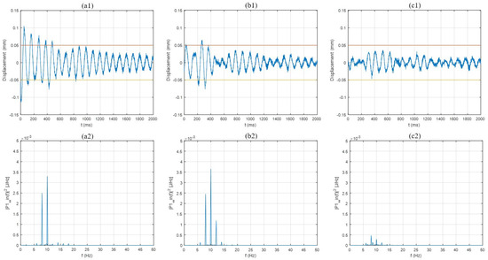
Figure 11.
Residual vibrations: (a) Cubic Bezier with ILC, (b) Quintic Bezier and (c) quintic–cubic Bezier.
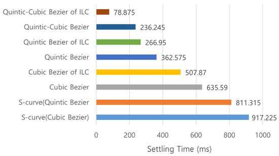
Figure 12.
Average settling time comparison.
6. Discussion
In most previous research, the curves used for velocity motion were splines modified based on the polynomial Equation [10,11,12,33]. Unlike previous work, the Bezier curve used in this paper showed the advantage of creating a smooth jerk profile even with low order. In addition, it is confirmed that the shorter the wafer travel time, the more effectively the Bezier curve increased the transfer accuracy. Furthermore, this work showed the optimization process to acquire the necessary profiles. Mechanical models for slip conditions between wafers and the end effector were formulated to minimize wafer slippage. Furthermore, an asymmetric profile with different acceleration and deceleration was designed. Although there were many asymmetric motion profiles studied with S-curves [13,14,15,16], this work adopted the asymmetric motion profile with the Beizer curve and experimentally compared the symmetric Bezier profile with wafer transfer accuracy. Combined with the frequency domain ILC, the asymmetric Beizer curve provides a notable improvement in the accuracy and settling time for the wafer transfer robot operation that can reduce the overall takt time in semiconductor production.
Author Contributions
Conceptualization, K.S.Y. and J.C.K.; methodology, K.S.Y. and J.C.K.; software, K.S.Y.; validation, K.S.Y. and J.C.K.; formal analysis, K.S.Y.; investigation, K.S.Y.; resources, K.S.Y., M.S.K., H.M. and H.R.C.; data curation, K.S.Y.; writing—original draft preparation, K.S.Y.; writing—review and editing, M.S.K. and J.C.K.; supervision, J.C.K. All authors have read and agreed to the published version of the manuscript.
Funding
This work was supported by the National Research Foundation of Korea (NRF) grant funded by the Korea government (MSIT) (No. NRF-RS-2023-00209266).
Institutional Review Board Statement
Not applicable.
Informed Consent Statement
Not applicable.
Data Availability Statement
Not applicable.
Conflicts of Interest
The authors declare no conflict of interest.
References
- Cha, J.; Park, J.; Jeong, J. A Novel Defect Classification Scheme Based on Convolutional Autoencoder with Skip Connection in Semiconductor Manufacturing. In Proceedings of the 2022 24th International Conference on Advanced Communication Technology (ICACT), Pyeongchang, Republic of Korea, 13–16 February 2022; pp. 347–352. [Google Scholar]
- Hong, C.; Lee, T.-E. Modeling, Simulation and Supervisory Control of Semiconductor Manufacturing Cluster Tools with an Equipment Front-End Module. In Proceedings of the 2020 IEEE 16th International Conference on Automation Science and Engineering (CASE), Hong Kong, China, 20–21 August 2020; pp. 703–709. [Google Scholar]
- Wang, H.; Wang, H.-G.; Xu, W.-L. Cyclic scheduling of cluster tools with equipment front-end module and multifunctional load locks. In Proceedings of the 26th Chinese Control and Decision Conference (CCDC), Changsha, China, 31 May–2 June 2014; pp. 4448–4453. [Google Scholar]
- Zhu, Q.; Wang, G.; Hou, Y.; Wu, N.; Qiao, Y. Optimally Scheduling Dual-Arm Multi-Cluster Tools to Process Two Wafer Types. IEEE Robot. Autom. Lett. 2022, 7, 5920–5927. [Google Scholar] [CrossRef]
- Ko, S.-G.; Yu, T.-S.; Lee, T.-E. Scheduling dual-armed cluster tools for concurrent processing of multiple wafer types with identical job flows. IEEE Trans. Autom. Sci. Eng. 2018, 16, 1058–1070. [Google Scholar] [CrossRef]
- Meckl, P.H.; Arestides, P.B. Optimized s-curve motion profiles for minimum residual vibration. In Proceedings of the 1998 American Control Conference, ACC (IEEE Cat. No. 98CH36207), Philadelphia, PA, USA, 26 June 1998; pp. 2627–2631. [Google Scholar]
- Kuo, Y.-L.; Lin, C.-C.; Lin, Z.-T. Dual-optimization trajectory planning based on parametric curves for a robot manipulator. Int. J. Adv. Robot. Syst. 2020, 17, 1729881420920046. [Google Scholar] [CrossRef]
- Yang, Y.; Jiang, B.; Hu, S. Fast trajectory planning for VGT manipulator via convex optimization. Int. J. Adv. Robot. Syst. 2015, 12, 136. [Google Scholar] [CrossRef]
- Huang, J.; Hu, P.; Wu, K.; Zeng, M. Optimal time-jerk trajectory planning for industrial robots. Mech. Mach. Theory 2018, 121, 530–544. [Google Scholar] [CrossRef]
- Lee, D.; Ha, C.-W. Optimization process for polynomial motion profiles to achieve fast movement with low vibration. IEEE Trans. Control. Syst. Technol. 2020, 28, 1892–1901. [Google Scholar] [CrossRef]
- Aribowo, W.; Terashima, K. Cubic spline trajectory planning and vibration suppression of semiconductor wafer transfer robot arm. Int. J. Autom. Technol. 2014, 8, 265–274. [Google Scholar] [CrossRef]
- Yu, X.; Zhao, Y.; Wang, C.; Tomizuka, M. Trajectory planning for robot manipulators considering kinematic constraints using probabilistic roadmap approach. J. Dyn. Syst. Meas. Control 2017, 139, 021001. [Google Scholar] [CrossRef]
- Tsay, D.-M.; Lin, C.-F. Asymmetrical inputs for minimizing residual response. In Proceedings of the IEEE International Conference on Mechatronics, 2005. ICM, Taipei, Taiwan, 10–12 July 2005; pp. 235–240. [Google Scholar]
- Rew, K.-H.; Kim, K.-S. A closed-form solution to asymmetric motion profile allowing acceleration manipulation. IEEE Trans. Ind. Electron. 2009, 57, 2499–2506. [Google Scholar] [CrossRef]
- Amthor, A.; Werner, J.; Lorenz, A.; Zschäck, S.; Ament, C. Asymmetric motion profile planning for nanopositioning and nanomeasuring machines. Proc. Inst. Mech. Eng. Part I J. Syst. Control Eng. 2010, 224, 79–92. [Google Scholar] [CrossRef]
- Wu, Z.; Chen, J.; Bao, T.; Wang, J.; Zhang, L.; Xu, F. A Novel Point-to-Point Trajectory Planning Algorithm for Industrial Robots Based on a Locally Asymmetrical Jerk Motion Profile. Processes 2022, 10, 728. [Google Scholar] [CrossRef]
- Song, B.; Tian, G.; Zhou, F. A comparison study on path smoothing algorithms for laser robot navigated mobile robot path planning in intelligent space. J. Inf. Comput. Sci. 2010, 7, 2943–2950. [Google Scholar]
- Jolly, K.G.; Kumar, R.S.; Vijayakumar, R. A Bezier curve based path planning in a multi-agent robot soccer system without violating the acceleration limits. Robot. Auton. Syst. 2009, 57, 23–33. [Google Scholar] [CrossRef]
- Choi, J.-W.; Curry, R.; Elkaim, G. Path planning based on bézier curve for autonomous ground vehicles. In Proceedings of the Advances in Electrical and Electronics Engineering-IAENG Special Edition of the World Congress on Engineering and Computer Science, San Francisco, CA, USA, 22–24 October 2008; pp. 158–166. [Google Scholar]
- Elhoseny, M.; Tharwat, A.; Hassanien, A.E. Bezier curve based path planning in a dynamic field using modified genetic algorithm. J. Comput. Sci. 2018, 25, 339–350. [Google Scholar] [CrossRef]
- González, D.; Milanés, V.; Pérez, J.; Nashashibi, F. Speed profile generation based on quintic Bézier curves for enhanced passenger comfort. In Proceedings of the 2016 IEEE 19th International Conference on Intelligent Transportation Systems (ITSC), Rio de Janeiro, Brazil, 1–4 November 2016; pp. 814–819. [Google Scholar]
- Mishra, S.; Tomizuka, M. Projection-based iterative learning control for wafer scanner systems. IEEE/ASME Trans. Mechatron. 2009, 14, 388–393. [Google Scholar] [CrossRef]
- Oh, D.J.; Baek, S.G.; Nam, K.-T.; Koo, J.C. Tracking and Synchronization with Inversion-Based ILC for a Multi-Actuator-Driven Wafer Inspection Cartridge Transport Robot System. Electronics 2021, 10, 2904. [Google Scholar] [CrossRef]
- Prautzsch, H.; Boehm, W.; Paluszny, M. Bézier and B-Spline Techniques; Springer: Berlin/Heidelberg, Germany, 2002; pp. 9–13. [Google Scholar]
- Myers, R.H.; Montgomery, D.C.; Anderson-Cook, C.M. Response Surface Methodology: Process and Product Optimization Using Designed Experiments, 4th ed.; John Wiley & Sons: Hoboken, NJ, USA, 2016. [Google Scholar]
- Miettinen, K. Nonlinear Multiobjective Optimization; Springer Science & Business Media: Berlin/Heidelberg, Germany, 2012; pp. 10–17. [Google Scholar]
- Deb, K.; Gupta, S. Understanding knee points in bicriteria problems and their implications as preferred solution principles. Eng. Optim. 2011, 43, 1175–1204. [Google Scholar] [CrossRef]
- Coello, C.A.C.; Lamont, G.B.; Van Veldhuizen, D.A. Evolutionary Algorithms for Solving Multi-Objective Problems, 2nd ed.; Springer: Berlin/Heidelberg, Germany, 2007; pp. 10–13. [Google Scholar]
- Prabhu, K.M.M. Window Functions and Their Applications in Signal Processing; Taylor & Francis: Abingdon, UK, 2014; pp. 91–94. [Google Scholar]
- Olsson, H.; Åström, K.J.; De Wit, C.C.; Gäfvert, M.; Lischinsky, P. Friction models and friction compensation. Eur. J. Control 1998, 4, 176–195. [Google Scholar] [CrossRef]
- Bristow, D.A.; Tharayil, M.; Alleyne, A.G. A survey of iterative learning control. IEEE Control Syst. Mag. 2006, 26, 96–114. [Google Scholar]
- Moore, K.L. Iterative Learning Control for Deterministic Systems; Springer Science & Business Media: Berlin/Heidelberg, Germany, 2012. [Google Scholar]
- Ni, Y.; Luo, F.; Zhong, X.; Guo, L. Trajectory Planning of a Parallel Robot for Wafer Transfer. In Proceedings of the 2010 International Conference on E-Product E-Service and E-Entertainment, Henan, China, 7–9 November 2010; pp. 1–4. [Google Scholar]
Disclaimer/Publisher’s Note: The statements, opinions and data contained in all publications are solely those of the individual author(s) and contributor(s) and not of MDPI and/or the editor(s). MDPI and/or the editor(s) disclaim responsibility for any injury to people or property resulting from any ideas, methods, instructions or products referred to in the content. |
© 2023 by the authors. Licensee MDPI, Basel, Switzerland. This article is an open access article distributed under the terms and conditions of the Creative Commons Attribution (CC BY) license (https://creativecommons.org/licenses/by/4.0/).