Long Short-Term Fusion Spatial-Temporal Graph Convolutional Networks for Traffic Flow Forecasting

Abstract

Traffic flow forecasting, as one of the important components of intelligent transport systems (ITS), plays an indispensable role in a wide range of applications such as traffic management and city planning. However, complex spatial dependencies and dynamic changes in temporal patterns exist between different routes, and obtaining as many spatial-temporal features and dependencies as possible from node data has been a challenging task in traffic flow prediction. Current approaches typically use independent modules to treat temporal and spatial correlations separately without synchronously capturing such spatial-temporal correlations, or focus only on local spatial-temporal dependencies, thereby ignoring the implied long-term spatial-temporal periodicity. With this in mind, this paper proposes a long-term spatial-temporal graph convolutional fusion network (LSTFGCN) for traffic flow prediction modeling. First, we designed a synchronous spatial-temporal feature capture module, which can fruitfully extract the complex local spatial-temporal dependence of nodes. Second, we designed an ordinary differential equation graph convolution (ODEGCN) to capture more long-term spatial-temporal dependence using the spatial-temporal graph convolution of ordinary differential equation. At the same time, by integrating in parallel the ODEGCN, the spatial-temporal graph convolution attention module (GCAM), and the gated convolution module, we can effectively make the model learn more long short-term spatial-temporal dependencies in the processing of spatial-temporal sequences.Our experimental results on multiple public traffic datasets show that our method consistently obtained the optimal performance compared to the other baselines.

1. Introduction

Because traffic flow forecasting has wide-ranging applications in people’s everyday lives, the task of predicting traffic data has been studied extensively by researchers. The ability to accurately predict traffic flow data has the potential to significantly improve the efficiency and safety of people’s traffic journeys, particularly on high-traffic, high-speed freeways, where congestion can severely affect their efficiency; accurate prediction of traffic flow can provide the basis for accurate vehicle scheduling and bus system optimization, which can help alleviate urban traffic congestion and improve urban traffic efficiency, and is crucial to promoting the coordinated development of smart transportation and smart city. Based on accurate traffic flow prediction results, traffic police departments can conduct timely traffic dredging to alleviate the congestion caused by excessive traffic.

With the continued development of deep learning in recent years, the graph neural network (GNN) is being widely used in traffic flow prediction. The GNN is applied to obtain the spatial correlation of traffic networks, whereas the time-series module is used to capture temporal correlation, and graph convolution and temporal convolution were introduced into the model methods and were shown to be effective for spatial-temporal feature extraction. While considerable progress has been made in the incorporation of graph structures into spatial-temporal data prediction models, these models still suffer from a number of shortcomings:

• In earlier studies such as DCRNN [1], STGCN [2] and ASTGCN [3], two independent components were used to capture the temporal and spatial dependencies seperately. In these approaches, only spatial dependencies and temporal correlations are captured directly, without considering both temporal and spatial interaction dependencies, and these complex local spatial-temporal correlations can be captured simultaneously and would be highly effective for spatial-temporal data prediction as adopted by STSGCN [4], as this modeling approach reveals the fundamental way in which spatial-temporal network data can be generated.
• Existing studies of spatial-temporal data prediction fail to capture dependencies between local and global correlations simultaneously. RNN/LSTM-based models such as DCRNN and STGCN are time-consuming because the models are relatively complex and do not parallelize the processing task well, and may fade away or explode when capturing remote sequences [5]. The CNN-based approach requires layers to achieve global correlation of long sequences, and STGCN and GraphWaveNet [6] can lose local information if the rate of expansion is increased. STSGCN proposes a new localized spatio-temporal subgraph that synchronously captures local correlations and is only designed locally, ignoring the global information. The situation of learning only local noise is more severe in the presence of missing data.
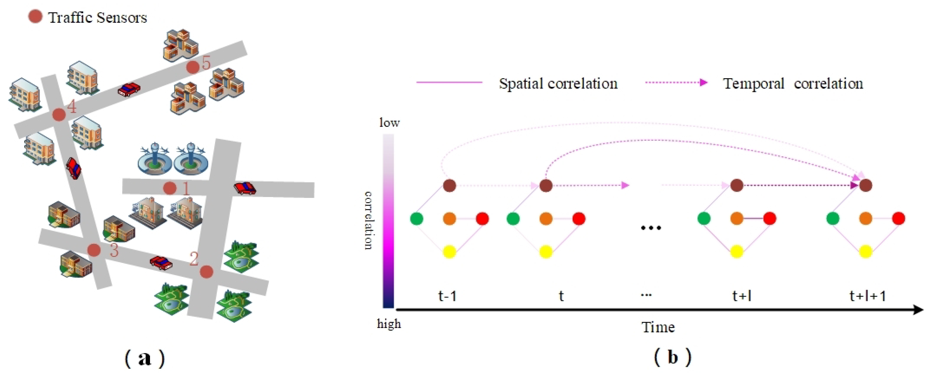
• The traffic flow of a spatial node is not only correlated with the previous time step of the current node, but with the entire history of traffic flow, and this correlation does not become weaker with longer time intervals; in the long run each node’s traffic flow has its own similar temporal “pattern”. As demonstrated in Figure 1a, in an urban transport network, node 1 denotes the station, where the traffic flow during a grand festival such as the Chinese New Year is very variable compared to the previous days, node 3 denotes the school, where the traffic flow on the opening day is quite dissimilar from the summer and winter holidays, and the other nodes often vary greatly in this time “pattern” because of their different locations. Traffic flows in public transport networks are constantly changing dynamically. For many areas of the public transport network, traffic flow at one point in time is closely linked to its historical traffic flow data, which makes long-term traffic flow prediction difficult. As demonstrated in Figure 1b, the color shades of the solid lines between nodes represent the spatial correlation between different roads, while the color shades of the dashed lines represent the temporal influence of historical traffic flow data on the current time point. By learning the short-term and long-term periodicity of historical time series of spatial nodes, the algorithm can better improve the accuracy of traffic flow prediction.

To figure out these challenges, in this paper, we propose a novel deep learning model called long short-term fusion spatial-temporal graph convolutional network (LSTFGCN). The temporal correlation of the traffic in the temporal dimension is first extracted using temporal convolution (TCN). Additionally, in the ordinary differential equations graph convolution (ODEGCN), the wider acceptance domain allows it to capture more dependent features in longer time steps, and the gated convolution is then used to improve the extraction for long term features. The local spatial-temporal convolution attention module is then established to synchronously obtain the local spatial-temporal correlations, and local spatial-temporal features are strengthened using the Convolution Block Attention Module (CBAM) [7]. In conclusion, merging features extracted from different spatial-temporal convolution modules and the gated convolution module can capture more hidden spatial-temporal dependencies in the traffic. LSTFGCN is also capable of using different modules to extract long- and short-term characteristics of a node separately and merge them appropriately to improve the performance of traffic flow forecasting.

We have evaluated LSTFGCN on four public transportation network datasets. The results demonstrate that LSTFGCN can obtain excellent performance. The key contributions of this article are as follows:

• We propose a novel ordinary differential equation graph convolution, which uses the global acceptance domain of a wider graph convolution to learn historical spatial-temporal characteristics by entering historical traffic data of current time step and current time step.
• We propose a novel spatial-temporal graph convolution attention module that can serially generate attentional feature map information in both the channel and spatial dimensions while simultaneously capturing local spatial-temporal correlations, which may be multiplied with previous feature maps for adaptive correction of the features.
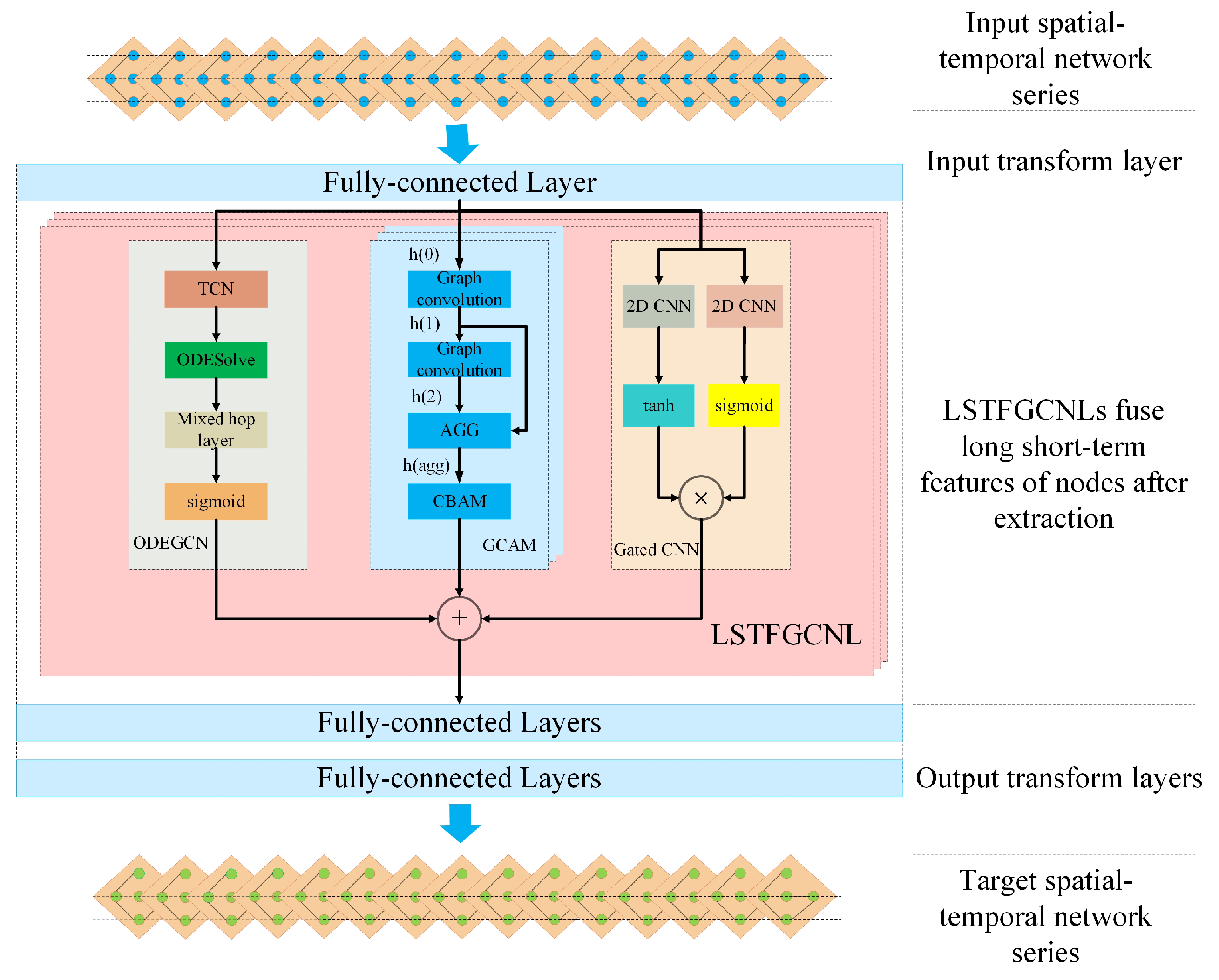
• We propose an efficient framework for capturing both local and global spatial-temporal correlations, and further extract long-range spatial-temporal dependencies by combining a gated extended convolution module with GCAM and ODEGCN in parallel to fuse the long short-term spatial-temporal features of nodes.
• We evaluated our proposed model on four datasets and processed extensive comparison experiments and compared the prediction results with recent model results, demonstrating that the model in this paper achieved better results.

2. Related Work

2.1. Spatial-Temporal Forecasting

Spatial-temporal forecasting plays an important role in many fields of application. In order to more effectively fuse spatial dependencies, recent studies have introduced graph convolutional networks (GCNs) for learning traffic networks. DCRNN models spatial information using bidirectional random wander on the traffic map and captures the temporal dynamics via a gated traffic unit (GRU). Transformers such as those of Wang [8] and Park et al. [9] make use of the spatial and temporal attention modules in the transformer for spatial-temporal modeling. This outperforms LSTM for training, but predictions are still incremental because of its autoregressive structure. STGCN and GraphWaveNet employ graph convolution over the spatial domain as well as one-dimensional convolution along the time axis. These relate to graph and time series information, respectively. STSGCN attempts to fuse spatial-temporal blocks together using a local spatial-temporal convolution graph module, ignoring global interactions.

2.2. Graph Convolutional Network

Graph convolutional networks are used extensively for many graph-based tasks such as classification and clustering [10], of which there are two types. The first is spectral methods, which consider graph convolution locality via spectral analysis, e.g., by finding the corresponding Fourier basis for expanding the convolution in the spectral domain into the graph [11], which was later optimized by Defferrard, Bresson and Vandergheynst [12] using a Chebyshev polynomial approximation in order to implement the eigenvalue decomposition. GCN [13] is representative of work that has built typical baselines in a large number of tasks. A second approach is to use a typical convolution to promote spatial neighborhoods. Spatial methods perform convolutional filtering directly on graph nodes and their neighbors. The heart of this type of method is thus the selection of the neighborhood of nodes. Li et al. [2] introduced graph convolution into the task of recognizing human actions. A number of partitioning strategies have been proposed to partition the neighborhood of each node into different subsets and to guarantee an equal number of subsets for each node. Typical works include GAT [14], which introduces an attention mechanism into the domain of graphs, and GraphSAGE [15], which generates embeddings of nodes through local feature sampling and aggregation.

2.3. Attention Mechanism

Attention mechanisms have been used extensively in recent years in a variety of tasks such as natural language processing, image captioning, and speech recognition. The purpose of the attention mechanism is to select from among all of the inputs information that is relatively critical for the task at hand. Xu et al. [16] proposed two attentional mechanisms in a picture description task and used visualization methods to visualize the effects of attentional mechanisms. In order to classify the nodes of the graph, the self-attentive layer of GAT processes the graph structure data via neural networks and achieves state-of-the-art results. Liang et al. [17] proposed a multi-layer attention network for time series prediction that adaptively adjusts the correlation between the time series of multiple geo sensors. However, it is time-consuming in practice because an independent model needs to be trained for each time series [3]. CBAM is a simple and efficient attention module for convolutional neural networks. It is capable of generating attention feature maps in two dimensions of the channel and feature space, and making adaptive corrections to the original features. Because CBAM is a general purpose end-to-end module, it can be seamlessly integrated into a convolutional layer and can be trained end-to-end with the base convolutional layer.

2.4. Neural Ordinary Differential Equations

The current work typically uses shallow graph convolutional networks and temporal extraction modules to model spatial-temporal dependencies, respectively. Such models, however, have limited representational capabilities: Shallow convolution is unable to capture spatial correlations at a distance, while a larger number of layers can lead to performance degradation in practice [18]. General GNNs have been shown to suffer from problems of over-smoothing. On the basis of earlier work [19,20], Chen et al. [21] proposed a new family of continuous time models, called neural ODEs, which can be interpreted as continuous equivalents of residual networks [22]. The basic neural ODE formulation is given below:

$$\frac{dh\left(t\right)}{dt}=f_{\theta }(h\left(t\right),t),h\left(t_0\right)=h_0,$$

(1)

where $f_{\theta }$ denotes being parameterized as a neural network. The hidden state $h\left(t\right)$ is defined at any time and can be computed at any desired time using the ODE solver as follows:

$$h_0,\dots ,h_T=ODESolve(f_{\theta },h_0,(t_0,\dots ,t_T)),$$

(2)

where T indicates the number of time steps. By using the adjoint method [21], the gradients $\theta$ can be computed memory-efficiently during back propagation.

Recent work [23,24,25,26,27] attempted to analyze this framework theoretically, so as to overcome the instability problem and to improve memory efficiency. Researchers are applying the neural ordinary differential equations to many other fields.

3. Preliminaries

Definition 1. 

Spatial network G. We use $G=(V,E,A)$ to denote the spatial network, where $\left|V\right|=N$ is the set of vertexes, N denotes the number of vertices, E denotes the set of edges, and A is the adjacency matrix of the network G. The spatial network G denotes the relationship of nodes in spatial dimensions and the network structure does not change with time.

Definition 2. 

The graph signal matrix $X_G^{\left(t\right)}\in R^{N\times C}$, where C is the number of attribute features and t is the ${\mathrm{t}}^{\mathrm{th}}$ moment. This graph signal matrix denotes the observed values of the spatial network G at time. The purpose of traffic prediction is to learn the function f from the previous T traffic speed observation and to predict the traffic speed of the next $T^{\prime }$ from the N-related sensors on the road network.

$$[G,X_G^{(t-T+1)},\dots ,X_G^{\left(t\right)}]\stackrel{f}{\to }[X_G^{(t+1)},\dots ,X_G^{(t+T^{\prime })}]$$

where T is the length of the historical spatial-temporal network sequence and $T^{\prime }$ denotes the length of the target spatial-temporal network sequence to be predicted.

4. Model

We show the framework of long short-term fusion spatial-temporal graph convolutional networks in Figure 2. The model is composed of (1) an input layer, (2) a stacked long short-term fusion spatial-temporal graph convolutional network layer (LSTFGCNL), and (3) a layer of output data. The input layer is one fully-connected layer and the output layer is two fully-connected layers, followed by one activation layer such as ReLU [28]. Each LSTFGCNL consists of multiple spatial-temporally parallel graph convolution attention modules, a graph convolution module for ordinary differential equations, and a gated extended convolution module (gated CNN), which contains two parallel extended convolution blocks in two dimensions.

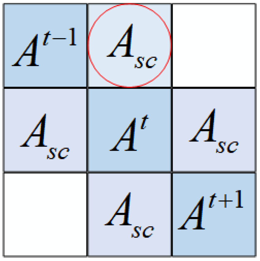
4.1. Localized Spatial-Temporal Graph Construction

As in STSGCN, we constructed a similar model to directly capture each node’s influence on its spatial-temporally adjacent nodes, which are the local node spatial connectivity and temporal correlation between adjacent time steps. In order to achieve synchronous capture of the local time and spatial correlation of the nodes, all nodes must be connected to themselves at adjacent time steps. With each node self-connected at the previous time and at the following time, the result is a local spatial-temporal plot, which directly captures the correlation between each node and its spatial-temporal neighbors.

$A\in R^{N\times N}$ denotes the adjacency matrix of the spatial graph, and N denotes the number of nodes. $A^{\prime }\in R^{3N\times 3N}$ denotes the adjacency matrix of the local spatial-temporal graph built on three continuous time steps. For the node i of $A_i$ in the spatial graph, its new index in the local spatial-temporal graph is calculated by $(t-1)N+i$, where t refers to the number of time steps in the local spatial-temporal graph. If two nodes are connected to each other in this localized spatial-temporal graph, in this case, the corresponding value in the adjacency matrix is set to 1, and in the absence of connectivity, the value is set to 0. The adjacency matrix of the local space-time graph can be expressed as follows:

$$A_{i,j}^{\prime }=\left\{\begin{array}{c}1,if{v}_{i}and{v}_{j}areconnected\hfill \\ 0,otherwise\hfill \end{array}\right.,$$

(3)

where $v_i$ is node i in the local spatial-temporal graph. The adjacency matrix $A^{\prime }$ contains $3N$ nodes. Figure 3 shows the adjacency matrix of the localized spatial-temporal graph. The adjacency matrix $A^{\prime }$ is composed of nine small matrices. The three matrices on the diagonal respectively denote the adjacency matrix $A^{t-1}$ at $t-1$ time and the adjacency matrix $A^t$ and $A^{t+1}$ at t time and $t+1$ time. The $A_{SC}$ matrix on both sides of the diagonal denotes the connectivity between each node and itself in adjacent time slices (unit matrix, namely connectivity is 1). The $A_{SC}$ matrix circled in red in the first row and second column of $A^{\prime }$ in Figure 3 denotes the connectivity of the current node between time step 1 and time step 2 as 1, and the remaining two matrices in the lower left corner and upper right corner are set as 0.

4.2. Spatial-Temporal Graph Convolution Attention Module

The spatial-temporal graph convolution attention module (GCAM) consists of a set of graph convolution and convolutional block attention modules (CBAMs). The graph convolution operation aggregates the features of each node with its neighboring nodes, while the CBAM can make adaptive corrections to the obtained node features. The constructed local spatial-temporal graph is used as the input of GCAM, so that each node can aggregate its own features and those of neighboring nodes at adjacent time steps to achieve the effect of simultaneous extraction of short-term local spatial-temporal features of each node. We also added self-connection at each node of the local spatial-temporal graph, which allows the graph convolution operation to take into account its own characteristics when aggregating features from neighbor nodes. The stacking of multiple graph convolution operations to expand the aggregation region and the increase in the domain of acceptance of graph convolution operations helps to capture local spatial-temporal correlations. A clustering function is a linear combination with weights equal to node weights and edges between adjacent nodes. We then use a fully-connected layer with a chosen GLU [29] activation function, and this graph convolution operation can be formulated as follows:

$$h^{\left(l\right)}=(A^{\prime }{h}^{(l-1)}{W}_1+b_1)\otimes \sigma (A^{\prime }{h}^{(l-1)}{W}_2+b_2),$$

(4)

where $A^{\prime }\in R^{3N\times 3N}$ denotes the adjacency matrix of the local spatio-temporal graph. $h^{(l-1)}\in R^{3N\times C}$ denotes the input to the convolution of the graph of the l layer; when $l=0$, it denotes the initial input. $W_1\in R^{C\times C^{\prime }}$, $W_2\in R^{C\times C^{\prime }}$, $b_1\in R^{C^{\prime }}$, $b_2\in R^{C^{\prime }}$ are learnable parameters, C denotes the number of attribute features, and $C^{\prime }$ denotes the number of features output from the first fully connected layer. ⊗ denotes an element-wise product, and $\sigma (·)$ denotes a sigmoid function.

Then, a new aggregation layer (AGG) was designed to filter the useless information. For GCAM with l layers of graph convolution operations, the output of each graph convolution operation will be fed to the aggregation layer. The aggregation layer will compress all of the outputs in the graph convolution layer. The aggregation operation has two steps: aggregating and cropping.

• Aggregating operation: We chose maximum pooling as the aggregation operation. This algorithm applies a maximum element-wise operation to the output of all graph convolutions in GCAM. The maximal aggregation operation may be expressed as:

  $$h_{agg}=max(h^{\left(1\right)},h^{\left(2\right)},\dots ,h^{\left(l\right)})\in R^{3N\times C},$$

  (5)

  where $h^{\left(l\right)}$ denotes the output of the l layer graph convolution, and $h_{agg}$ denotes the output of the aggregating operation.
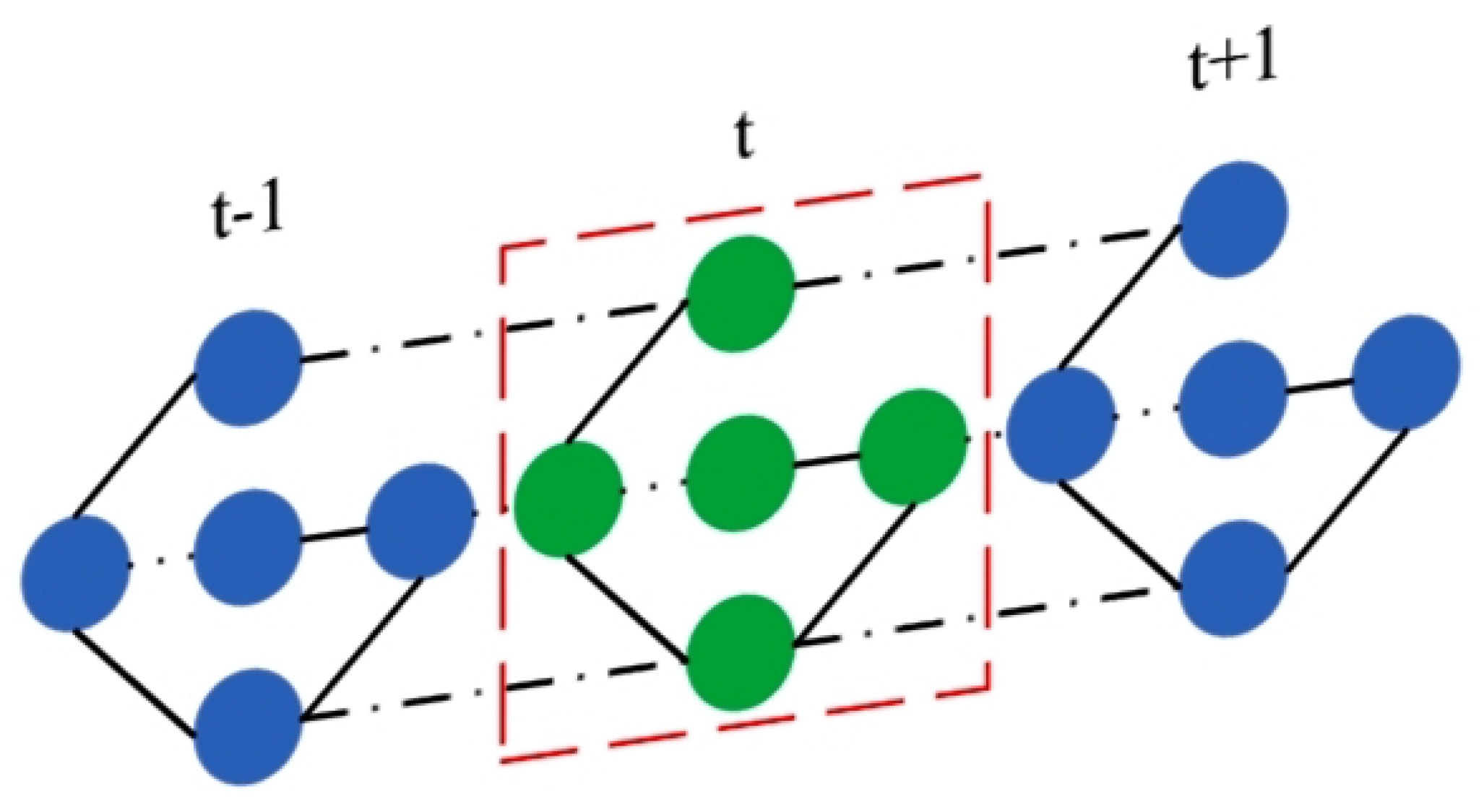
• Cropping operation: The cropping operation consists of removing redundant features from the previous and next time slices from the aggregate results and retaining only features from nodes in the intermediate moments. The reason for this is that the graph convolution operation has already aggregated the information from the previous and next time steps, and cropping two time steps will not result in the loss of important information and each node contains a local spatial-temporal correlation. By stacking multiple GCAMs and retaining the characteristics of all adjacent time-steps, a large amount of redundant information will reside in the model, thereby affecting the prediction effect. The cropping operation is demonstrated in Figure 4, showing cropping of the features of the previous time step $t-1$ and the next time step $t+1$ and keeping the features of the intermediate time step t.

After cropping, the features obtained are input to the CBAM, which can serially generate two sets of attentional feature map information in the two dimensions of channel and space, and then the two sets of feature map information are multiplied with the previous input features for adaptive correction of the features in order to produce the final feature map.

In the first stage, the attention feature map of the channel is generated. This operation can be expressed as follows:

$$h_c=\sigma (W_1\left(W_0\left(AvgPool\left(h_{agg}\right)\right)\right)+W_1(W_0\left(MaxPool\left(h_{agg}\right)\right)\in R^{C\times 1\times 1},$$

(6)

where $W_0\in R^{C/r\times C}$, $W_1\in R^{C/r\times C}$ are learnable parameters, and r is the shrinkage rate. $AvgPool(·)$ denotes average pooling, and $MaxPool(·)$ denotes maximum pooling.

Then, a spatial attention feature map is generated. The input graph is stitched together along the channel with features that are pooled equally and features that are pooled maximally, and convolved by a standard circle base layer to generate a two-dimensional spatial attention graph. This operation can be expressed as follows:

$$h_s=\sigma \left(f^{7\times 7}\left([AvgPool\left(h_{agg}\right);MaxPool\left(h_{agg}\right)]\right)\right)\in R^{N\times T},$$

(7)

where $f^{7\times 7}(·)$ denotes a convolution operation with a convolution kernel size of $7\times 7$.

Finally, the computed spatial feature maps and channel attention maps are used to correct the original input feature maps, and the computation is expressed as follows:

$$Y_{gcam}=h_{agg}\otimes h_c\otimes h_s,$$

(8)

where ⊗ denotes multiplication by bit, when multiplying by bit.

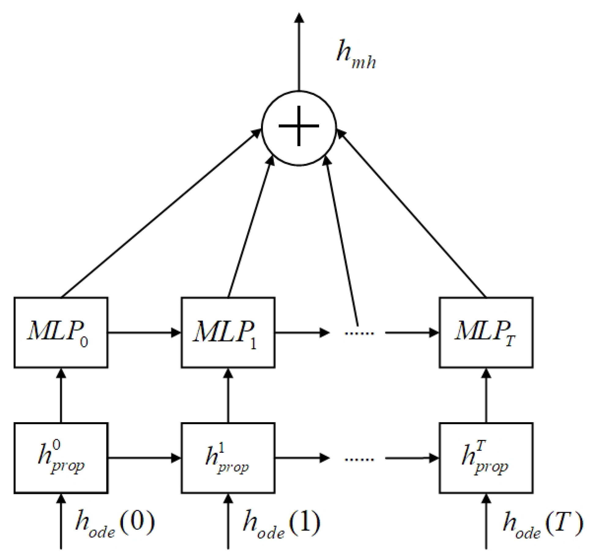
4.3. ODE Spatial-Temporal Graph Convolution Module

We use the ordinary differential equation graph convolution module to extract the long-term spatial-temporal features. Spatial features are first extracted by temporal convolution network (TCN) and spatial features are extracted by graph convolution of ODEs, then by a mix hop layer to prevent the appearance of model over-smoothing [18], and finally by normalization using an activation sigmoid function.

To improve the ability to extract long-term time features, the ODEGCN module uses one-dimensional extended time convolution to extract long-term time features. We first extract temporal features by temporal convolution, and then extract local spatial features by ODESolver. The TCN operation is formulated as follows:

$$h_{tcn}^t=\sigma (\mathrm{\Theta }\ast h_{tcn}^{t-1}),$$

(9)

where $\mathrm{\Theta }$ is the learnable parameter of the convolution filter, and $h_{tcn}^{t-1}$ denotes the input to the TCN of the t time step; when $t=0$, it denotes the initial input.

Based on previous work, we use the method of convolution of ordinary differential equation maps derived from ST-ODE [18] to extract spatial features:

$$h_{ode}\left(t\right)=ODESolve(\frac{dh\left(t\right)}{dt},h_{tcn}^l,t),$$

(10)

After ODESolver processing, we chose to use a mix hop layer [30] to select a portion of the input information to be fused with the processed features in order to prevent over-smoothing. There are two stages in the mix hop layer: propagation of information and selection of information, and the structure is shown in Figure 5. The propagation of information is formulated as:

$$h_{prop}^t=\alpha h_{ode}\left(t\right)+(1-\alpha )\tilde{A}{h}_{prop}^{t-1},$$

(11)

where $\alpha$ is a hyperparameter that controls the ratio of the root node’s initial states retained. $h_{prop}^{t-1}$ denotes the input to the mix hop layer, when $t=0$, $h_{prop}^0=h_{ode}\left(0\right)$. $\tilde{A}={\tilde{D}}^{-1}(A+E)$, ${\tilde{D}}_{\mathrm{ii}}=1+{\sum }_{\mathrm{j}}^{}{\mathrm{A}}_{\mathrm{ij}}$, A denotes an adjacency matrix.

The information selection operation can be expressed as follows:

$$h_{mh}=\sum _{t=0}^T{h}_{prop}^t{W}^t,$$

(12)

where the parameter matrix $W_t$ acts as a feature selector that controls the information flowing from each node to the next node, and $W^t$ is the learnable parameter matrix.

The sigmoid activation function is used to normalize the output of the mix hop layer to give the final output, which is expressed computationally as:

$$Y_{odegcn}=\sigma \left(h_{mh}\right),$$

(13)

4.4. Gated Convolution Model

It is very important to account for the remote temporal correlation of the nodes themselves, and, in order to strengthen the ODEGCN’s ability to extract long spatial-temporal features from the nodes, we parallelize the gated convolution with ODEGCN in order to improve the ability of ODEGCN to extract the long-term spatial and temporal dependence of nodes. In contrast to previous work by GraphWaveNet and STGCN, we introduce the inflation convolution with a large expansion velocity. In view of the total amount of input data $X\in R^{T\times N\times C\times C^{\prime }}$, its form is:

$$Y_{gated}=\varphi ({\mathrm{\Theta }}_1\ast X+a)\odot \sigma ({\mathrm{\Theta }}_2\ast X+b),$$

(14)

where $\varphi (·)$ denotes a tanh function and ⊙ denotes a Hadamar product. ${\mathrm{\Theta }}_1$ and ${\mathrm{\Theta }}_2$ are two independent two-dimensional convolution operations with an expansion rate of 2. It can enlarge the acceptance domain along the time axis and enhance the performance of the model to extract sequence correlation.

4.5. Loss Function

Since Huber loss is less sensitive to outliers and has better robustness, we chose Huber loss as a loss function.

$$L(Y,\widehat{Y})=\left\{\begin{array}{c}\frac{1}{2}{(Y-\widehat{Y})}^2,\left|Y-\widehat{Y}\right|\le \delta \hfill \\ \delta \left|Y-\widehat{Y}\right|-\frac{1}{2}{\delta }^2,otherwise\hfill \end{array}\right.,$$

(15)

where Y denotes the real value, $\widehat{Y}$ denotes the predicted value of the model, and $\delta$ is the threshold parameter that controls the loss range of square error.

5. Experiments

In this study, we validated the performance of LSTFGCN on four datasets of public transport networks, namely PEMS03, PEMS04, PEMS07, and PEMS08, released by Caltrans Performance Measurement System (pms) [31], California. The four datasets, from four different collections of high speed roads, were aggregated into five-minute time steps, i.e., 288 time steps within a day’s traffic flow. For each dataset, the spatial adjacency network was constructed from the true distance-based road network. We used a Z-score to normalize the data inputs. Details are given in

Table 1. Datasets description.

Datasets	Nodes	Edges	Time Steps	Time Range
PEMS03	358	547	26,208	9/1/2018–11/30/2018
PEMS04	307	340	16,992	1/1/201–2/28/2018
PEMS07	883	866	28,224	5/1/2017–8/31/2017
PEMS08	170	295	17,856	7/1/2016–8/31/2016

.

5.1. Experiment Settings

For a fair comparison with previous baseline experiments, we divided all datasets into training sets, verification sets and test sets, with a ratio of 6:2:2, respectively. To predict the next hour of data, we used an hour of historical data, which involves the use of 12 consecutive time steps in the past in order to predict 12 consecutive time steps in the future. We computed LSTFGCN over ten times in each publicly available dataset.

Our implementation of the LSTFGCN model made use of pytorch. Hyperparameters are driven by model performance on the validation dataset. On these four datasets, the best model consists of four LSTFGCNLs, each of which contains three graph convolution operations with 64 filters. The retention rate of the original information in the mix hop layer in ODEGCN is 5%.

5.2. Evaluation Functions

To assess the predictive effect of the model, we used three evaluation indicators that are commonly used in reference articles, including mean absolute error (MAE), root mean square error (RMSE), and mean absolute percentage error (MAPE). The formula is given below:

• Mean Absolute Error (MAE):

  $$MAE=\frac{1}{T}\sum _{i=0}^T\left|Y_i-{\widehat{Y}}_i\right|$$

  (16)

  where $Y_i$ denotes the real value at the i-th time step, and ${\widehat{Y}}_i$ denotes the predicted value of the model at the i-th time step.
• Root Mean Squared Error (RMSE):

  $$RMSE=\sqrt{\frac{1}{T}\sum _{i=0}^T{\left(Y_i-{\widehat{Y}}_i\right)}^2}$$

  (17)
• Mean Absolute Percentage Error (MAPE):

  $$MAPE=\frac{1}{T}\sum _{i=0}^T\left|\frac{Y_i-{\widehat{Y}}_i}{Y_i}\right|$$

  (18)

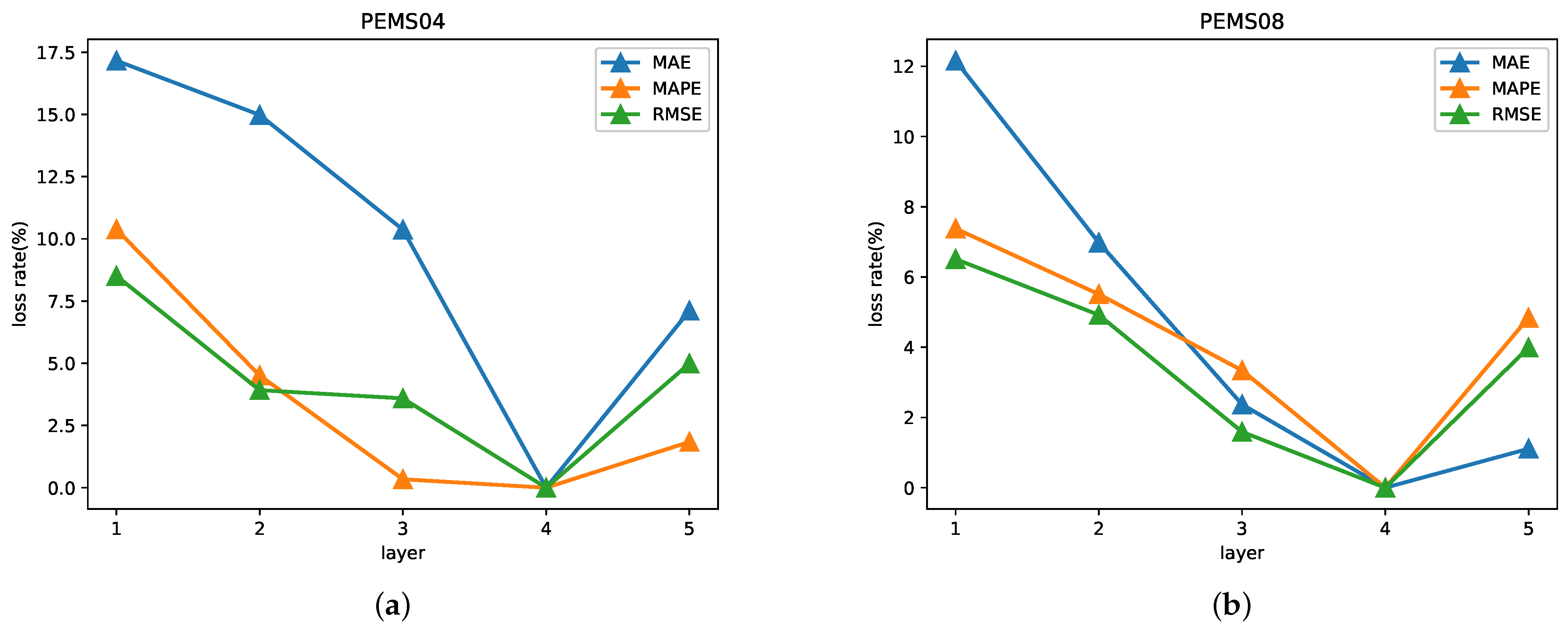
5.3. Study of the Layers of LSTFGCNL

In order to further examine the effect of the number of LSTFGCNL layers on the experimental results, and achieve the best prediction accuracy of the model, we tested 1~5 layers of LSTFGCNL on the PEMS04 and PEMS08 datasets, by selecting the best value of layer depth, and the experimental results are plotted in Figure 6a,b on the two datasets.

As can be seen in Figure 6, all three evaluation metrics on both datasets were optimal when the number of LSTFGCNL layers was four. When the number of LSTFGCNL layers was less than four, the fewer the layers, the worse the model effect, probably because the model failed to fully learn the long short-term spatial-temporal dependencies of nodes due to the small number of layers, which affected the final prediction results. When the number of LSTFGCNL layers was greater than five, the model was overfitted because the deep learning network was too deep, which led to poor final results.

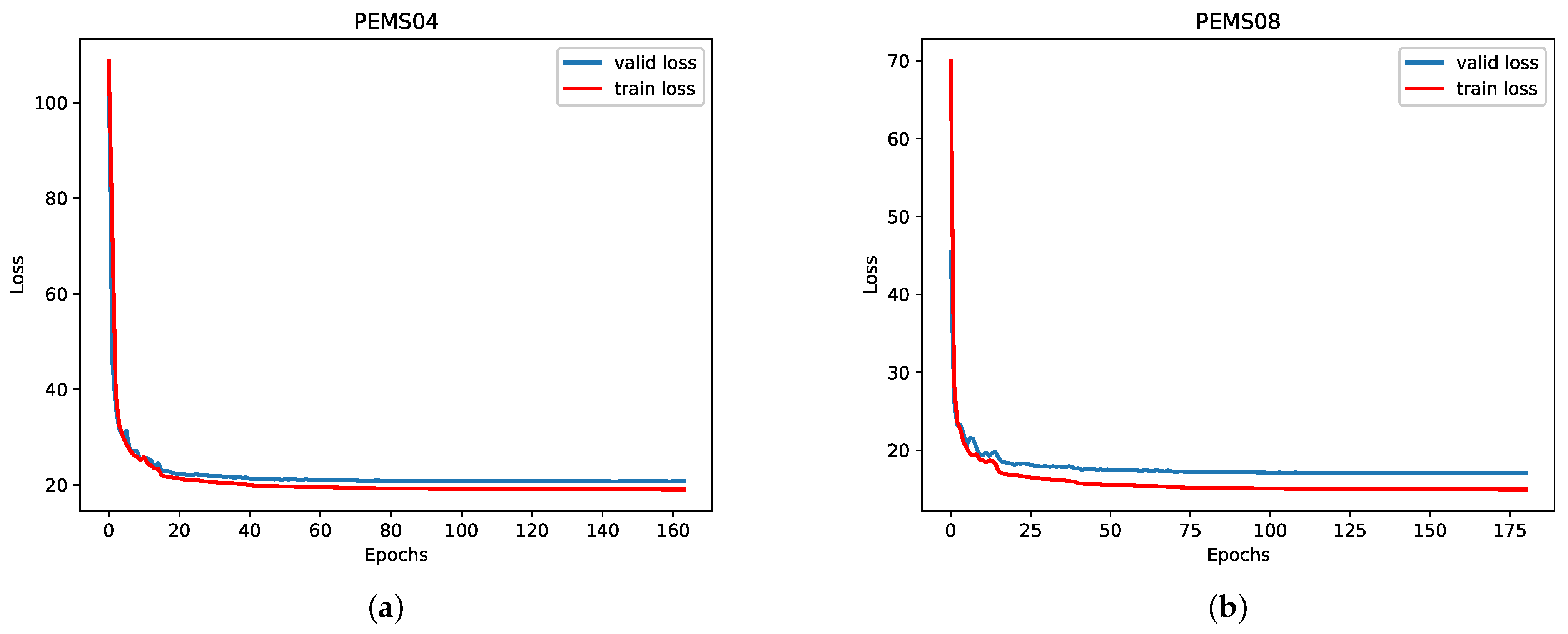
5.4. Convergence Analysis

In order to explore the convergence process of LSTFGCN, we plotted Figure 7a,b representing the training process on the PEMS04 and PEMS08 datasets, respectively. The x-axis in the figure represents the number of training epochs and the y-axis represents the loss value. The figure shows two curves of training loss and validation loss in the training process of the model. It can be seen from the figure that LSTFGCN converged quickly at the beginning and became stable after more than 20 epochs. In the subsequent training, both training loss and validation loss only continued to decrease slightly until the final convergence. In the process of convergence, the two curves were smooth and there were almost no ups and downs, indicating that the model parameters were continuously and stably optimized in the training process.

5.5. Performance Comparison

• FC-LSTM [32]: Long short term memory network (LSTM) is a type of circular neural network that is completely connected to an LSTM hidden unit.
• DCRNN [1]: The cyclic diffusion convolution neural network, which embeds graph convolution into cyclic encoder–decoder units.
• STGCN [2]: Spatial-temporal graph convolution network, integrating graph convolution into one-dimensional convolution units.
• ASTGCN(r) [3]: Attention-based spatial-temporal graph convolution network, which introduces spatial and temporal attentional mechanisms into the model. In order to maintain a fair comparison, only the most recent component of the modeling periodicity is used.
• GraphWaveNet [6]: GraphWaveNet is a framework that combines adaptive adjacency matrices with one-dimensional extended convolution.
• STSGCN [4]: Spatial-temporal synchronous graph convolutional network, which utilizes a local spatial-temporal subgraph module to synchronously capture local spatial-temporal correlativity of node.
• STFGNN [5]: Spatial-temporal fusion graph neural network, which uses the DTW algorithm to construct data-driven graphs to effectively capture hidden spatial dependencies.

The comparison between the various models is shown in

Table 2. Performance comparison of LSTFGCN and baseline models on PEMS03, PEMS04, PEMS07 and PEMS08 datasets.

Datasets	Metric	FC-LSTM	DCRNN	STGCN	ASTGCN(r)	Graph WaveNet	STSGCN	STFGNN	LSTFGCN
PEMS03	MAE	21.33 ± 0.24	18.18 ± 0.15	17.49 ± 0.46	17.69 ± 1.43	19.85 ± 0.03	17.48 ± 0.15	16.77 ± 0.09	16.47 ± 0.05
	MAPE (%)	23.33 ± 4.23	18.91 ± 0.82	17.15 ± 0.45	19.40 ± 2.24	19.31 ± 0.49	16.78 ± 0.20	16.30 ± 0.09	15.51 ± 0.10
	RMSE	35.11 ± 0.50	30.31 ± 0.25	30.12 ± 0.70	29.66 ± 1.68	32.94 ± 0.18	29.21 ± 0.56	28.34 ± 0.46	27.83 ± 0.34
PEMS04	MAE	27.14 ± 0.20	24.70 ± 0.22	22.70 ± 0.64	22.93 ± 1.29	25.45 ± 0.03	21.19 ± 0.10	19.83 ± 0.06	19.71 ± 0.07
	MAPE (%)	18.20 ± 0.40	17.12 ± 0.37	14.59 ± 0.21	16.56 ± 1.36	17.29 ± 0.24	13.90 ± 0.05	13.02 ± 0.05	13.01 ± 0.03
	RMSE	41.59 ± 0.21	38.12 ± 0.26	35.55 ± 0.75	35.22 ± 1.90	39.70 ± 0.04	33.65 ± 0.20	31.88 ± 0.14	31.39 ± 0.20
PEMS07	MAE	29.98 ± 0.42	25.30 ± 0.52	25.38 ± 0.49	28.05 ± 2.34	26.85 ± 0.05	24.26 ± 0.14	22.07 ± 0.11	21.39 ± 0.18
	MAPE (%)	13.20 ± 0.53	11.66 ± 0.33	11.08 ± 0.18	13.92 ± 1.65	12.12 ± 0.41	10.21 ± 1.65	9.21 ± 0.07	9.06 ± 0.09
	RMSE	45.94 ± 0.57	8.58 ± 0.70	38.78 ± 0.58	42.57 ± 3.31	42.78 ± 0.07	39.03 ± 0.27	35.80 ± 0.18	34.86 ± 0.15
PEMS08	MAE	22.20 ± 0.18	17.86 ± 0.03	18.02 ± 0.14	18.61 ± 0.40	19.13 ± 0.08	17.13 ± 0.09	16.64 ± 0.09	16.03 ± 0.02
	MAPE (%)	14.20 ± 0.59	11.45 ± 0.03	11.40 ± 0.10	13.08 ± 1.00	12.68 ± 0.57	10.96 ± 0.07	10.60 ± 0.06	10.15 ± 0.01
	RMSE	34.06 ± 0.32	27.83 ± 0.05	27.83 ± 0.20	28.16 ± 0.48	1.05 ± 0.07	26.80 ± 0.18	26.22 ± 0.15	25.18 ± 0.05

. We can see that our LSTFGCN outperformed the base model on every dataset. Followed by metrics from the previous baseline (STSGCN) takes, Table 2 compares the performance of the LSTFGCN model and the other predicted models 60 min ahead on the PEMS03, PEMS04, PEMS07 and PEMS08 datasets.

LSTM only considers temporal dependence and cannot exploit the spatial dependence of spatial-temporal networks. DCRNN, STGCN, ASTGCN(r) and our LSTFGCN all use spatial information effectively, and have better performance than time series prediction methods. Other methods extract long-term spatial-temporal correlations by sharing a module at different time periods, thus ignoring the heterogeneity of spatial-temporal network data. GraphWaveNet has poor performance because it cannot superimpose its spatial-temporal layers, resulting in a relatively small acceptance domain. Our method constructs a local spatial-temporal subgraph for each node, fully considers the local spatial-temporal correlation using the superimposed spatial-temporal convolution module, and captures more long-term dependencies in the long receptive field of the graph convolution using the combination of ODEGCN and a gated convolution module, whereas STSGCN only extracts local spatial-temporal dependencies, so the experimental results of our method outperformed STSGCN, which is more obvious in datasets with more spatial nodes and time steps.

According to

Table 3. Comparison of prediction results of LSTFGCN and STSGCN on Horizon 3, Horizon 6 and Horizon 12.

Method	PEMS04
	Horizon 3			Horizon 6			Horizon 12
	MAE	MAPE (%)	RMSE	MAE	MAPE (%)	RMSE	MAE	MAPE (%)	RMSE
STSGCN	19.8	13.41	31.58	21.3	14.27	33.83	24.47	16.27	38.46
LSTFGCN	18.77	12.45	29.89	19.64	13.05	31.34	21.37	14.23	33.87
Method	PEMS08
	Horizon 3			Horizon 6			Horizon 12
	MAE	MAPE (%)	RMSE	MAE	MAPE (%)	RMSE	MAE	MAPE (%)	RMSE
STSGCN	16.59	10.98	25.37	17.74	11.56	27.27	20.11	13.04	30.64
LSTFGCN	15.13	9.65	23.58	15.97	10.15	25.14	17.54	11.69	27.61

, compared with STSGCN, our LSTFGCN performed well on both PEMS04 and PEMS08. On the PEMS04 dataset, the MAE and RMSE of LSTFGCN increased by 5.48% and 5.65%, respectively, on Horizon 3, and 8.45% and 7.94%, respectively, on Horizon 6 compared to STSGCN; they increased 14.50% and 13.55%, respectively, on Horizon 12. On the PEMS08 dataset, the MAE and RMSE of LSTFGCN increased by 9.64% and 7.59%, respectively, on Horizon 3 and 11.08% and 8.47%, respectively, on Horizon 6, compared with STSGCN. There was an increase 14.65% and 10.97%, respectively, on Horizon 12. It can be seen from the experimental results that LSTFGCN improved more significantly compared to STSGCN with the longer time step of prediction. Our model has obtained satisfactory results in extracting the long-term spatial-temporal dependence of nodes in both datasets, which proves the competitive advantage of LSTFGCN in long-term prediction.

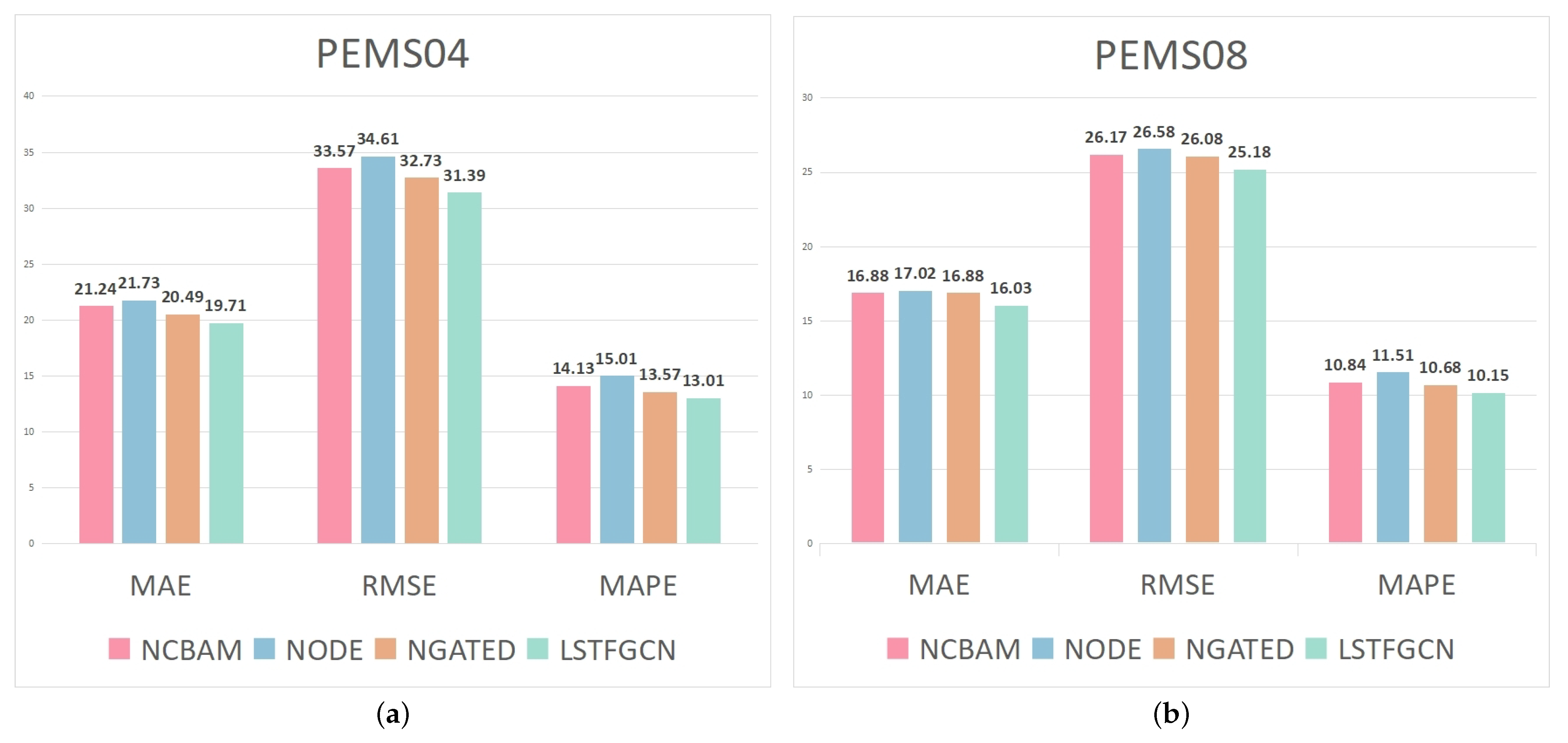
5.6. Ablation Experiments

To verify the effectiveness of different parts of LSTFGCN, we performed ablation experiments on the PEMS04 and PEMS08 datasets. NCBAM, NODE and NGATED denote the CBAM, ODEGCN and gated convolution modules that remove LTSTFGCN, respectively.

Figure 8 shows the measurements of MAE, RMSE and MAPE on three different variant models. After comparison and evaluation with the experimental results of the original model, the following conclusions can be drawn:

• CBAM can carry out adaptive correction to the local spatial-temporal feature map, assign a higher weight to important node information through effective learning, and extract more complex hidden local spatial-temporal dependences.
• The ODEGCN module significantly improves the extraction of long-term spatial-temporal dependence of the model, and obtains more hidden information from longer time series, thus making the model achieve the optimal average prediction results in the end.
• The gated convolution module effectively enhances the ability of ODEGCN to learn the long-term spatial-temporal dependence of nodes, thereby improving the overall performance of the model.

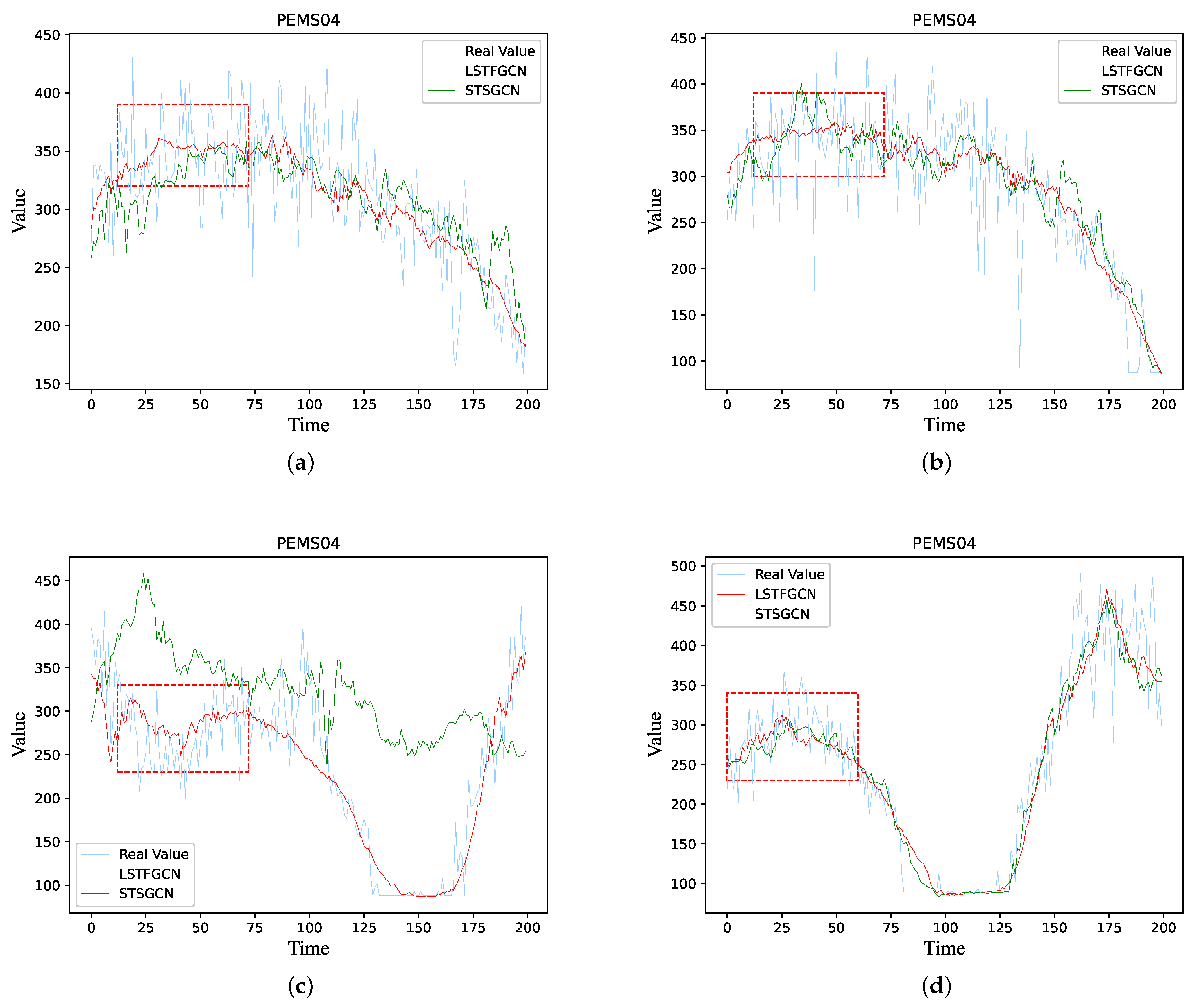
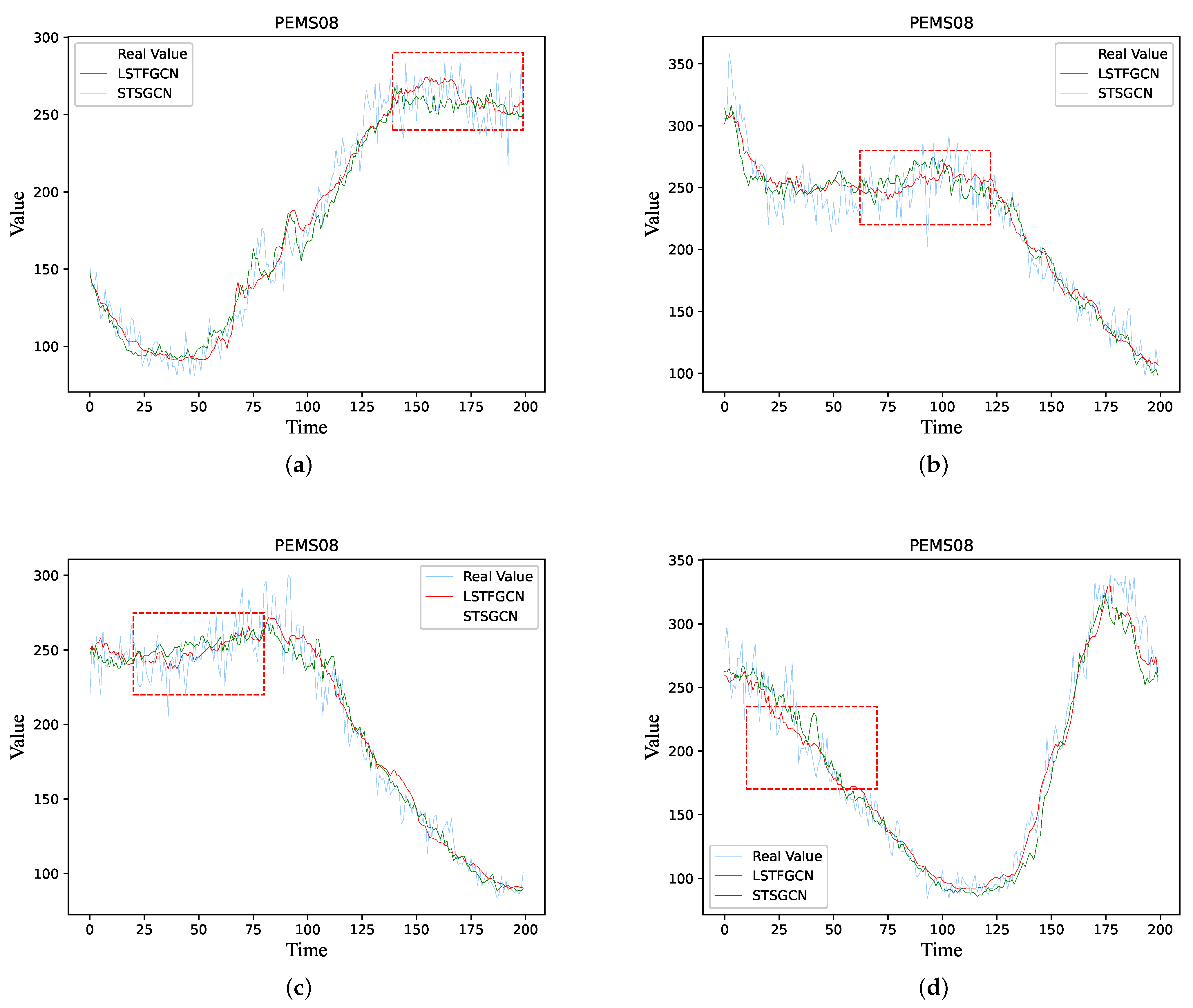
6. Case Study

We compared the Horizon 12 prediction results of STSGCN and LSTFGCN with the actual values of the two datasets, and the end results are demonstrated in Figure 9 and Figure 10. We randomly selected four time step segments from the full time step prediction data of both datasets to compare with the STSGCN prediction results. It can clearly be seen that our model prediction curves fit the true values better and are closer to the true values. In some areas with large fluctuations in traffic flow (e.g., the part framed by the dashed red rectangle), the prediction curves of STSGCN also have large fluctuations and deviate from the true values, while the prediction curves of our model are basically stable at the middle of the fluctuations of the true values, with relatively smooth changes, which match the fluctuation trend of the true values and thus achieve better prediction results.

In Table 2, we compare the average of the three evaluation functions of LSTFGCN with the other baseline models, and demonstrate from the data that the overall prediction of our model is better than the other baseline models. In Table 3, we further perform a comparison of the prediction results of LSTFGCN and STSGCN on Horizon 3, Horizon 6 and Horizon 12, and from the data in the table, we can see that our model outperformed STSGCN in each time step comparison, and the longer the prediction time step, the larger the improvement compared to STSGCN, and the more significant the improvement is, which may be due to the fact that ODEGCN and gated convolution effectively improve the long-term prediction ability of the model. Therefore, it can be concluded that LSTFGCN is closer to the true value compared to STSGCN.

7. Conclusions

In this paper, we propose a new convolutional model of long short-term fusion spatial-temporal graphs for traffic flow forecasting. Our model constructs a local spatial-temporal graph convolution attention module, which effectively synchronously captures the local spatial-temporal dependence of nodes, and the combination of ODEGCN and gated convolution captures more long-term spatial-temporal dependent hidden features of nodes. Then, the fusion module is used to fuse these layers, which can simultaneously learn the long and short-term spatial-temporal dependence features of nodes. Extensive experiments on four real datasets showed that the proposed model outperforms existing models. In addition, an ablation experiment verified the effectiveness of the combination of ODEGCN and gated convolution for the long-term spatial-temporal dependent capture of nodes. However, LSTFGCN designs complex components and superimposes more layers to obtain richer traffic flow features, which incurs additional computational cost and operation time. We plan to redesign a graph convolution construction method for synchronous acquisition of spatial-temporal features, streamline components of different modules to reduce computational overhead, and improve the prediction performance of the model through innovative design integration of the obtained features.

References

1. Li, Y.; Yu, R.; Shahabi, C.; Liu, Y. Diffusion Convolutional Recurrent Neural Network: Data-Driven Traffic Forecasting. In Proceedings of the International Conference on Learning Representations, Vancouver, BC, Canada, 30 April–3 May 2018. [Google Scholar]
2. Yan, S.; Xiong, Y.; Lin, D. Spatial Temporal Graph Convolutional Networks for Skeleton-Based Action Recognition. In Proceedings of the AAAI Conference on Artificial Intelligence, New Orleans, LA, USA, 2–3 February 2018; Volume 32. [Google Scholar]
3. Guo, S.; Lin, Y.; Feng, N.; Song, C.; Wan, H. Attention based spatial-temporal graph convolutional networks for traffic flow forecasting. In Proceedings of the AAAI Conference on Artificial Intelligence, Honolulu, HI, USA, 27 January 2019; Volume 33, pp. 922–929. [Google Scholar]
4. Song, C.; Lin, Y.; Guo, S.; Wan, H. Spatial-temporal synchronous graph convolutional networks: A new framework for spatial-temporal network data forecasting. In Proceedings of the AAAI Conference on Artificial Intelligence, New York, NY, USA, 7–12 February 2020; Volume 34, pp. 914–921. [Google Scholar]
5. Li, M.; Zhu, Z. Spatial-temporal fusion graph neural networks for traffic flow forecasting. In Proceedings of the AAAI Conference on Artificial Intelligence, Virtually, 2–9 February 2021; Volume 35, pp. 4189–4196. [Google Scholar]
6. Wu, Z.; Pan, S.; Long, G.; Jiang, J.; Zhang, C. Graph WaveNet for deep spatial-temporal graph modeling. In Proceedings of the International Joint Conference on Artificial Intelligence, Macao, China, 10–16 August 2019; pp. 1907–1913. [Google Scholar]
7. Woo, S.; Park, J.; Lee, J.Y.; Kweon, I.S. Cbam: Convolutional block attention module. In Proceedings of the European conference on computer vision (ECCV), Munich, Germany, 8–14 September 2018; pp. 3–19. [Google Scholar]
8. Wang, X.; Ma, Y.; Wang, Y.; Jin, W.; Wang, X.; Tang, J.; Jia, C.; Yu, J. Traffic flow prediction via spatial temporal graph neural network. In Proceedings of the Web Conference 2020, Taipei, Taiwan, 20–24 April 2020; pp. 1082–1092. [Google Scholar]
9. Park, C.; Lee, C.; Bahng, H.; Tae, Y.; Jin, S.; Kim, K.; Ko, S.; Choo, J. ST-GRAT: A novel spatio-temporal graph attention networks for accurately forecasting dynamically changing road speed. In Proceedings of the 29th ACM International Conference on Information & Knowledge Management, Virtual, 19–23 October 2020; pp. 1215–1224. [Google Scholar]
10. Chiang, W.L.; Liu, X.; Si, S.; Li, Y.; Bengio, S.; Hsieh, C.J. Cluster-gcn: An efficient algorithm for training deep and large graph convolutional networks. In Proceedings of the 25th ACM SIGKDD International Conference on Knowledge Discovery & Data Mining, Anchorage, AK, USA, 4–8 August 2019; pp. 257–266. [Google Scholar]
11. Bruna, J.; Zaremba, W.; Szlam, A.; Lecun, Y. Spectral Networks and Locally Connected Networks on Graphs. In Proceedings of the 2nd International Conference on Learning Representations, ICLR 2014, Banff, AB, Canada, 14–16 April 2014. Conference Track Proceedings. [Google Scholar]
12. Defferrard, M.; Bresson, X.; Vandergheynst, P. Convolutional neural networks on graphs with fast localized spectral filtering. Adv. Neural Inf. Process. Syst. 2016, 29, 3837–3845. [Google Scholar]
13. Welling, M.; Kipf, T.N. Semi-supervised classification with graph convolutional networks. In Proceedings of the International Conference on Learning Representations (ICLR 2017), Toulon, France, 24–26 April 2017. [Google Scholar]
14. Velickovic, P.; Cucurull, G.; Casanova, A.; Romero, A.; Lio, P.; Bengio, Y. Graph Attention Networks. Stat 2018, 1050, 4. [Google Scholar]
15. Hamilton, W.; Ying, Z.; Leskovec, J. Inductive representation learning on large graphs. Adv. Neural Inf. Process. Syst. 2017, 30, 1024–1034. [Google Scholar]
16. Xu, K.; Ba, J.; Kiros, R.; Cho, K.; Courville, A.; Salakhudinov, R.; Zemel, R.; Bengio, Y. Show, attend and tell: Neural image caption generation with visual attention. In Proceedings of the International Conference on Machine Learning. PMLR, Lille, France, 6–11 July 2015; pp. 2048–2057. [Google Scholar]
17. Liang, Y.; Ke, S.; Zhang, J.; Yi, X.; Zheng, Y. Geoman: Multi-level attention networks for geo-sensory time series prediction. Proc. IJCAI 2018, 2018, 3428–3434. [Google Scholar]
18. Fang, Z.; Long, Q.; Song, G.; Xie, K. Spatial-temporal graph ode networks for traffic flow forecasting. In Proceedings of the 27th ACM SIGKDD Conference on Knowledge Discovery & Data Mining, Singapore, 14–18 August 2021; pp. 364–373. [Google Scholar]
19. Lu, Y.; Zhong, A.; Li, Q.; Dong, B. Beyond finite layer neural networks: Bridging deep architectures and numerical differential equations. In Proceedings of the International Conference on Machine Learning, PMLR, Stockholm, Sweden, 10–15 July 2018; pp. 3276–3285. [Google Scholar]
20. Weinan, E. A proposal on machine learning via dynamical systems. Commun. Math. Stat. 2017, 1, 1–11. [Google Scholar]
21. Chen, R.T.; Rubanova, Y.; Bettencourt, J.; Duvenaud, D.K. Neural ordinary differential equations. Adv. Neural Inf. Process. Syst. 2018, 31, 6572–6583. [Google Scholar]
22. He, K.; Zhang, X.; Ren, S.; Sun, J. Deep residual learning for image recognition. In Proceedings of the IEEE Conference on Computer Vision and Pattern Recognition, Las Vegas, NV, USA, 27–30 June 2016; pp. 770–778. [Google Scholar]
23. Davis, J.Q.; Choromanski, K.; Sindhwani, V.; Varley, J.; Lee, H.; Slotine, J.J.; Likhosterov, V.; Weller, A.; Makadia, A. Time Dependence in Non-Autonomous Neural ODEs. In Proceedings of the ICLR 2020 Workshop on Integration of Deep Neural Models and Differential Equations, online, 26 April–1 May 2020. [Google Scholar]
24. Dupont, E.; Doucet, A.; Teh, Y.W. Augmented neural odes. Adv. Neural Inf. Process. Syst. 2019, 32, 3134–3144. [Google Scholar]
25. Ghosh, A.; Behl, H.; Dupont, E.; Torr, P.; Namboodiri, V. Steer: Simple temporal regularization for neural ode. Adv. Neural Inf. Process. Syst. 2020, 33, 14831–14843. [Google Scholar]
26. Massaroli, S.; Poli, M.; Bin, M.; Park, J.; Yamashita, A.; Asama, H. Stable neural flows. arXiv 2020, arXiv:2003.08063. [Google Scholar]
27. Hanshu, Y.; Jiawei, D.; Vincent, T.; Jiashi, F. On Robustness of Neural Ordinary Differential Equations. In Proceedings of the International Conference on Learning Representations, New Orleans, LA, USA, 6–9 May 2019. [Google Scholar]
28. Glorot, X.; Bordes, A.; Bengio, Y. Deep sparse rectifier neural networks. In Proceedings of the Fourteenth International Conference on Artificial Intelligence and Statistics. JMLR Workshop and Conference Proceedings, Fort Lauderdale, FL, USA, 11–13 April 2011; pp. 315–323. [Google Scholar]
29. Dauphin, Y.N.; Fan, A.; Auli, M.; Grangier, D. Language modeling with gated convolutional networks. In Proceedings of the International Conference on Machine Learning, PMLR, Sydney, Australia, 6–11 August 2017; pp. 933–941. [Google Scholar]
30. Wu, Z.; Pan, S.; Long, G.; Jiang, J.; Chang, X.; Zhang, C. Connecting the dots: Multivariate time series forecasting with graph neural networks. In Proceedings of the 26th ACM SIGKDD International Conference on Knowledge Discovery & Data Mining, Virtual Event, CA, USA, 6–10 July 2020; pp. 753–763. [Google Scholar]
31. Chen, C.; Petty, K.; Skabardonis, A.; Varaiya, P.; Jia, Z. Freeway performance measurement system: Mining loop detector data. Transp. Res. Rec. 2001, 1748, 96–102. [Google Scholar] [CrossRef] [Green Version]
32. Sutskever, I.; Vinyals, O.; Le, Q.V. Sequence to sequence learning with neural networks. Adv. Neural Inf. Process. Syst. 2014, 27, 3104–3112. [Google Scholar]
Figure 1. (a) Urban transport network, where the red points identified as 1 to 5 denote traffic sensors with varying periodicity of sensor time patterns at different locations. (b) Traffic signal tensor map from time t − 1 to t + l + 1, where the traffic flow at the current time step of a node is correlated not only with the previous time step, but also with all historical traffic flows.
Electronics 12 00238 g001
Figure 2. General framework of LSTFGCN.
Electronics 12 00238 g002
Figure 3. Constructed local spatial-temporal graph.
Electronics 12 00238 g003
Figure 4. Cropping operation of h a g g .
Electronics 12 00238 g004
Figure 5. Mix hop layer.
Electronics 12 00238 g005
Figure 6. Loss variation rates for different LSTFGCNL layers on two datasets: (a) experiment loss change rate of different LSTFGCNL layers on PEMS04 dataset; (b) experimental loss change rate corresponding to different LSTFGCNL layers on PEMS08 dataset.
Electronics 12 00238 g006
Figure 7. Training and validation error convergence curves on two datasets: (a) training and validation error convergence curves on the PEMS04 dataset; (b) training and validation error convergence curves on the PEMS08 dataset.
Electronics 12 00238 g007
Figure 8. The experimental results of different variant models: (a) all three evaluation metrics of the variant model on PEMS04; (b) all three evaluation metrics of the variant model on PEMS08.
Electronics 12 00238 g008
Figure 9. Comparison of prediction results of LSTFGCN and STSGCN in four random test cases ahead of Horizon 12 on PEMS04 dataset.
Electronics 12 00238 g009
Figure 10. Comparison of prediction results of LSTFGCN and STSGCN in four random test cases ahead of Horizon 12 on PEMS08 dataset.
Electronics 12 00238 g010