Allocation of Charging Stations for Electric Vehicles Considering Spatial Difference in Urban Land Price and Fixed Budget

Abstract

In this paper, the allocation of charging station (CS) is optimized to alleviate the “range anxiety” of electric vehicle (EV) drivers by reducing the time of medium-to-long distance travel, which is raised due to the potential en-route charging. The problem is defined to explicitly consider the spatial differences in urban land price. Although many works take spatial land price into consideration, few of them notice what the gap of spatial land price bring to the charging system. Our objective function is the expected traveling time under an optimized distribution of urban EV flows, and models of spatial network and CSs allocation are then established. Based on Tabu Search algorithm (TSA), a fixed budget charging resources planning algorithm (FBCRPA) is proposed. The proposed method is compared with methods based on betweeness centrality, and results show that our method can find more effective allocation strategy. It is found that users’ traveling time would decrease with increase in difference in land price. Meanwhile, budget would transfer from central region to other regions and carrying capacity of charging system would improve in the above situation. This paper also finds that increase in budget is beneficial to a reduction in drivers’ time, but the improvement is limited.

1. Introduction

With the serious environmental problems, EV has attracted wide attention from countries as a renewable energy vehicle driven by electricity. The development of EV’s technology and growth of people’s living standard make the quantity of EV increases rapidly. The development and promotion of EV are limited by its own drawbacks, such as limited battery capacity [1]; long charging time. Therefore, the planning of charging infrastructure has a profound impact on the development of EVs. As the main infrastructure for EV to charge, the numbers of CSs and EVs are expected to rise rapidly in the future in line with the National Energy Agency’s goal of 1:1 vehicle-to-pile ratio. EVs have been widely used to carry people or goods because of its popularity. Therefore, the planning of CSs has become an urgent problem. This paper aims at the allocation of CSs and the impact brought by the spatial land price of regions.

In academia, the problem of CS planning has been extensively studied [2,3,4,5,6,7,8,9,10,11,12,13,14,15,16]. In Ref. [2], research has been conducted on CSs’ profit from the operator’s point of view. A heuristic Removing and Merging Possible Locations (RMPL) will screen nodes in the network and ignore the nodes with few profits to obtain: The multi-objective evolutionary algorithm used in Ref. [3] aims to minimize the investment and operation costs of the distribution system while maximizing the annually captured traffic flow. This research mainly focuses on the location of CSs: Reference [4] gives a charging infrastructure planning with the goal to minimize the fleet’s daily charging operation time. Compared with general research, this work focuses on how to manage the fleet. Luo et al. [5] assume that charging services are provided by multiple competitors. Bayesian game is used in this situation so that each of them could get an optimal placement policy. What is more, they found that the CS placement is highly consistent with the heatmap of the traffic flow. Reference [6] focuses on how to balance the charging demand and power network stability. A spatiotemporal model of the charging demand is proposed and a heuristic algorithm involving the grid constraints (HAG) is designed. The utilization of chargers and the carrying capacity of the power network are all improved. Reference [7] presents a Mixed-Integer Non-Linear (MINLP) optimization approach for the optimal placing and sizing of the fast CSs. What is significant is that the robustness and efficacy of the proposed method is studied. Bi et al. [8] study the reasonable layout of CSs by distributing chargers. The nodes, where CSs are located, are selected by the betweenness centrality (BC) in a complex network; In Ref. [9], four methods, i.e., the iterative MILP, greedy approach, effective MILP and chemical reaction optimization, are proposed to minimize construction cost of CSs, and they are evaluated from multiple perspectives. Reference [10] aims to minimize drivers’ charging cost. This work takes EV drivers’ strategic and competitive charging behaviors into account and makes the problem closer to reality. Reference [11] takes the environmental factors and service radius of the CSs into account to minimize total cost of CSs. They set the distance between two CSs with EVs’ reaching distance and choose the location of charging stations with the Voronoi diagram. In Ref. [12], the yearly cost of CSs considering the battery capacity constraint instead of the service radius, which makes the modeling more rigorous and realistic. In Ref. [13], CSs are divided into fast charging and slow charging. At the first stage, we select the best CS locations to minimize EV transportation energy losses. Then, the optimum numbers of slow and fast charging facilities are obtained to minimize the cost and meet demand. In Ref. [14], the LCC criterion is used to assess the project and a modified differential evolution algorithm is adopted to solve the problem. What is creative is that the research object of this work is the battery-swap station rather than the CS. Reference [15] uses regression equations to predict the parking demand variables. They aim to minimize the EV users’ station access costs with considering the parking demand of a vehicle. In Ref. [16], uncertainties existing in the development of future EV technology are properly modeled to ensure the robustness of the planning scheme. It is worth mentioning that this work not only focuses on the present, but also exhibits robustness for all the considered scenarios in the future stage. Reference [17] presents CS Dimensioning and Placement (CSDP) framework for provisioning fast charging infrastructure at minimum cost to accommodate the charging demand of the incremental integration of EVs. The solution can efficiently expand the CS network to accommodate future EV charging and conventional load demands. Reference [18] finds the locations for fast and slow charging stations by analyzing drivers’ daily schedules. A centralised charging station database (CSDB) is employed to reduce the waiting times at charging stations. They find that combining some centralized fast charging stations with many distributed slow charging stations will reduce the charging time. Reference [19] proposes a two-stage CS planning method for sharing EV: In the first stage, the charging stations are sited and sized based on the SEV charging demand estimation. In the second stage, the unsatisfied charging demands are assessed so as to update the charging station capacity accordingly. In Ref. [20], a CS planning model is established to maximize the fuzzy quality of service (FQoS), considering queueing behavior, blocking reliability, and multiple charging options. The results demonstrate that the consideration of FQoS faciliates the finding of the more robust capacity plan. The implementation of the proposed model will be useful for designing a charging station without enough EV arrival and charging service data.

Although above studies have analyzed and optimized the allocation of CSs from various aspects, it should be noted that difference of land price in regions (e.g., spatial land price) is an important factor, which will bring a lot of changes to the problem. References [3,4,6,8,9,12,15,18,20] have not taken spatial land price into considering, this makes them ignore the great impact of spatial land price. Therefore, these works lack some realism. Research such as [3,6,8] notice the construction cost of CS, but they only associate it with the number of chargers. It is obvious that the location would affect the construction cost. References [2,5,7,10,11,13,14,16,17,19] consider spatial land price. In these studies, the construction cost of CS is related to chargers’ number and location. But they just took the construction cost of CS as a parameter; the specific impacts brought by spatial land price and its gap are still left out. The location of CSs and allocation of charging resources are two crucial aspects for EVs’ transportation. Reasonable location and charging resources allocation of CSs can maximize the effectiveness of the limited budget. For example, setting CSs in places with large population and traffic flow may be effective, but it will also bring high construction costs, mainly due to land prices. On the other hand, relatively remote CSs cannot meet the charging demand of EVs and cause unnecessary driving time. Spatial land price will make the value of nodes different and the gap of spatial land price will bring great impacts on the whole system.

In view of the above, construction cost of CSs and importance of nodes are added to the allocation of charging resources. An optimization algorithm is designed for charging resources allocation. The influence brought by spatial land price is studied from multiple aspects and the cause of changes is analyzed and discussed deeply. The major contributions are as follows:

(1)

In order to minimize the traveling time of EVs transporting goods among cities, the model for the allocation of CSs is established with optimized distribution of EV flows. The urban transportation network model is established with spatial network.

(2)

FBCRPA is designed based on TSA to optimize the allocation of EV CSs, which takes land price into account.

(3)

Comprehensive experiments are performed, showing that:

(a)

FBCRPA could give a high-quality budget scheme and it performs better than baseline methods, e.g, nodal-centrality-based heuristic [21].

(b)

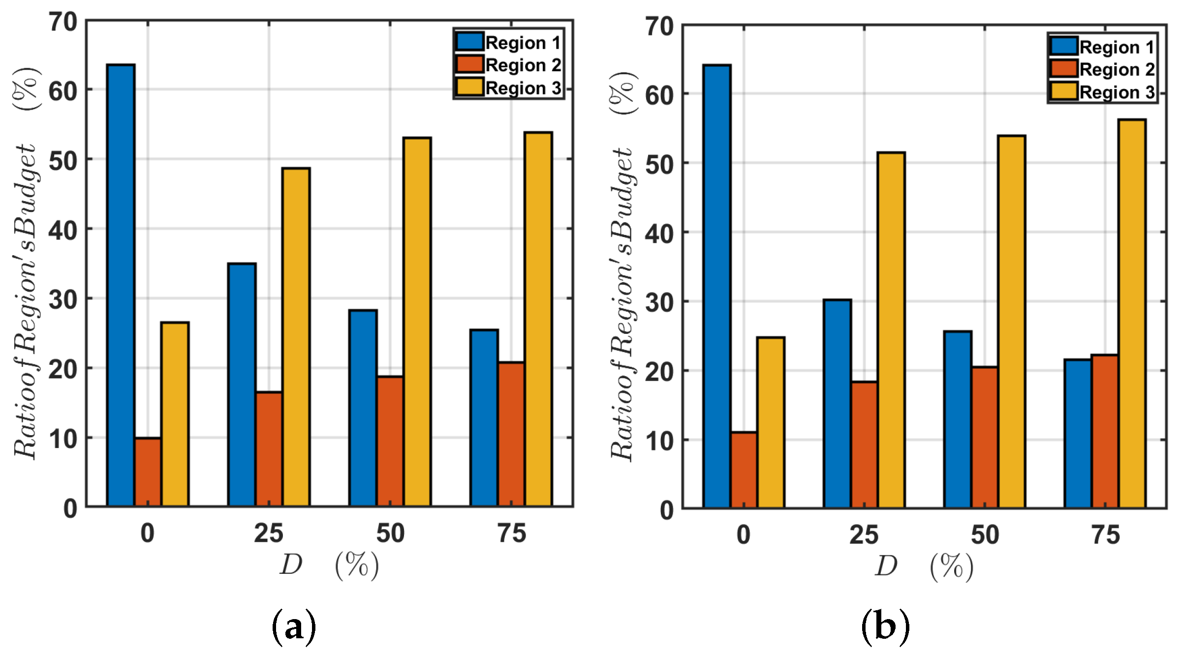
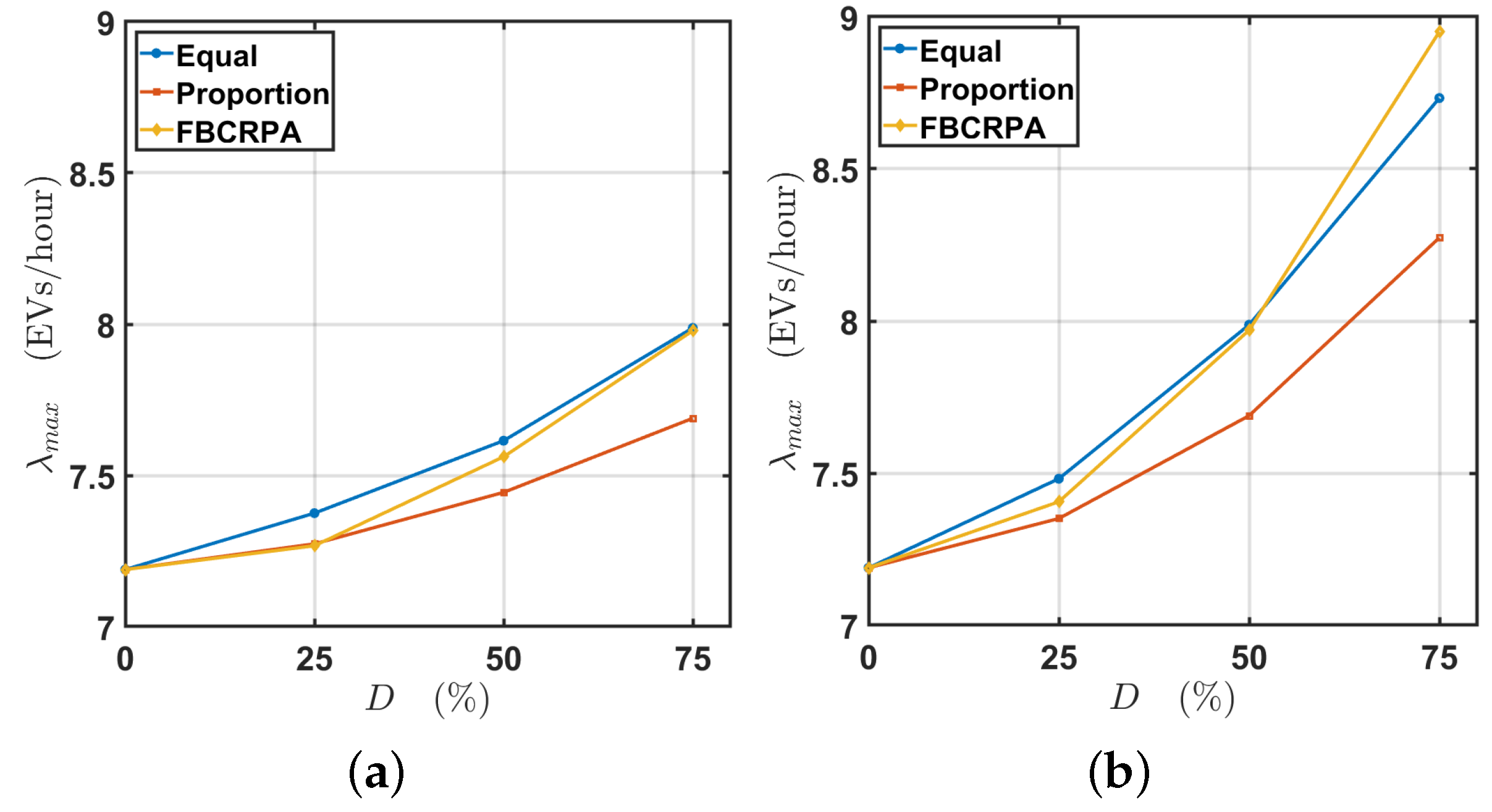
Drivers’ traveling time would decrease with increase in difference in land price. Under the budget scheme given by FBCRPA, the budget would transfer from central region to other regions and the carrying capacity of the charging system would improve.

(c)

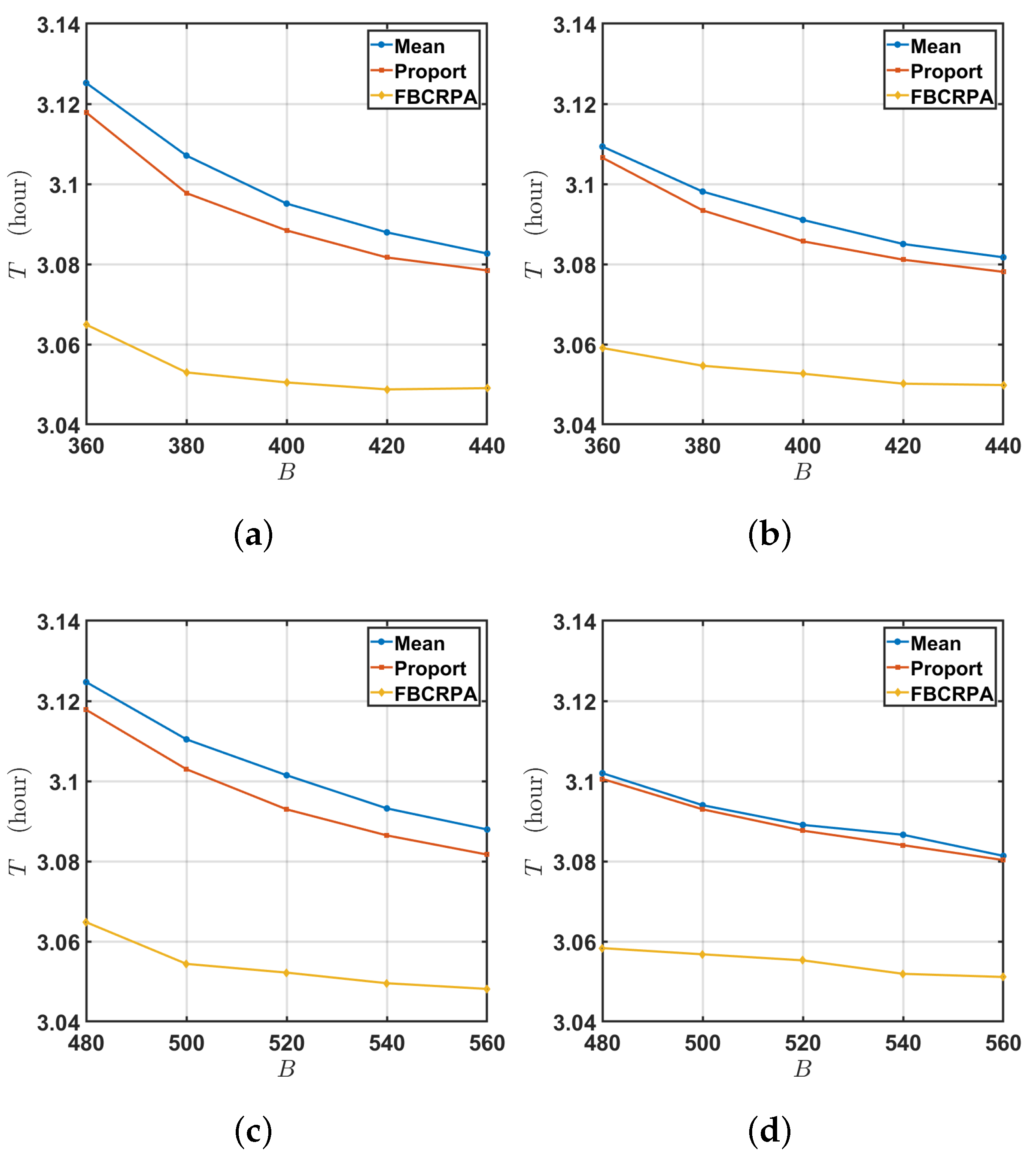
Increasing the budget (for purchasing chargers) can effectively decrease the expected traveling time of passengers, yet there are limits to the benefits of doing so. Moreover, the proposed model facilitate the identification of an “upper bound”, safe-guarding the cost-effectiveness of the investment.

The paper is organized as follows. Section 2 introduces the models and the allocation of CSs, which considers construction cost. Section 3 describes the structure and operation of FBCRPA. In Section 4, the effect of land price difference is researched and discussed. A conclusion is given in Section 5.

2. Models of System and Problem Formulation

The problem of CS planning considering spatial land price and limited budget is studied based on a two-stage optimisation-based model. In the first stage, the allocation of a limited amount of budget is optimised to install additional chargers to CSs, where the land prices are different. In the second stage, the expected distribution of EV flows in the transportation network are optimised to examine the performance of the CS planning solution. The two-stage decisions jointly minimise the expected travel time of individual EV, which consists of on-road driving time and waiting time at charging stations (i.e., queueing and charging). In the following subsections, the modules of the considered two-stage model are respectively introduced.

2.1. Urban Transportation Network Model

In this study, a reasonable urban transportation network model is needed for simulation. The random geometric graph [22] in the spatial network [23] could generate X nodes with random coordinates in the specified space with a side length A, and each node establishes connection with other nodes within connection radius $N_R$. Obviously, nodes located in the center of area usually have higher node importance and connection. Nodes in the urban traffic network usually establish connections with nearby nodes, and important nodes usually located in central area of the city. These characteristics can be reflected in the random geometric graph.

The directed weighted graph $\mathcal{G}$ can be used to represent the above network with charging facilities: $\mathcal{G}=(\mathcal{V},\mathcal{E},\mathcal{A})$. The set of nodes in the urban transportation network is represented by $\mathcal{V}$. The set of nodes located in CSs is ${\mathcal{V}}_c\in \mathcal{V}$. $\mathcal{E}=\left\{\right(i,j\left)\right|i,j\in \mathcal{V},i\ne j\}$, represents the set of edges in the urban transportation network. $\mathcal{A}=\left\{(d_{ij},{\tau }_{ij}^0,q_{ij},{\delta }_{ij})\right|(i,j)\in \mathcal{E}\}$ is the set of weights associated with the edges, where the attributes are defined as follows:

(1)

$d_{ij}$ is the path length of edge $(i,j)$ in urban transportation network, in kilometers;

(2)

${\tau }_{ij}^0$ is the free-flow driving time of the edge $(i,j)$, in hour;

(3)

$q_{ij}$ is the traffic flow capacity of edge $(i,j)$, in EVs/hour;

(4)

${\delta }_{ij}$ is the part of $q_{ij}$ reserved for vehicles without charging demand; it is the realization of a random variable ${\Delta }_{ij}$, which follows a normal distribution, ${\Delta }_{ij}\sim ({\mu }_{ij},{\sigma }_{ij}^2)$.

The following assumptions are made regarding the CSs:

(1)

The CSs allocated at the distribution network of power grids.

(2)

The chargers installed in CSs have same specification and price;

(3)

The queue of EVs at CSs operates on a first-in, first-out principle;

(4)

The charging time of EVs in CSs follows a general distribution, e.g., teuncated normal distribution with mean $\frac{1}{{\mu }_c}$, variance ${\sigma }_c^2$.

2.2. Allocation Model of CSs

The goal of planning will lead to its responding charging resources allocation. In this paper, the problem will be dealt with from the perspective of government. The goal is to minimize the traveling time of the EVs for traveling between locations that requires en-route charging. The problem of CS allocation under land price and limited budget is given by

$$T\left(c\right)=\underset{c^a}{min}\mathbb{E}\left[H^{*}(c,\delta )\right]$$

(1)

$$\mathrm{s}.\mathrm{t}.\sum _{k=1}^{\left|{\mathcal{V}}_c\right|}{c}_k^a{F}_k\le B$$

(2)

$$c=c^a+c^0$$

(3)

$$F_k=C+L_k$$

(4)

where c is the set of chargers in the charging system. $c^0=\left\{c_k^0\in Z^{|{\mathcal{V}}_c|}\right\}$, $c^0$ is the set of chargers initially installed in CS, $c_k^0\ge 0$. $c^a=\left\{c_k^a\in Z^{|{\mathcal{V}}_c|}\right\}$ is the decision vector where $c_k^a$ denotes the number of chargers to be installed at station k, $c_k^a\ge 0$. B represents the total budget in this planning. $H^{*}(c,\delta )$ represents the optimal value of the second stage, which will be detailed in the next section.

Equation (1) represents the charging resources and is allocated to minimize EVs’ traveling time between nodes. Equation (2) means that the budget is limited as B, which is the sum of chargers’ construction cost. The allocation of chargers is composed of initial and additional chargers, which defined by Equation (3). The construction cost $F_k$ of chargers in kth CS is defined by Equation (4), which includes land price $L_k$ and price of charger C.

In order to reflect the spatial land price among regions in the city, the space is divided into R regions according to the distance from the space’s center, $A_r=A/2R$. The diagram of the region is shown in Figure 1.

The land price of each region is different because of its centrality. $C_r$ represents the number of selected nodes in region r to install chargers, $r\in [1,R]$. In the context of network science, the indicators of centrality are widely used to evaluate the importance of nodes. Since the edges of the spatial network are associated with weights, weighted betweenness centrality (BC) is adopted to determine the locations of CSs. $BC$ reflects the dependence of other nodes on one node during information transmission. It is suitable to get the location of charging stations for EVs before going to the destination. The weighted betweenness centrality of a node is calculated by

$$B{C}_k=\sum _{i\ne j\ne k}\frac{{\omega }_{ij}^k}{{\omega }_{ij}},$$

(5)

where ${\omega }_{ij}$ is the number of all shortest (with respect to the length of) paths between $(i,j)$, and ${\omega }_{ij}^k$ is the part of paths passing through node k. In summary, chargers located in different regions will have different performance because of their construction cost and location.

2.3. Model of EV Flow Distribution

In urban transportation network, let $d_r$, $d(m,n)$ be the maximum range of EV and distance from node m to n, respectively. If $d_r<d(m,n)$, then EVs from m to n needs to be charged halfway, and $(m,n)$ is called an unreachable pair. In order to meet charging demand of EVs, the EV flow between the unreachable pair will be allocated to the node set ${\mathcal{V}}_c\subseteq V$ with CSs. Assuming that the EV flow between unreachable pairs follows a Poisson process with an intensity of $\lambda$, a Poisson process will be divided into multiple Poisson processes.

Let $\lambda (m,n)$, ${\lambda }_{ij}^{\left(mn\right)}$ be the EV flow between $(m,n)$ and the flow on $(i,j)$ in $\lambda (m,n)$. The qualified path P would be obtained from tree $T_{mn}$ through ITCA [24]. Based on the above settings, the problem of EV flow distribution could be formulated as

$$\underset{\Lambda }{min}H(c,\delta )=\frac{1}{N}\sum _{\genfrac{}{}{0pt}{}{m,n\in V,m\ne n;}{d_r<d(m,n)}}\left\{\frac{1}{\lambda (m,n)}\sum _{P\subseteq T_{mn}}{\lambda }_P^{\left(mn\right)}{\tau }_P\right\},$$

(6)

$${\tau }_P={\tau }_{L\left(P\right),n}+\sum _{(i,j)\in P}{\tau }_{ij}+\sum _{s_k\in P}\mathbb{E}\left[W^{M/G/c_k}\left(s_k\right)\right],$$

(7)

$${\tau }_{ij}={\tau }_{ij}^0\left[1+\alpha {\left({\delta }_{ij}+\frac{{\lambda }_{ij}}{q_{ij}}\right)}^{\beta }\right],$$

(8)

$$\mathbb{E}\left[W^{M/G/c_k}\left(s_k\right)\right]=\frac{C{V}^2+1}{2}E\left[W^{M/M/c_k}\left(s_k\right)\right],$$

(9)

$$\mathbb{E}\left[W^{M/M/c_k}\left(s_k\right)\right]=\frac{B\left[\lambda \left(s_k\right)\right]}{c_k{\mu }_c-\lambda \left(s_k\right)}+\frac{1}{{\mu }_c}.$$

(10)

Subject to:

$$\sum _{u=C\left(m\right)}{\lambda }_{mu}^{\left(mn\right)}=\lambda (m,n),$$

(11)

$${\lambda }_{ij}^{\left(mn\right)}=\sum _{u=C\left(j\right)}{\lambda }_{ju}^{\left(mn\right)},\forall j\in T_{mn}\setminus \left\{m\cup L\left(T_{mn}\right)\right\},$$

(12)

$${\lambda }_{ij}^{\left(mn\right)}\ge 0,$$

(13)

$${\lambda }_{ij}=\sum _{\genfrac{}{}{0pt}{}{m,n\in V,m\ne n;}{d_r<d(m,n)}}{\lambda }_{ij}^{\left(mn\right)},\forall (i,j)\in \mathcal{E},$$

(14)

$$\lambda \left(s_k\right)=\sum _{(i,j)\in \mathcal{E},j=s_k}{\lambda }_{ij},\forall s_k\in {\mathcal{V}}_c,$$

(15)

$$\frac{\lambda \left(s_k\right)}{c_k{\mu }_c}\le 1-ϵ,\forall s_k\in {\mathcal{V}}_c,$$

(16)

where $\lambda$ is the set of ${\lambda }_{ij}^{\left(mn\right)}$, and ${\lambda }_{ij}$ refers to the EV flow with charging demand on $(i,j)$, in EVs/hour. $\alpha$ and $\beta$ are parameters used to adjust the impact of traffic congestion. $\lambda \left(s_k\right)$ is the EV flow converged at $s_k$, $B\left[\lambda \left(s_k\right)\right]$ is Erlang C formula. N is the number of trees generated in the whole network, that is, the number of unreachable pairs. $CV$ is the coefficient of variation. $C\left(j\right)$ represents the set of children nodes of j. $P\subseteq T_{mn}$ represents a qualified path on tree $T_{mn}$, and the EV flow on it is ${\lambda }_P^{mn}$. $L\left(P\right)$ is the leaf node of path P (excluding the end point n, before n). ${\tau }_P$ represents the sum of driving time and waiting time of EV on path P, which is given by Equation (7). Equation (8) is the Bureau of public roads (BPR) function [25], relating the size of traffic flow to the actual driving time of EVs; Equation (9) obtains the time spent by the EV in CSs through $M/G/K$ model [26] in queuing theory (including queuing and charging), and CS is $s_k$, which equipped with $c_k$ chargers, $K=c_k$; Equation (10) is the average charging time of EV under the exponential distribution charging time of the given parameter ${\mu }_c$. Equations (11)–(16) are constraints on the model. Equations (11)–(12) are the inflow and outflow rate constraint of tree $T_{mn}$; Equation (13) indicates that the flow ${\lambda }_{ij}^{\left(mn\right)}$ cannot be negative; Equation (14) indicates that the total EV flow on $(i,j)$ is the sum of all unreachable pairs passing through $(i,j)$ in the network; Equation (15) uses $\lambda \left(s_k\right)$ to represent EV flow gathered at CS $s_k$; Equation (16) defines the maximum service capacity of $s_k$ for EV; $ϵ$ is the reserved resources to prevent over reception.

3. Design of Algorithm

Local search methods can easily be stuck in suboptimal regions. In comparison, TSA [27] enhances the performance by introducing the so-called Tabu list to discourage the search from going back to solutions that have already been visited. In order to solve the problem of CSs allocation defined by (1)–(4), FBCRPA is designed based on TSA.

3.1. The FBCRPA Building Blocks

(1)

Coding: The candidate solution of additional charging resources allocation is represented by $c^a=\left\{c_k^a\right\}\in {\mathbb{Z}}^{|{\mathcal{V}}_c|}$. $c_k^a$ is the number of chargers to be installed at CS $s_k$.

(2)

Construct Neighborhood: TSA explores the solution space by iteratively moving from one potential solution to an immediate and improved neighbor. The neighborhood structure of FBCRPA is defined as follows:

(a)

Match: Randomly select two CSs $s_1$ and $s_2$ ($s_1,s_2\in {\mathcal{V}}_c,s_1\ne s_2$) to match, and then operate on their respective budgets ($B_{s_1}$ and $B_{s_2}$);

(b)

Shift: For selected budget pair $B_{s_1}$ and $B_{s_2}$, if $B_{s_1}/F_{s_2}$,$B_{s_2}/F_{s_1}\ge 1$ (that is, the budget of one node can at least build a charger at the other node), one of them chosen at random, say $B_{s_1}$, will move $B_{s_1}^r$ to $B_{s_2}$, $B_{s_1}^r\in [F_{s_2},B_{s_1}]$. If one of them, such as $B_{s_2}/F_{s_1}<1$, there is a 50 % chance for $B_{s_1}$ that part of the budget will be given to $B_{s_2}$ according to the above steps. If $B_{s_1}/F_{s_2}$, $B_{s_2}/F_{s_1}<1$, this budget pair will not be operated.

3.2. The FBCRPA Procedures

The FBCRPA’s process is presented in Algorithm 1; $\mathcal{L}$ is a Tabu list, and the maximum number of stored solutions is E; Only $c_s^a$ is stored in the initial $\mathcal{L}$, which is the initial solution randomly generated under Equation (2). It stores the optimal solution of the neighborhood in following steps. In each iteration, a set of neighborhood solution of $c_s^a$ are generated by matching and shifting, namely, $C\left(c_s^a\right)$. If the solution in $C\left(c_s^a\right)$ is not in Tabu list and it can obtain smaller $T\left(c\right)$ than $c_s^a$, $c_s^a$ will be updated. Similarly, if the effect of $c_s^a$ is better than that of $c_{*}^a$, $c_{*}^a$ will be updated. Then free this solution into Tabu list, such a searching cycle loops until the maximum number of iterations is reached.

Algorithm 1 Fixed Budget Charging Resources Planning Algorithm (FBCRPA)

1: Initialize i←0,$c_{*}^a\leftarrow c_s^a$, and $\mathcal{L}\leftarrow c_s^a$ 2: while i≤I do 3:    Do mobile to generate candidate solution set $C\left(c_s^a\right)$ 4:    for all $c^a\in C\left(c_s^a\right)$ do 5:      if $T(c^a+c^0)<T(c_s^a+c^0)$ and $c^a\notin \mathcal{L}$ then 6:            $c_s^a\leftarrow c^a$ 7:         end if 8:      end for 9:      $i\leftarrow i+1$ 10:    if $T(c_s^a+c^0)<T(c_{*}^a+c^0)$ then 11:       $c_{*}^a\leftarrow c_s^a$ 12:    end if 13:    $\mathcal{L}\leftarrow \mathcal{L}\cup \left\{c_s^a\right\}$ 14:    if $\left|\mathcal{L}\right|>E$ then 15:      $\mathcal{L}\leftarrow \mathcal{L}\backslash \left\{{\mathcal{L}}^{\left(1\right)}\right\}$ 16:    end if 17: end while 18:   19: return$c^{*}\leftarrow c_{*}^a+c^0$ and $c_{*}^a$

4. Simulation Result

4.1. Settings for Simulation

In view of EV’s transportation between cities discussed here, a square space with a side length of $A=150$ km is selected as the allocation space of $\mathcal{G}$ (basically equivalent to the scope of a prefecture level city). The space is divided into $R=3$ regions, $A_r=25$ km. In the selected space, it is important to prevent most of selected nodes from being located in central region and ignoring the role of the marginal region. Select $C_1=2$, $C_2=3$ and $C_3=5$ nodes with the largest $BC$ as location of CSs in region 1, 2 and 3, i.e., $|{\mathcal{V}}_c|=10$. The construction costs of chargers in region 1, 2 and 3 are $F_1$, $F_2$ and $F_3$, respectively. For the spatial network model described above, in order to avoid the randomness brought by a single spatial network, the final simulation result is the average of S networks.

In order to locate CSs with a rich candidate solution space, $X=100$ nodes are generated with random coordinates in space. At the same time, set connection radius $N_R$ to 45 km. As transportation of goods is mainly completed by the expressway, this connection radius is just close to the distance between expressway service areas. In view of EV for delivery, e.g., electric vans, E-NV200, its maximum range is 150–200 km, and $d_r$ here is set as 180 km.

Urban land prices are often positively correlated with the importance of region. At the same time, in order to study effect of difference of land price in cities, multiple groups of different land prices can be used for simulation. To simplify the calculation, the price of charger C and average price of all regions are set to 1 and 0.5, respectively, according to the ratio of charger price to land price in reality. Set the total budget of B to 360 and call the case that land price benchmark (M) is 0.5, as shown in

Table 1. $F_k$ of charger in each region with $M=$ 0.5.

Group	${\mathit{F}}_1$	${\mathit{F}}_2$	${\mathit{F}}_3$
1	1.5	1.5	1.5
2	1.625	1.5	1.375
3	1.75	1.5	1.25
4	1.875	1.5	1.125

.

At the same time, the ratio of land price to charger price will also affect $F_k$ of chargers between regions. Therefore, M is set as 1 and C remains 1. To ensure fairness of comparison between two case with M, the B is set as 480. The $F_k$ of the following four groups of chargers is designed as shown in

Table 2. $F_k$ of charger in each region with $M=$ 1.

Group	${\mathit{F}}_1$	${\mathit{F}}_2$	${\mathit{F}}_3$
1	2	2	2
2	2.25	2	1.75
3	2.5	2	1.5
4	2.75	2	1.25

.

In the simulation, the flow distribution process of EV is implemented by the “fmincon” function in MATLAB toolbox [28]. The design of other parameters is shown in

Table 3. Parameters of simulation.

Parameter	Setting
Number of spatial networks $\left(S\right)$	10
Distribution of charging time $\left(\mathcal{N}(\mu ,{\sigma }^2)\right)$	$\mathcal{N}(0.5,0.13)$
truncation interval of charging time distribution	[0.3,0.7]
Utilization of road flow capacity $\left({\Delta }_{ij}\right)$	$\mathcal{N}(0.5,0.1)$
Percentage of reserved charging resources $\left(ϵ\right)$	10%
Number of iterations $\left(I\right)$	100
Length of Tabu list $\left(E\right)$	5
Size of neighborhood $\left(\left|C\left(c_s^a\right)\right|\right)$	5

.

In order to make rational use of charging resources, three budget schemes are used for comparison. Let T, $T_{drive}$, $T_{wait}$ be the average shortest traveling time, the driving time and the waiting time of EV, respectively. The three budget schemes: Equal, Proportion and FBCRPA. Define the total budget as B, then

$$B=\sum _{k=1}^{|{\mathcal{V}}_c|}{B}_k,$$

(17)

where $|{\mathcal{V}}_c|$ is the number of CSs, here it is 10.

The budget scheme of Equal is

$$B_k=\frac{B}{|{\mathcal{V}}_c|}.$$

(18)

The budget allocated to each CS is same. The budget scheme of Proportion is

$$B_k=\frac{B·B{C}_k}{{\sum }_{k=1}^{|{\mathcal{V}}_c|}B{C}_k}.$$

(19)

For comparsion, the percentage of difference in land price is called difference range (D). For example, when M is 0.5, land prices of group 2 are 0.625, 0.5, 0.375, then D of group 2 is $(0.625-0.5)/0.5\times 100\%=25\%$. The D of each group under different M is shown in

Table 4. The D of each group under different M.

Group	Difference Range (D)
1	0%
2	25%
3	50%
4	75%

.

Here, the intensity of EV flow between each unreachable pair in $\mathcal{G}$ is set as $\lambda =6$.

4.2. Performance of Algorithm

In Figure 2, under the same M, the performance of the budget scheme is measured by T. The smaller the T is, the better the performance is. It can be seen from Figure 2 that the budget scheme of FBCRPA performs best, Proportion comes second, and Equal comes third. FBCRPA could obtain a much less T than the other two methods. It can be concluded that the increase in land price difference will lead to the decrease in T in the above spatial network. The specific reasons will be explained in the following steps. At the same time, different M also has an important impact on land price groups with the same D. For example, given the same D, the cases with $M=1$ have smaller T. Under the same D, the actual difference of land price is larger when M = 1. Under the same M, the gap among the three schemes decreases with D increases. That means there is more room for Proportion and Equal to improve, so these two methods decrease faster.

4.3. Impact of Land Price Differences

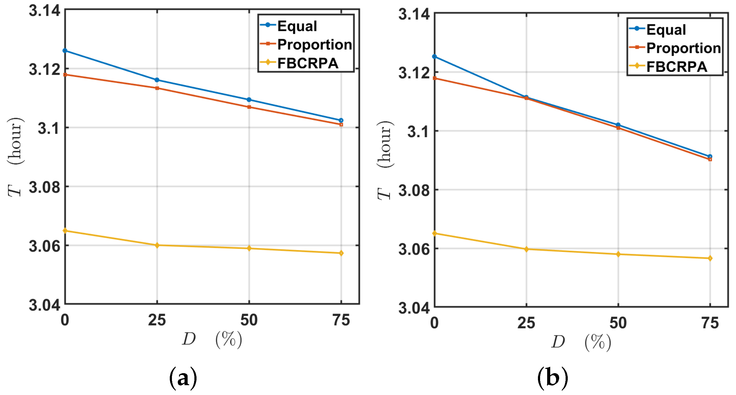
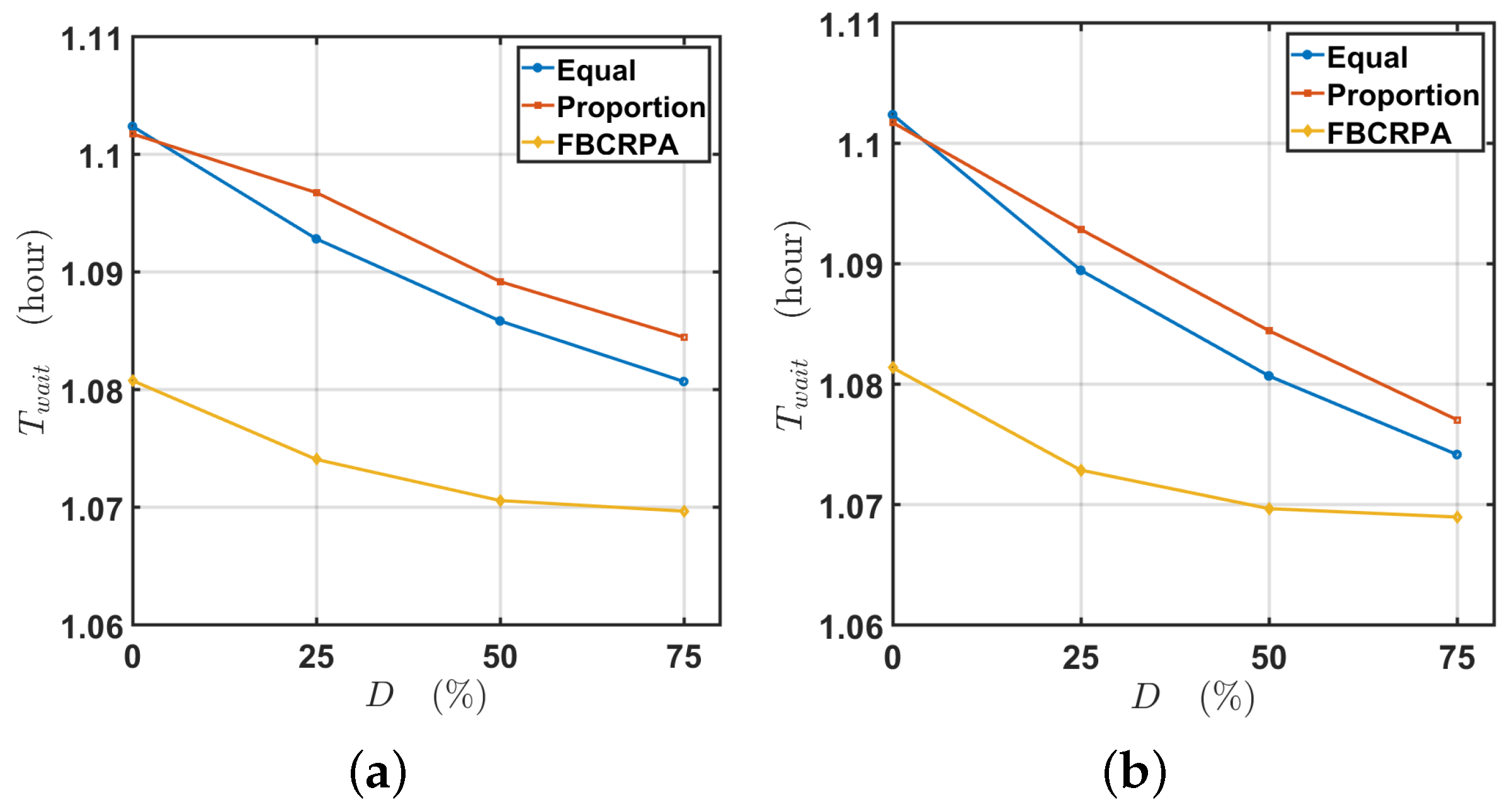
This section will explain the impact of increase in land price difference on T. The parameter setting is same as above.

Figure 3 shows the trend of EV’s waiting time $T_{wait}$ with the increase of land price difference under three budget schemes.

From the analysis of the relationship between $T_{wait}$ and size of D, it can be observed that the trend of T is same as that of $T_{wait}$. This shows that the decrease in T is mainly due to the decrease in $T_{wait}$. For $T_{wait}$, the budget scheme and the number of CSs are two key factors. For example, when land price group is 1 (that is, D is 0), the number of chargers of three budget schemes is same. However, the budget scheme of FBCRPA performs best on $T_{wait}$, Proportion comes second and Equal comes third. This shows that the budget scheme has a key impact on final $T_{wait}$. It can be observed that the allocation of Proportion favors the decrease in $T_{wait}$ more when spatial land price is not considered. FBCRPA is effective in allocating CSs under limited budget. In addition, it can be found that under different M, $T_{wait}$ of Proportion in same land price group is higher than Equal excluding group 1 of the land price. That shows that the decentralized allocation is more beneficial with the spatial land price. However, in the overall performance of T, Proportion’s T is smaller. This means that under Proportion, the budget scheme makes driving time $T_{drive}$ smaller for EVs. In summary, Equal takes more time on driving but its waiting time is smaller with the spatial land price. Proportion is just opposite. The reasons for the decrease in $T_{wait}$ and corresponding impact will be analyzed below.

With a constant budget, the number of chargers that can be built in region 1 decreases, while the number of chargers that can be built in region 3 increases. This is the effect of the spatial land price. Therefore, under FBCRPA’s budget scheme, the budget will be transferred from region 1 to region 2 and 3 for seeking a budget scheme with better performance (the resources allocation of Equal and Proportion is fixed without transfer).

Figure 4 shows the changes in the proportion of regional budgets with the increase in land price difference. It can be observed that in group 1 of the land prices (i.e., when $D=0\%$), the budget proportion of region 1 reaches about 63 %. However, the budget proportion of region 1 is getting lower with the increase in land price difference, while the budget proportion of region 2 and 3 is increasing. Because the land in region 3 is cheaper, the budget of region 2 is obviously lower than that in region 3. The above changes show that with the increase in land price difference, the nodes in region 1 are no longer favored by FBCRPA, and increase in land price difference has brought the transfer of budget. The larger the gap of spatial land price is, the more the budget will transfer to region 2 and 3. As mentioned above, the case $M=1$ actually has a larger difference on land price, which explains why the budget designated to region 1 is smaller when $M=1$. The transfer of budget is the effect of spatial land price difference. At the same time, it also brings some special effects to the charging system.

As mentioned above, the total number of chargers is a key factor. Combined with above analysis, the transfer of budget to regions with low $F_k$ plays a very important role in increasing the number of chargers. This also brings changes in the EV flow carrying capacity of system. According to the constraint formula Equation (16), the carrying capacity of EV flow between unreachable pairs for the spactial network is

$${\lambda }_{max}=\frac{{\sum }_{k=1}^{|{\mathcal{V}}_c|}{c}_k{\mu }_c}{|{\mathcal{V}}_c|}(1-ϵ).$$

(20)

It is easy to see from Figure 5 that with the increase in the land price difference, the carrying capacity of EV flow also increases. This also means that the number of chargers in the whole charging system increases gradually. This is due to the transfer of the budget mentioned above to region 2 and 3. Since more chargers can be built in region 2 and 3 with same budget, the number of chargers in the whole charging system increases.

According to Equation (20), it is clear that the trend of ${\lambda }_{max}$ should be same as that of the total number of chargers in the charging system. The increase in land price difference leads to the increase in the number of chargers, which is one of the key factors leading to $T_{wait}$’s decreasing (in particular, the budget schemes of Equal and Proportion do not change, so the decrease in T is mainly due to the decrease in $T_{wait}$ caused by the increase in the number of chargers). Equal’s chargers are more than Proportion, that could be an important reason for $T_{wait}$ of Equal becoming less than Proportion with spatial land price. Similarly, FBCRPA’s chargers is also larger than Proportion. It can be observed from most land price groups under different M, although ${\lambda }_{max}$ of FBCRPA is smaller than the average distribution most of time (this means fewer charge piles), FBCRPA’s budget scheme has a smaller $T_{wait}$. What is more, the budget allocated by FBCRPA in region 1 is more than Equal in most cases, and the budget allocated in region 2 and 3 is less than Equal, that is why ${\lambda }_{max}$ of FBCRPA is smaller. This shows that except the number of chargers, a reasonable budget scheme is also a key factor. Blindly increasing the number of chargers without selecting a reasonable budget scheme is not cost-effective. As mentioned above, FBCRPA could obtain an effective allocation and relatively large number of chargers.

In summary, the following findings are found in this section:

(1)

It is found that if the total budget remains unchanged, T will gradually decrease as the gap in land price becomes larger. This paper obtains the conclusion that the large difference amplifies the transfer of budgets between regions, leading to more chargers in total. This is also why the decrease in T is primarily driven by the decrease in $T_{wait}$.

(2)

The effectiveness of FBCRPA is proved by comparing with three budget schemes. In cotrast to centrality-based methods, FBCRPA does not blindly increase the number of chargers. Instead, they spend the budget more wisely so that the charging resources can be better utilized by EV flows.

4.4. Impact of Budget

In the research of charging resources allocation in reality, the size of the budget is also a crucial point. Therefore, the relevant research on impact of budget on charging system will be given in Figure 6. Because the trend of T under three budget schemes is similar in each M, group 1 and 3 of land prices are selected from each M. (The comparison between region 1 and region 2 or 4 is similar).

In the above four land price groups, it can be observed that T decreases with the increase in budget. At the same time, the budget scheme of FBCRPA performs best, Proportion comes second, and Equal comes third. In addition, it can be observed that the decline of T slows down with the increase in the budget under three schemes. This shows that the increase in budget does facilitate the decrease in T. However, the impact of increasing the budget on T will be limited gradually. Blindly increasing the budget is also not the most cost-effective choice.

5. Conclusions

A two-stage optimisation-based model considering spatial land price and limited budget is established, which makes results more practical. The model of transportion network is established to reflect spatial land price; the budget is optimised to install additional chargers to CSs. The expected distribution of EV flows in the transportation network are optimised to examine the performance of the CS planning solution. The two-stage decisions aim to minimise the drivers’ traveling time. FBCRPA is designed, which can solve the problem of budget allocation more effectively than centrality-based methods. FBCRPA not only focuses on the number of chargers, but also spends the budget more wisely. It is found that T decreases with the increase in land price difference. Under FBCRPA, the large difference in land prices amplifies the transfer of budgets between regions, leading to the decrease in T and the improvement of carrying capacity. Finally, it is found that the increase in budget is effective but limited to the decrease in T. The efficiency is important for a method or system, the robustness is also critical factor. The robustness of the transportation network refers to the variation of traveling time when there are EVs disobeying the EV flow arrangement. In the future, this work will be conducted to research the impact of spatiality brought to the robustness and how to improve the robustness. Another future direction is to study how vehicle-to-grid (V2G) technology, which enables the power transfer from EV to grid, impacts the CS planning with the presence of spatiality factors such as land price. There have been some studies such as [29,30].

References

1. Bi, X.; Tang, W.K.S. Logistical Planning for Electric Vehicles Under Time-Dependent Stochastic Traffic. IEEE Trans. Intell. Transp. Syst. 2018, 20, 3771–3781. [Google Scholar] [CrossRef]
2. Zhang, Y.; Chen, J.; Cai, L.; Pan, J. EV Charging Network Design with Transportation and Power Grid Constraints. In Proceedings of the IEEE Conference on Computer Communications, Honolulu, HI, USA, 16–19 April 2018; pp. 2492–2500. [Google Scholar]
3. Wang, S.; Dong, Z.Y.; Luo, F.; Meng, K.; Zhang, Y. Stochastic Collaborative Planning of Electric Vehicle Charging Stations and Power Distribution System. IEEE Trans. Ind. Informat. 2018, 14, 321–331. [Google Scholar] [CrossRef]
4. Ma, T.Y.; Xie, S. Optimal fast charging station locations for electric ridesharing with vehicle-charging station assignment. Transp. Res. Part D Transp. Environ. 2021, 90, 102682. [Google Scholar] [CrossRef]
5. Luo, C.; Huang, Y.; Gupta, V. Placement of EV Charging Stations—Balancing Benefits Among Multiple Entities. IEEE Trans. Smart Grid 2017, 8, 759–768. [Google Scholar] [CrossRef] [Green Version]
6. Sun, Z.; Zhou, X.; Du, J.; Liu, X. When Traffic Flow Meets Power Flow: On Charging Station Deployment With Budget Constraints. IEEE Trans. Veh. Technol. 2017, 66, 2915–2926. [Google Scholar] [CrossRef]
7. Sadeghi-Barzani, P.; Rajabi-Ghahnavieh, A.; Kazemi-Karegar, H. Optimal fast charging station placing and sizing. Appl. Energy 2014, 125, 289–299. [Google Scholar] [CrossRef]
8. Bi, X.; Chipperfield, A.J.; Tang, W.K.S. Coordinating Electric Vehicle Flow Distribution and Charger Allocation by Joint Optimization. IEEE Trans. Ind. Informat. 2021, 17, 8112–8121. [Google Scholar] [CrossRef]
9. Lam, A.Y.S.; Leung, Y.W.; Chu, X. Electric Vehicle Charging Station Placement: Formulation, Complexity, and Solutions. IEEE Trans. Smart Grid 2014, 5, 2846–2856. [Google Scholar] [CrossRef] [Green Version]
10. Xiong, Y.; Gan, J.; An, B.; Miao, C.; Bazzan, A.L.C. Optimal Electric Vehicle Fast Charging Station Placement Based on Game Theoretical Framework. IEEE Trans. Intell. Transp. Syst. 2018, 19, 2493–2504. [Google Scholar] [CrossRef]
11. Liu, Z.; Wen, F.; Gerard, L. Optimal Planning of Electric-Vehicle Charging Stations in Distribution Systems. IEEE Trans. Power Del. 2013, 28, 102–110. [Google Scholar] [CrossRef]
12. Li, Y.; Zheng, N.; Zhang, J.; Cai, Q.; Zhong, Z.; Qian, X. Planning Model for Electric Vehicle Charging Station Considering Battery Capacity. In Proceedings of the 2021 IEEE 5th Conference on Energy Internet and Energy System Integration (EI2), Taiyuan, China, 22–24 October 2021; pp. 3768–3771. [Google Scholar]
13. Hayajneh, H.S.; Salim, M.N.B.; Bashetty, S.; Zhang, X. Optimal Planning of Battery-Powered Electric Vehicle Charging Station Networks. In Proceedings of the IEEE Conference on Green Technologies, Lafayette, LA, USA, 3–6 April 2019; pp. 1–4. [Google Scholar]
14. Zheng, Y.; Dong, Z.; Xu, Y.; Meng, K.; Zhao, J.; Qiu, J. Electric Vehicle Battery Charging/Swap Stations in Distribution Systems: Comparison Study and Optimal Planning. IEEE Trans. Power Syst. 2014, 29, 221–229. [Google Scholar] [CrossRef]
15. Chen, T.D.; Kockelman, K.M. The Electric Vehicle Charging Station Location Problem: A Parking-based Assignment Method for Ssettle. 2013. Available online: https://www.caee.utexas.edu/prof/kockelman/public_html/TRB13EVparking.pdf (accessed on 2 February 2022).
16. Wang, G.; Zhang, X.; Wang, H.; Peng, J.C.; Jiang, H.; Liu, Y.; Wu, C.; Xu, Z.; Liu, W. Robust Planning of Electric Vehicle Charging Facilities With an Advanced Evaluation Method. IEEE Trans. Ind. Informat. 2018, 14, 866–876. [Google Scholar] [CrossRef]
17. Kabir, M.; Assi, C.; Alameddine, H.; Antoun, J.; Yan, J. Demand-Aware Provisioning of Electric Vehicles Fast Charging Infrastructure. IEEE Trans. Veh. Technol. 2020, 69, 6952–6963. [Google Scholar] [CrossRef]
18. Schoenberg, S.; Buse, D.S.; Dressler, F. Siting and Sizing Charging Infrastructure for Electric Vehicles with Coordinated Recharging. IEEE Trans. Intell. Veh. 2022. [Google Scholar] [CrossRef]
19. Wang, N.; Wang, C.; Niu, Y.; Yang, M.; Yu, Y. A Two-Stage Charging Facilities Planning Method for Electric Vehicle Sharing Systems. IEEE Trans. Ind. Appl. 2021, 57, 149–157. [Google Scholar] [CrossRef]
20. Zhao, Z.; Xu, M.; Lee, C.K.M. Capacity Planning for an Electric Vehicle Charging Station Considering Fuzzy Quality of Service and Multiple Charging Options. IEEE Trans. Veh. Technol. 2021, 70, 12529–12541. [Google Scholar] [CrossRef]
21. Chen, G.; Wang, X.; Li, X. Fundamentals of Complex Networks: Models, Structures and Dynamics; Wiley: New York, NY, USA, 2015. [Google Scholar]
22. Dall, J.; Christensen, M. Random Geometric Graphs. Phys. Rev. E 2002, 66, 16121. [Google Scholar] [CrossRef] [Green Version]
23. Barthelemy, M. Spatial Networks. Phys. Rep. 2010, 499, 1–101. [Google Scholar] [CrossRef] [Green Version]
24. Bi, X.; Tang, W.K.S.; Han, Z.; Zhou, J. Distributing Electric Vehicles to the Right Charging Queues. In Proceedings of the 2019 IEEE International Symposium on Circuits and Systems (ISCAS), Sapporo, Japan, 26–29 May 2019; pp. 1–5. [Google Scholar]
25. Urban Planning Division: Office of Planning; Bureau of Public Roads: Washington, DC, USA, 1964.
26. Lee, A.; Longton, P. Queueing Processes Associated with Airline Passenger Check-in. J. Oper. Res. Soc. 1959, 10, 56–71. [Google Scholar] [CrossRef]
27. Glover, F.; Laguna, M. Tabu Search. In Handbook of Conbinatorial Optimization; Springer: New York, NY, USA, 1998; pp. 2093–2229. [Google Scholar]
28. MATLAB Optimization Toolbox: Fmincon. In Matlab R2018b; The MathWorks: Natick, MA, USA, 2018.
29. Tirunagari, S.; Gu, M.; Meegahapola, L. Reaping the Benefits of Smart Electric Vehicle Charging and Vehicle-to-Grid Technologies: Regulatory, Policy and Technical Aspects. IEEE Access 2022, 10, 114657–114672. [Google Scholar] [CrossRef]
30. Ye, Z.; Gao, Y.; Yu, N. Learning to Operate an Electric Vehicle Charging Station Considering Vehicle-Grid Integration. IEEE Trans. Smart Grid 2022, 13, 3038–3048. [Google Scholar] [CrossRef]
Figure 1. Diagram of region.
Electronics 12 00190 g001
Figure 2. Performance comparison of three schemes. (a) M = 0.5 , B = 360 . (b) M = 1 , B = 480 .
Electronics 12 00190 g002
Figure 3. T w a i t of three schemes. (a) M = 0.5 . (b) M = 1 .
Electronics 12 00190 g003
Figure 4. Under FBCRPA scheme, the budget proportion of regions under different M. (a) M = 0.5 . (b) M = 1 .
Electronics 12 00190 g004
Figure 5. λ m a x of three schemes. (a) M = 0.5 . (b) M = 1 .
Electronics 12 00190 g005
Figure 6. Relationship between T and budget under different M. (a) D = 0 % , M = 0.5 . (b) D = 50 % , M = 0.5 . (c) D = 0 % , M = 1 . (d) D = 50 % , M = 1 .
Electronics 12 00190 g006