From Beginning to BEGANing: Role of Adversarial Learning in Reshaping Generative Models

Abstract

Deep generative models, such as deep Boltzmann machines, focused on models that provided parametric specification of probability distribution functions. Such models are trained by maximizing intractable likelihood functions, and therefore require numerous approximations to the likelihood gradient. This underlying difficulty led to the development of generative machines such as generative stochastic networks, which do not represent the likelihood functions explicitly, like the earlier models, but are trained with exact backpropagation rather than the numerous approximations. These models use piecewise linear units that are having well behaved gradients. Generative machines were further extended with the introduction of an associative adversarial network leading to the generative adversarial nets (GANs) model by Goodfellow in 2014. The estimations in GANs process two multilayer perceptrons, called the generative model and the discriminative model. These are learned jointly by alternating the training of the two models, using game theory principles. However, GAN has many difficulties, including: the difficulty of training the models; criticality in the selection of hyper-parameters; difficulty in the control of generated samples; balancing the convergence of the discriminator and generator; and the problem of modal collapse. Since its inception, efforts have been made to tackle these issues one at a time or in multiples at several stages by many researchers. However, most of these have been handled efficiently in the boundary equilibrium generative adversarial networks (BEGAN) model introduced by Berthelot et al. in 2017. In this work we presented the advent of adversarial networks, starting with the history behind the models and c developments done on GANs until the BEGAN model was introduced. Since some time has elapsed since the proposal of BEGAN, we provided an up-to-date study, as well as future directions for various aspects of adversarial learning.

1. Introduction

In an effort to mimic the functionality of a human brain more closely than previously achieved by neural networks, researchers have attempted to train deeper networks. Their architectures have proved capable of representing some complex functions which could not be represented as efficiently otherwise [1]. A function can be expressed by using a composition of computational elements from a given set. It has been observed that a function which has compact representations using architecture of depth k may require an exponential number of computational elements if an architecture of depth k-1 is used, thereby establishing a benefit of depth [2]. These layers are not designed by human engineers but are learned from data using a general-purpose learning procedure. Classification-based machine learning algorithms are often classified into two categories based on the estimation criterion they use for adjusting their parameters and/or structure, namely discriminative and generative models.

Discriminative models focus only on the conditional relation of the label given in the training data; the classification objective is used to optimize their parameterized decision boundaries leading to a large margin of separation for the classes; however, they traditionally require that all classes be considered simultaneously. Discriminative models generally produce robust and highly accurate classes and are used for specified tasks such as classification or prediction, with support vector machines and boosting algorithms.

Generative models, on the other hand, work with a joint probability distribution over the examples and the labels i.e., they can be trained with missing data and can predict the output on inputs corresponding to the missing data. These models enable machine learning to work with multi-modal outputs [3]. Time-series data may be used in generative models to simulate possible futures. Some tasks, such as single image super resolution, the creation of art, and image-to-image translation, require realistic generation of samples from some distributions: this can be achieved with generative models. Thus, generative models have the ability to create new input datasets based on outputs that do not belong in the original training dataset, marking the next stage of machine intelligence after classification and regression: synthetization and generation. This ability opens up new avenues for machine learning and allows for more noteworthy contributions to a wider range of applications and implementations. For example, generative models can be used for generating images of faces and places that do not exist [4].

Generative models have been a popular research subject for the past half-decade, with numerous new architectures being introduced at breakneck speed. This rapid development has created a branch of machine learning that can be called a field of its own. One of the major breakthroughs in the efficiency and efficacy of successful generative models is the development of the adversarial model of generative Networks. As GANs only need an arbitrary latent vector to generate realistic samples, they are powerful and have been applied widely in a variety of fields. GANs are well known for their applications involving digital images, such as generation, in-painting, person re-identification, super-resolution, and object detection. They have also been used in video generation, image-to-image translation, text-to-image translation, and the generation of deep-fakes. They have also been used to generate human speech and music [5]. With major developments in research, GANs are becoming more sophisticated and powerful, and are spreading to use in various fields including academia, entertainment, and healthcare.

Two terms which play a significant role when a robust machine learning model is built are generalization and regularization. The ability to process the new data of a system is called generalization. This process helps the system in generating accurate predictions. The generalizing capability of a system is reflected in its success. Generalization is likely to be prevented in the case when the system is over-trained. It may produce inaccurate results when new data is fed to the system. In such cases, when new data is supplied, it will make inaccurate predictions. This situation is termed as overfitting. Overfitting occurs when a network performs well on the training set but performs poorly in general. In a sense, generalization deals with the model’s behavior. On the other hand, it is responsible for enhancing the model performance. Similarly, it is said that under-fitting occurs when a model is trained with insufficient data. It has its effects on the system to such an extent that, even given the training data, the model may not produce correct results. As a result, the system becomes ineffective like the case of overfitting. This also leads to poor generalization. Regularization prevents overfitting by discouraging the learning of a more complicated or flexible model. In a straightforward way, regularization has no effect on the algorithm’s performance on the datasets used to learn the feature weights of the model. However, it enhances the performance of generalization. It means that the algorithm performs better on newly taken and previously unknown data. In a nutshell, it can be said that regularization helps the machine learning models to improve generalization.

The development of various gradient descent methods, and the improvement of network structures and their connectivity style have smoothened the optimization of deep learning. So, the effectiveness of a network depends upon its generalization ability. This has been an efficient way to improve the generalization ability of deep CNN, because it makes it possible to train more complex models while maintaining a lower overfitting. In [6] an approach is presented to optimize the feature boundary of deep CNN through a two-stage training method (pre-training process and implicit regularization training process) to reduce the overfitting problem. This approach has been verified to be effective and provides better results, and also, through a variety of strategies to explore and analyze the implicit role of regularization in the two-stage training process. The Voxel Embed: 3D instance segmentation and tracking with Voxel embedding-based deep learning [7,8,9,10,11]. An application of this process applied to face recognition was obtained in [12] and for action recognition in [13].

Generative adversarial networks (GANs), which are the main focus of this paper, are a class of generative models that work by training a generative model in competition with a discriminative model [14]. To understand the necessity that fueled the development of adversarial networks, it is first necessary to conduct a preliminary study of the taxonomy of non-adversarial generative networks with a focus on the maximum likelihood estimators discussed in Section 2. In Section 2, we also introduce adversarial networks. From Section 3, Section 4, Section 5, Section 6, Section 7, Section 8, Section 9, Section 10, Section 11 and Section 12, we discuss specific relevant image- or video-based generative adversarial models [15] including: generative adversarial networks [16,17], conditional adversarial networks, deep multi-scaled video prediction beyond MSE, adversarial autoencoders, deep convolutional GANs, energy-based GANs, least square GANs, adaptive GANs (AdaGANs) [18], Wasserstein GANs, and BEGANs [19]. In Section 13, Section 14, Section 15 and Section 16, we discuss specific developments on, or use-cases of, image-based GANs in the order of creative adversarial networks (CANs), improved learning techniques, visual manipulations, and image-to-image translation. In Section 17, we discuss how GANs can be used outside image-related domains via speech enhancement GANs. Section 18 discusses recent developments in research with regard to GANs, and Section 19 discusses possible future avenues for research. Finally, the paper is concluded in Section 20.

2. Non-Adversarial Generative Networks

Generative models usually work by estimating a function that allows it to generate input data matching an output that was not present in the training data. Two major estimators used in generative models are density estimation models and maximum likelihood estimators (MLEs). Density estimation models take a training set of examples drawn from an unknown data-generation distribution PD and return an estimate probability distribution PM of that distribution, such that PM can be evaluated at every value $x$ to obtain an estimation PM($x$) of the true density of $x$ [20]. In some cases, PM is explicitly estimated, while in other cases only samples of PM are generated by the model. Some models are able to do both.

In this paper, we restricted ourselves to deep generative models that work by maximizing likelihood, as GANs fall in this category. In statistics, maximum likelihood estimation [21] is a method for estimating the parameters of a statistical model given some observations, by finding parameter values that maximize the likelihood of the making of observations if the parameters were given. The basic idea behind MLE is to define a model that provides an estimate of a probability distribution, using a parameter $\theta$. Then, the likelihood is the probability that the model assigns to the training data ${\pi }_{i=1}^{m}PM(x^{(i)},\theta )$ for a dataset containing m training examples $x^{(i)}$.

Speaking literally, the principle of maximum likelihood requires selecting those parameters for the model that maximize the likelihood of the training data occurring. In Equation (1), the logarithm function is used as it increases everywhere and does not change the location of the maximum. MLE can be explained in the following computations.

If ${\theta }^{*}$ is the optimum value of the likelihood function then,

$$\begin{array}{ll}{\theta }^{*}& =\underset{\theta }{\arg \max }{\pi }_{i=1}^{m}PM(x^{(i)},\theta )\\ & =\underset{\theta }{\arg \max }\log {\pi }_{i=1}^{m}PM(x^{(i)},\theta )\\ & =\underset{\theta }{\arg \max }{\displaystyle {\sum }_{i=1}^m\log }PM(x^{(i)},\theta )\end{array}$$

(1)

MLE can be seen as a special case of the maximum posteriori estimation (MAP) that assumes a uniform prior distribution of the parameter $\theta$. MAP is an estimate of an unknown quantity that equals to the mode of the posterior distribution. MLE can also be seen as a variant of the MAP that ignores the prior and therefore is not regularized.

If we consider MLE-based generative models to be a class on their own, then the taxonomy of this classification can be given by Figure 1. This consists of two major categories, namely explicit and implicit density-based models, where GANs are classified in the latter category.

2.1. Explicit Density Models

These models provide explicit density functions which are intractable and require the approximation to optimize the likelihood. There are two categories under this group; the models under the first category use deterministic approximations, mostly leading to variational methods and the other category use stochastic approximations, which are mostly Markov chain Monte Carlo methods.

For these models, an explicit density function $PM(x,\theta )$ is defined, that is, there is a prior distribution assumed on the data [22]. The model’s definition of density function is put into the expression for the likelihood, and this is maximized using the gradient uphill method. One drawback of explicit density models is in designing a model that captures all the complexity of data to be generated and is still computationally tractable. To handle this problem, models are constructed such that their structures guarantee tractability and others are constructed to admit tractable approximations to the likelihood and its gradients. The tractability of an explicit density function is the ability to define a parametric function that is able to capture the distribution effectively. Explicit density models can be divided based on whether they are tractable or not, into structures of tractable density and structures of approximate density, respectively.

2.1.1. Structures of Tractable Density

Structures of tractable density, as their name suggests, have a density that can be solved or is assumed to be solvable. That is, for such models, the density is assumed to be definite and known. Five major models fall under this category: fully visible belief networks (FVBNs); change of variables models such as nonlinear independent components analysis (nonlinear ICA); neural autoregressive distributed estimator (NADE); masked autoregressive for distribution automation (MADE); and PixelRNN.

Fully visible belief networks (FVBNs): FVBNs fall among the three most popular approaches to generative modeling, along with generative adversarial networks (GANs) and variational autoencoders. This model uses the chain rule of probability to decompose a probability distribution of an n-dimensional vector into a product of one-dimensional probability distributions:

Let $x=(x_1,x_2,\dots ,x_n)$, then the formula is given by Equation (2).

$$PM(x)={\pi }_{i=1}^{n}PM(x_i|x_1,x_2,\dots x_{i-1})$$

(2)

FVBNs are both computationally expensive, as the distribution over each x is computed by a deep neural network, and resistant to parallelization. Due to this, generation via FVBNs is time consuming and unsuitable for real-time applications. GANs, on the other hand, are capable of generating all of x in parallel, greatly reducing computation time.

Nonlinear independent components analysis (Nonlinear ICA): Nonlinear ICAs are another popular tractable density method and are often mentioned in comparison to FVBNs and GANs. They are based on the definition of a continuous, non-linear transformation of data between two different spaces or dimensionalities. As the name suggests, it attempts to represent the observed data as statistically independent component variables.

In Equation (3), a vector of latent variables $z$ and $a$ continuous, differentiable, invertible transformation $g$ is considered such that $g(z)$ yields a sample from the model in $x$ space.

$$px(x)=pz(g^{-1}(x))|\det ((\partial g^{-1}(x))/\partial x)|$$

(3)

One member of this family is the real-valued non-volume preserving (real NVP) transformations, a set of powerful, stably invertible, and learnable transformations, resulting in an unsupervised learning algorithm with exact log-likelihood computation, exact and efficient sampling, exact and efficient inference of latent variables, and an interpretable latent space.

The transformation $g$ can be designed such that the density is tractable; however, the model requires that the transformation be continuous, differentiable, and invertible. The invertibility constraint requires that x and z must have the same dimensions. This means that to generate 5000 pixels, you need to have 5000 latent variables within the model to allow it to work efficiently [23]. On the contrary, GANs put no such restriction on g and do not impose any restrictions on z and x as stated above.

Neural Autoregressive Distributed Estimator (NADE): Neural autoregressive distributed estimator (NADE) models are neural network architectures that can be applied to the problem of unsupervised distribution and density estimation. They leverage the probability product rule and a weight sharing scheme inspired from restricted Boltzmann machines, to yield an estimator that is both tractable and has good generalization performance [24].

Masked Autoregressive Distributed Estimator (MADE): Masked autoregressive models use a binary mask matrix for an element wise multiplication for each matrix to zero connections so as to fulfill the autoregressive property. Here, computing the negative log-likelihood is equivalent to sequentially predicting each dimension of input x [25].

PixelRNN: PixelRNN is a deep neural network that sequentially predicts the pixels in an image along with the two spatial dimensions. This method models the discrete probability of the raw pixel values and encodes the complete set of dependencies in the image. Architectural novelties include fast two-dimensional recurrent layers and an effective use of residual connections in deep recurrent networks [25].

2.1.2. Variational Approximations

Variational methods define a lower bound as in Equation (4).

$$L(x;\theta )\le \log PM(x;\theta )$$

(4)

Any learning algorithm that maximizes L must obtain as high a value as log likelihood. Variational autoencoder is one among the top three popular models, along with FVBN and GAN. In practice, variational methods often obtain very good likelihood, but the generated samples are regarded as lower quality samples. However, measuring sample quality is a subjective opinion as there is no quantitative measure for it. Although GANs are supposed to generate better sample quality, it is difficult to specify any single aspect which is responsible for a better or worse sample quality. The main drawback of the variational methods is that when too weak of an approximate posterior distribution or too weak of a prior distribution is used, even with a perfect optimization algorithm and infinite training data, the gap between L and the true likelihood can result in PM learning something other than the true PD.

Variational Auto Encoder (VAE): VAEs are appealing because they are built upon standard function approximators (neural networks) and can be trained with stochastic gradient descent. VAEs have already shown promise in generating many kinds of complicated data, including handwritten digits, faces, house numbers, CIFAR images, physical models of scenes, segmentation, and predicting the future from static images [26].

2.1.3. Markov Chain Approximations

Usually, sampling-based approximations work reasonably well as long as a fair sample can be generated quickly and the variance across samples is not too high. In some cases, Markov chain techniques are used to generate more expensive samples.

A Markov chain is a process for generating samples by repeatedly drawing a sample $x\prime ~q(x\prime /x)$. Here q is a transition operator. Markov chain methods can sometimes guarantee that x will eventually converge to a sample from PM(x). However, this process cannot always be predicted to converge and even if it converges the process is very slow. In high dimensional spaces, Markov chains become less efficient. Boltzmann machines are an example of such models, and their present-day use is limited due to this drawback. While Markov chain approximations may be efficient in the training process itself, the process of generating samples from the trained model is computationally considerably more expensive than single-step generation methods.

Restricted Boltzmann Machines: A restricted Boltzmann machine (RBM) [27] is a generative stochastic artificial neural network that can learn a probability distribution over its set of inputs. As the taxonomy indicates, RBMs are a variant of Boltzmann machines, with the restriction that the neurons must form a bipartite graph: a pair of nodes from each of the two groups of units (commonly referred to as the “visible” and “hidden” units respectively) may have a symmetric connection between them; and there are no connections between nodes within a group.

2.2. Implicit Density Models

In implicit density models, the training is carried out without specifying the density functions explicitly. The training is provided to the model while interacting indirectly with PM and mostly just sampling from it.

Some models under this category draw samples from PM and define a Markov chain transition operator which is run several times in order to get a sample from the model. An example of this type of network is the generative stochastic model. However, as any model using Markov chains, they face difficulty in scaling high dimensional spaces and have significantly high computational costs. GANs are an exception to this, despite utilizing Markov chains, they avoid these issues by generating the samples in a single step.

Some implicit density models function on kernelized moment matching, such as the generative moment matching networks. Here, deep neural network kernels are used to learn a deterministic mapping from a simple and easy to sample distribution, to samples from the given data distribution by minimizing the maximum mean discrepancy. The training can be scaled to large datasets using minibatch stochastic gradient descent.

2.2.1. Goal-Seeking Neural Networks (GSN)

The GSN model has been generated in response to a number of observed weaknesses in the probabilistic logic node (PLN) proposed by Kan [28]. Filho et al. [29] identify these problems and show how the goal-seeking nature of the GSN overcomes them. The GSN is designed to make efficient use of its memory space by reducing its internal representation and allowing new patterns to be learned without overwriting existing memories. This is achieved without losing the potential for direct hardware implementation, or its local processing characteristics.

Although the models that define explicit and tractable density are highly effective as an optimization algorithm can be applied on the log-likelihood of the training data, they are rare and the families involved have many other disadvantages.

2.2.2. Adversarial Networks

While generative models were an active area of research long before adversarial nets were proposed the initial architecture of generative adversarial networks, proposed by Ian Goodfellow et al. [14], marked a breakthrough in generative models. GANs surpassed other generative networks in terms of quality of results produced, the data generated by GANs was regularly indistinguishable from real data. Developments in adversarial networks often rely on the basic idea behind GANs, hence GANs will be central to the explanation of adversarial networks in this section, and their results will be discussed in the next section as well.

As the name suggests, the adversarial network presents an “adversary” or opponent to a generative learner or “generator”, called the discriminator. The generator and discriminator work on the generative and discriminative statistical principles as discussed in Section 1. The generator, similar to a regular generative model, attempts to create data samples that could have come from the same distribution as that of the given training data. Its adversary, the discriminator, is usually a binary supervised learner that attempts to identify created samples by classifying inputs as either original or generated. Thus, the two models are posed as opponents, and learn based on the efficiency of their opponent. In the traditional GAN, these models were posed against each other in a minimax game, where the discriminator attempts to minimize cross-entropy (or rate of false-negatives), while the generator tries to maximize the same.

This paper discusses various milestones in the development of adversarial networks.

Table 1. A tabular comparison of the generative adversarial networks discussed in this paper.

Model	Year	Author	Generative Model	Discriminative Model
Generative Adversarial Networks (GANs)	2014	Goodfellow [14]	Multilayer Perceptron	Multilayer Perceptron
Conditional Adversarial Networks (CGANs)	2014	Mirza & Osindero [30]	Multilayer perceptron with Conditional y	Multilayer Perceptron with Conditional y
Deep Multi-Scaled Video Prediction beyond Mean Square Error	2015	Mathieu et al. [31]	Padded Convolutions interlaced with ReLU non-linearities	Standard non-padded convolutions followed by fully connected layers and ReLU non-linearities
Adversarial Autoencoders (AAE)	2015	Makhzani et al. [32]	Encoder and Decoder using Universal Approximator Posterior that encode the features as distribution	discriminator using Universal Approximator Posterior
Deep Convolutional GANs (DCGANs)	2016	Radford et al. [33]	CNN with batch normalization, connecting highest convolutional features to input/output, ReLU activation	CNN with strided convolutions, batch normalizations and flattening of last convolution layer, leaky ReLU activation
Energy Based GANs (EBGAN)	2016	Zhao et al. [34]	Ladder Network (LN) model with autoencoder using batch normalization to generate low energy output	Ladder Network model with CNN as autoencoder using batch normalization to assign high energy to generated output
Least Square GANs (LSGAN)	2017	Mao et al. [35]	Following DCGANs, ReLU activation on CNN without batch normalization	Least Square Loss function with leaky ReLU on CNN
AdaGAN: Boosting Generative Model	2017	Tolstikhin et al. [18]	Two hidden ReLU layers with size 10 and 5 respectively, and latent space Z = R5	Two hidden layers of ReLU of size 20 and 10 respectively
Wasserstein GANs	2017	Arjovsky et al. [36]	Multi-Layer Perceptron network with 4 hidden layers and 512 units at each layer, using Wasserstein distance	Tested with both MLP discriminator and DCGAN discriminator
Boundary Equilibrium GANs (BEGAN)	2017	Berthelot et al. [19]	Generator uses same architecture as discriminators decoder with different weights	Convolutional Deep Neural Network built as am Autoencoder as proposed in EBGAN with ELUs
Creative Adversarial Networks	2017	Elgammal et al. [31]	Similar to DCGAN architecture, starting with a 4 × 4 spatial extant with 2048 feature maps and converted to finally a 256 × 256 pixel image.	Constructed as a ‘body’ of convolutional layers, each of which is followed by a leaky ReLU activation, and two heads, representing multi-label loss and fake image loss
Speech Enhancement GANs	2017	Pascual S, et al. [37]	Fully convolutional neural network with strided convolutions and parametric ReLUs with skip connections between encoding and decoding units; LSGAN loss	One-dimensional convolutional structure using batch normalization and Leaky ReLU non-linearities

draws a comparison between these models in terms of the technologies used and major areas of impact, along with other factors.

3. Generative Adversarial Networks

Generative models are models that capture the joint probability of the set of training data with a set of labels, or the probability of the training data if the labels are not provided. Discriminative models, on the other hand, work on the conditional property of the labels given the data. Generative models are more powerful than discriminative models as they are capable of generating new data instances. Generative models are thus also more complex to make and train successfully than discriminative models. This can be explained as the generative models are desirable due to their ability to capture the underlying generation process of a data; they are complex as these samples may lie on a very complex manifold and the structure of high dimensional data space is generally unknown.

In extension of generative models, deep generative models (DGMs) are neural networks that consist of many hidden layers. They are trained to learn an unknown or intractable probability distribution from given samples. The model should then be able to create new samples from the learned distribution. However, the DGM has many drawbacks. To start with, the basis of uniquely identifying a probability distribution from a finite number of samples is nearly impossible, resulting in the high dependency of the model on its hyper parameters. Then, the two major approaches of quantifying the samples’ similarities to those from the intractable distribution are both complicated. The first is to invert the generator, which is complicated even when the NN is linear. The second is quantifying the two probability distributions for comparison, however this leads to two-sample test problems which are difficult to solve without prior assumptions on the distributions. Lastly, most common approaches for training DGMs work with the assumption that the intractable distribution can be approximated by transforming a known and much simpler probability distribution in a latent space of known dimension. However, determining the dimension is impossible and thus must be chosen, which is difficult and can lead to an ineffective, difficult to train model if not done right. To top it all off, analysis as to why some DGMs work well and others do not is also challenging.

Generative adversarial nets (GANs) was proposed by Goodfellow [14], in a paper published in 2014. The paper recognized that the most effective developments till then had been in discriminative models and wanted to improve DGMs to achieve better results by sidestepping the main difficulties faced by DGMS. The GAN model works by creating two separate models, one that is a deep generative model, G, and the other that is a discriminative model, D, that estimates the probability that a sample came from the training data rather than from G. These two models are then pitted against each other in a sort of minimax two player game as each other’s adversaries, leading to the name adversarial nets. That is, the generative model is trained to maximize the probability of the D making a mistake [represented by log(1-D(G(z))], and D is driven to minimize its own probability of making a mistake. This process continues until G is able to create data that D is not able to distinguish from the sample data [14].

This new method was proposed as a minimax game between two models, a generator and a discriminator.

The generator G uses a probability distribution p_g over the data x, which is learnt by defining a prior (i.e., prior knowledge) over the input noise variables, p_g(z). This is then mapped to a data space in the form of $G(z:{\Theta }_g)$ where G is the differentiable function of the multilayer perceptron over ${\Theta }_g$.

The discriminator D is defined by a multilayer perceptron as well in the form of $D(x:{\Theta }_d)$. $D(x)$ is the function that determines where x came from the generative network or the original dataset. In this model the two networks are trained simultaneously in a minimax game, where the task of the generator is to generate data so that the discriminator incorrectly labels it as data from the original dataset, as seen in Figure 2. This is done by maximizing D with the probability of correct label assignment and minimizing log(1 − D(G(z))) using Equation (5).

$$\underset{G}{\min } \underset{D}{\max } V(G,D)=E_{x\sim p_{data}(x)}[\log D(x)]+E_{x\sim p_z(z)}[\log (1-D(G(z)))]$$

(5)

where V (G, D) is the minimax value function, $p_{data}$ is the probability distribution of the original data, $p_z$ is the probability distribution of the generated data, D(x) is the discriminator function and G(z) is the generator function. z signifies the probability value of the generated image data while E gives the expected value of the random variable.

Generative adversarial networks are trained by updating the discriminative distribution. These are shown by the blue line in Figure 2 in order to distinguish it from the data generative distribution, shown in the green line. Finally, the actual data is shown using the black dotted line. The horizontal lines in the lower portion show the mapping from the distribution of z to that of x. It can be seen that the data were mapped uniformly [14]. The different figures are alike; Figure 2a shows a fairly decent discriminator, while the distribution of the original data and the generated data are different. In Figure 2b, the discriminator converges to learn how to discriminate generated data and the original data by the equation $D*(x)=\frac{Pdata(x)}{Pdata(x)+P_g(x)}$. Figure 2c Learning from the gradient of the discriminator, the generator learns how to get better at generating samples that are closer to the original dataset. In Figure 2d, the discriminator fails to discriminate between the two distributions and converges to $D(x)=\frac{1}{2}$.

GANs have been found to be in the study of bigdata applications [38] and integrated blockchain environments [39].

3.1. Convergence and Stability Issues of Generative Adversarial Networks

During the process of training a GAN, two kinds of problems are faced; instability and failure to converge.

In practice, training a GAN can be tricky. There are two main groups of issues one might face:

• Instability;
• Failure to converge.

Several solutions are obtained to handle these common problems. It has been observed that it is better to have higher complexity to the discriminator or the loss function than that of the generator. The reason in favor of this argument is that, although both involve training costs, the former is free for production inference. Some twists are based on the idea that if the discriminator is not allowed to be good, then the cases in which images are deviational from the real distribution also provide useful gradients to the generator.

The question arises as to which methods are to be followed to train a GAN so that it will definitely converge [40]. GAN training is framed as a two-person game, where the participants are the two networks, namely the generator and the discriminator, contesting with each other. In the scenario of a GAN, we say that a convergence or Nash equilibrium is reached when the loss of the discriminator does not get reduced at the expense of the generator. It has been shown in [14] that if both the generator and discriminator are powerful enough to approximate any real valued function, the unique Nash equilibrium of this two-player game is given by a generator that produces the true data distribution and a discriminator which is 0 everywhere on the data distribution. The basis of GANs is not an optimization problem but a minimax game being associated with a value function given by (5), in which one agent wants to maximize and the other wants to minimize. A saddle pint is the termination value of the game, which, with respect to one player’s strategy is a minimum, and a maximum with respect to that of the other.

Following the notation in [41], the training objective for the two players can be described by an objective function/loss function $L(\theta ,\psi )$ as given in (6).

$$L(\theta ,\psi )=E_{p(z)}[D_{\psi }(G_{\theta }(z)))]+E_{pD(x)}[f(-D_{\psi }(x))]$$

(6)

for some real-valued function f, which is supposed to be continuously differentiable and $f^{\prime }(t)\ne 0$ for all real values t. When the function is given by f(t) = − log(1 + exp(−t)) we arrive at the loss function taken in [14]. The goal of the training process of a GAN is to find a parametric solution for (6), say $({\theta }^{\prime },{\psi }^{\prime })$ such that none of the agents can improve their utilization alone, i.e., a Nash equilibrium is reached.

Usually, simultaneous gradient descent (SimGD) or alternating gradient descent (AltGD) are used to train GANs. These two algorithms are fixed point algorithms [42] in which the parameter values $(\theta ,\psi )$ are subjected through a transformation FP to realize $F_h(\theta ,\psi )$.

The simultaneous gradient descent is led by the operator $F_h(\theta ,\psi )=(\theta ,\psi )+h.\nu (\theta ,\psi )$, where $\nu (\theta ,\psi )$ denotes the gradient vector field $\left(\begin{array}{c}-{\nabla }_{\theta }L(\theta ,\psi )\\ {\nabla }_{\psi }L(\theta ,\psi )\end{array}\right)$. Similarly, alternating gradient descent can be described by an operator $F_h=F_{2,h}\circ F_{1,h}$, where $F_{1,h}$ and $F_{2,h}$ perform an update for the generator and discriminator, respectively [42].

GANs have been found to be very powerful models, which have latent variables and are useful in the learning of complex real-world distributions, particularly for images for which GANs, after proper training, can generate new realistic-looking samples. However, the training process seems to be critical in the beginning as it has been observed that gradient descent-based optimization techniques do not lead to convergence. As a result, a lot of research has been conducted to find better methods for training GANs. Some of these works are by Arjovsky et al. [36]; Gulrajani et al. [43]; Kodali et al. [44]; Sønderby et al. [45] and Roth et al. [46]. In spite of all these efforts, the training dynamics of GANs were not completely understood.

It was shown by Mescheder et al. [40] and Nagarajan & Kolter [41] that local convergence and stability properties of GAN training can be analyzed by examining the eigenvalues of the Jacobian of the associated gradient vector field. In fact, it was observed that the Jacobian has only eigenvalues with negative real parts at the equilibrium point, GAN training converges locally for small enough learning rates. Alternatively, GAN is not locally convergent in general if the Jacobian has eigenvalues on the imaginary axis. It was shown in [40] that if the eigenvalues are not on the imaginary axis but close to it then to achieve convergence the training process requires very small learning rates. However, the observations in [40] do not answer whether the closeness of the eigenvalues is a general phenomenon and if so, whether this is the main reason for training. Following this a partial answer in the form that for absolutely continuous data and generator distributions, all eigenvalues of the Jacobian have negative real part, leading to the conclusion that GANs are locally convergent for small enough learning rates in this case. However, as observed in [45,47], absolute continuity fails to be true in the cases where both distributions may lie on lower dimensional manifolds, which is the situation for common use cases of GANs.

Based on the above findings, it can be inferred that local convergence occurs for GAN training when the data and generator distributions are absolutely continuous. In [40] it was shown that the requirement of absolute continuity is necessary. To good effect, a counter example was provided here to establish that unregulated GAN is not convergent when the distributions are not absolutely continuous. On the other hand, it was established that GANs with instance noise or zero-cantered gradient penalties converge. However, it was shown that convergence to the equilibrium point cannot be guaranteed for Wasserstein-GANs (WGANs) and WGAN-GPs with a finite number of discriminator updates per generator update. Moving on, a general result was established to prove local convergence for simplified gradient penalties even if the generator and data distributions lie on lower dimensional manifolds.

The simple example taken in this work was used to examine the effect of the techniques developed up to that time. In fact, it was concluded that neither Wasserstein GANs (WGANs) [36] nor Wasserstein GANs with gradient penalty (WGAN-GP) [43] nor DRAGAN [44] converge on this simple example for a fixed number of discriminator updates per generator update. Also, it was established that instance noise [45,47], zero-cantered gradient penalties [46] and consensus optimization [42] lead to local convergence. The reason behind the instabilities commonly observed when training GANs based on discriminator gradients orthogonal to the tangent space of the data manifold was presented. The gradient penalties were simplified, so that local convergence is confirmed. These simpler gradient penalties work well in shedding light on the learning of high-resolution image-based generative models for a variety of datasets with little hyper-parameter tuning.

It was shown that ([42]) analysis of the spectrum of $F_h({\theta }^{\prime },{\psi }^{\prime })$ at the equilibrium point $({\theta }^{\prime },{\psi }^{\prime })$ to study the local convergence of GAN training near $({\theta }^{\prime },{\psi }^{\prime })$. The criterion depends upon the absolute value of the eigenvalues of $F_h({\theta }^{\prime },{\psi }^{\prime })$. If these are greater than 1, the training algorithm will generally not converge to $({\theta }^{\prime },{\psi }^{\prime })$, otherwise, If these are greater than 1, it will converge to $({\theta }^{\prime },{\psi }^{\prime })$ with linear rate. The rate is $O(|{\lambda }_{\max }{|}^k)$ where ${\lambda }_{\max }$ is being the largest eigenvalue. Finally, if all the eigenvalues have absolute value 1 then the behavior of the algorithm cannot be predicted. However, in the case that it converges, the convergence is a sub-linear rate.

Overfitting of the discriminator is likely to arise if too little data are used in the training of a GAN. This phenomenon leads to divergence of the training. The augmentation of datasets is an ideal solution to enhance the size of the datasets. In [48] several adaptive discriminator augmentation mechanisms were proposed, which, while solving the data augmentation problem, have the advantage of not requiring changes to loss functions or network architectures. This approach is applicable in both cases, starting from scratch or fine-tuning an existing GAN on another dataset. So, one can start with a few thousand training images and expect good results. In the beginning, a comprehensive analysis of the conditions that prevent the augmentations from leaking is presented. The diverse set of augmentation techniques developed follow an adaptive control scheme that enables the same approach to be used regardless of the amount of training data; properties of the dataset on any of the two approaches of starting from scratch or transfer learning [49,50].

The WGAN has led to more stable training than GAN although it leads to generation of samples of low quality and even sometimes it fails to converge. It was observed in [43] that this problem is mostly due to use of weight clipping in WGAN, which imposes a Lipschitz constraint on the critic and so there arises undesirable behavior. An alternative approach to the clipping of weights was introduced in [43] which penalized the norm of gradient of the critic with respect to its input. This method, in addition to being more stable than WGAN, requires no hyper-parameter tuning. The quality of generations is also high, and was expected to provide stronger modelling performance on large-scale image datasets and language.

In order to handle the problem of convergence of GANs, a two time-scale update rule (TTUR) for training GANs with stochastic gradient descent on arbitrary GAN loss functions was developed [51]. TTUR has an individual learning rate for both the discriminator and the generator. It has been established that TTUR converges under simple assumptions to a stationary local Nash equilibrium. The importance concept of Fréchet inception distance (FID) was used to evaluate the performance of GANs in generating images and it measures the similarity of generated images to real ones better than the inception score. It has been established to have better learning performance than the established deep convolutional GAN (DCGAN) and Wasserstein GAN with gradient penalty (WGAN-GP).

In order to stabilize the training of the discriminator a novel weight normalization technique, which is a deviational one from the conventional normalizations, called spectral normalization was introduced in [52]. This technique is computationally less expensive and easy to implement. It has been experimentally verified that the spectrally normalized GANs (SN-GANs) are capable of generating images of better or equal quality relative to the previous training stabilization techniques. The method imposes global regularization on the discriminator as opposed to local regularization introduced by WGAN-GP.

3.2. Comparative Analysis of Generative Adversarial Networks

GANs are often regarded as a model that produces high-quality samples along with PixelCNN, however as this is a subjective, qualitative aspect, it would be imprudent to say that their samples are better than all other models. However, in quantitative measures, GANs have ranked better than traditional generative networks. Their performance involves a more human touch of competitiveness and are easy to comprehend, thereby allowing them to be modified easily. This has led to the development of various types of GANs and other adversarial networks that are discussed in further sections. GANs use a latent code and can generate samples in parallel, which is an advantage over FVBNs. They are also asymptomatically consistent, overcoming the drawback of VAEs. Also, since GANs do not require Markov chains, their computational complexity is not as expensive as Boltzmann Machines.

It can be seen from

Table 2. Window-based mean log-likelihood estimation of adversarial networks versus deep belief networks, stacked conditional autoencoders and deep gradient stochastic networks.

Model	MNIST (×102)	TFD (×103)
Deep GSN [54]	2.14 ± 0.011	1.890 ± 0.029
DBN [55]	1.38 ± 0.02	1.909 ± 0.066
Stacked CAE [55]	1.21 ± 0.016	2.110 ± 0.05
Adversarial nets	2.25 ± 0.02	2.057 ± 0.026

that generative adversarial networks performed better than most other generative non-adversarial models. Since GANs were a novel development and performed quite well on the MNIST and TFD datasets, they are still considered a benchmark when comparing any generative models. The values in Table 2 show the comparison made by the authors in [14] using the models adversarial networks versus deep belief networks [53], stacked conditional autoencoders and deep gradient stochastic networks over the MNIST dataset of handwritten digits and the Toronto Face Dataset. The values tested were real pixel values and not binary data values.

3.3. Critical Analysis of Generative Adversarial Networks

The GAN as described by Goodfellow et al. [14] uses a new learning mechanism for generative models that allow a generator to extrapolate the values from a given distribution z and maps it to the real data distribution x by computing the combined loss of both the generator and the discriminator. This allows the network to learn the probability distribution of the original dataset.

However, the traditional GAN did have some room for improvement. The learning model of the GAN often presents the mode collapse problem, which can be thought of as discriminator overfitting for the generator. This occurs when the generator produces an output that is so plausible that it eventually learns only to produce a small set of identical samples. With such extremely low diversity in generator output, the discriminator may not be able to discriminate between the samples. It can learn to flag all identical samples as false. However, this problem creates a ridge in the functional plain, and if the next iteration of the discriminator converges to the local minima, the next generator will easily be able to find the data that is accepted by the discriminator as true data. As this continues, the generator will continue to overfit on the particular discriminator for each iteration, while the discriminators are stuck in the minima.

The developments and improvements upon GANs did deal with some of the above-mentioned problems. Conditional GANs, discussed in Section 5, were proposed to counteract mode collapse. Various methods have been proposed to improve learning in situations with limited training data, some of which are discussed in Section 18, titled recent developments.

4. Conditional Generative Adversarial Nets

While traditional GANs have various advantages, they lack the ability to control the modes of the data being generated. Conditional generative adversarial nets (cGANs) provide this control by conditioning both the discriminator and the generator on some additional information. This additional data could be any format that complements the given information, such as class labels or even data from a different modality; the additional data is commonly referred to as y. The conditioning can be implemented by inputting y into both models as an additional input layer.

A joint hidden representation is constructed by combining the random input noise for the GAN, p_z(z), and ground truth, y, in the generator. This allows the input for conditioning and the prior noise input to be considered in one single layer. The extent of complex generation mechanisms between these two abstract entities can be modified using higher order interactions.

A discriminative function is generated along with the ground truth ‘y’, and the input variable, ‘x’. The function is an extension of a two-player minimax game and is given by Equation (7).

$$\underset{G}{\min } \underset{D}{\max } V(D,G)=E_{x\sim pdata(x)}[\log D(x|y)]+E_{z\sim p_z(z)}[\log (1-D(G(z|y))]$$

(7)

Figure 3 elaborates upon the architecture of the conditional adversarial net [56]. The discriminator in the upper portion has an additional input ‘y’ that is an integer representing the class label of the image, so that the image can be made conditional on the provided class. The generator in the lower portion also embeds ‘y’ into a unique element vector that is then passed through a fully connected layer.

4.1. Comparative Analysis of Conditional Generative Adversarial Nets

Conditional GANs were first introduced in 2014, and at the time they were a huge improvement on the capabilities of a GAN. Despite the fact that cGANs have been surpassed by more recent developments, the ability to guide the data generation process warrants notice when the history of GANs is discussed.

For the comparison of cGANs, models existing at the time were considered, i.e., most of them are non-conditional networks. The architectural decisions and hyper-parameters included were determined by validation procedures, and grid search for parameter tuning.

The original model for the CGAN was originally trained on the MNIST handwritten numbers images, where the class labels were encoded into one-hot vectors and considered as additional information y.

The model used stochastic gradient descent (SGD) as its learning heuristic with the batch size of 100. The model used the rectified linear unit (ReLU) activation function with 200 layers mapped onto the input noise and 1000 layers mapped onto the ground truth. The generated output was 784-dimensional MNIST samples. The comparative results are shown in

Table 3. Results for different models used over MNIST dataset [30].

Model	MNIST
Deep Belief Network [57]	138 ± 2
Stacked ConvAutoEncoder [58]	121 ± 1.6
Deep Stochastic Network [54]	214 ± 1.1
Generative Adversarial Network [14]	225 ± 2
Conditional Adversarial Network [30]	132 ± 1.8

.

The procedure followed is same as that followed by Ian Goodfellow et al. [14], for computing log-likelihood estimates based on the Parzen window. These results were obtained in [30].

4.2. Critical Analysis of Conditional Generative Adversarial Nets

While cGANs were able to perform well on data with a single mode, multi-model data presented a challenge. Consider the subjective nature of images and labels—in the real world, data are labeled by a statutory of human perception and understanding, rather than by stoic rules. Thus, for realistic use-cases, the model should be able to handle multiple labels. Then, the generative network should be able to create a multi-modal distribution of vectors which are conditional over the image features. Here, the cGAN lacked in performance due to an inability to handle various modes of the same data, resulting in mode collapse, a solution to which was presented by WGANs, Section 11. Furthermore, the generated images were quite discernible to a human viewer due to issues such as blurriness. The following section discusses an approach for handling blurriness.

5. Deep Multi Scale Video Prediction beyond Mean Square Error

Mathieu et al. [59] introduced an improvement on video prediction techniques in 2015, in an attempt to improve sharpness in the predictions using adversarial networks. They focused on the fact that convolutional networks compromise on the resolution to preserve long-range dependencies, and that some loss functions produce more blurry predictions than others.

The former limitation can be overcome using a multi-scale network, where the models are trained at different “scales” of the input—which can be thought of as levels of abstraction or sizes of input; a smaller scale may be a pixel while a larger scale may be the whole image. If $S_N$ is the number of scales, then for each prediction of size $S_k$ a prediction of the next frame, ${\widehat{Y}}_k$, is calculated by the network $G{\prime }_k$ as in (8).

$${\widehat{Y}}_k=G_k(X)=u_k({\widehat{Y}}_{k-1})+G{\prime }_k(X_k,u_k({\widehat{Y}}_{k-1})),$$

(8)

where $u_k$ is the upscaling operator and $X_k$ is the input image of scale $k$. Figure 4 demonstrates how frame $Y_k$, generated by inputs $X_k$, is computed from $Y_{k-1}$.

Furthermore, the blurriness of predicted images can also be attributed to the loss function used for the adversarial network. The $l_2$, or least square errors, loss function assumes that the assumptions are drawn from a Gaussian distribution and therefore works poorly with multimodal distributions. In comparison to the least absolute deviations ($l_1$), the loss function results in considerably less blurriness as specified in (9).

$$l_1={\displaystyle \sum }_{i=1}^n\left|y_{true}-y_{predicted}\right|$$

(9)

However, along with $l_1$, sharpness could be increased by penalizing the differences of image gradient predictions in the generative loss function, as defined by the gradient difference loss (GDL) in (10); that is a function between the ground truth and the prediction, which can be combined with other loss functions.

$$L_X\left(X,Y\right)=L_X\left(\widehat{Y},Y\right)={\displaystyle \sum }_{i,j}||Y_{i,j}-Y_{i-1,j}|-|{\widehat{Y}}_{i-1,j}-{\widehat{Y}}_{i-1,j}{\left|\right|}^{\infty }+||Y_{i,j-1}-Y_{i,j}|-|{\widehat{Y}}_{i,j-1}-{\widehat{Y}}_{i,j}{\left|\right|}^{\infty }$$

(10)

The final model uses a combination of both $l_1$ and GDL with different weights, where $L_{bce}$ is the binary cross entropy loss. The loss function for the generator is a combination of ${\lambda }_{adv}{L}_{adv}$ and ${\lambda }_{lp}{L}_p$ to avoid the situation where the generated values are not closer to $Y$ yet still confuse the discriminator. This can cause the generator to learn a distribution that is far from the original dataset, yet is able to confuse the discriminator. ${\lambda }_{lp}$ and ${\lambda }_{adv}$ are parameters that determine the sharpness of the prediction and the relative closeness to the ground truth. The function is given by (11).

$$L(X,Y)={\lambda }_{adv}{L}_{adv}^G(X,Y)+{\lambda }_{lp}{L}_p(X,Y)+{\lambda }_{gdl}{L}_{gdl}(X,Y)$$

(11)

5.1. Comparative Analysis of Deep Multi Scale Video Prediction beyond Mean Square Error

The initial research used peak signal T-noise ratio (PSNR) and structural similarity index (SSIM) as the primary metrics to determine which loss function was most suitable for the network. The models were originally trained on the Sports1m dataset, and then fine-tuned using the UCF101 dataset. Given four frames, the models are expected to predict what the next frame will contain. The results of this model are compared with other losses in

Table 4. Comparison results obtained after addition of different loss functions [59].

Type of Loss	1st Frame Similarity		2nd Frame Similarity
	PSNR	SSIM	PSNR	SSIM
Single scale $l_2$ loss	26.5	0.84	22.4	0.82
Multi scale $l_2$ loss	27.6	0.86	22.5	0.81
Multi scale $l_1$ loss	28.7	0.88	23.8	0.83
Multi Scale Gradient Difference $l_1$ Loss	29.4	0.90	24.9	0.84
Multi Scale Gradient Difference $l_1^{*}$ Loss	29.9	0.90	26.4	0.87
Adversarial Loss *	30.6	0.89	26.1	0.85
Adversarial Gradient Difference Loss *	31.5	0.91	28.0	0.87
Adversarial Fine-Tuned Gradient Difference Loss *	32.0	0.92	28.9	0.89

* Models fine-tuned on patches of size $64\times 64$.

. This table shows the comparison of addition of different loss functions on the UCF101 database images. Here, the 1st and 2nd frames are the respective 5th and 6th frames predicted by the network, which was given the first four frames as input.

5.2. Critical Analysis of Deep Multi Scale Video Prediction beyond Mean Square Error

While this method is fully differentiable and can be used for a variety of predictive image tasks, there remains a dependence on optical flow predictions. While the optical flow network itself may be improved using memory or recurrence, it can also be modified to work in frame prediction instead. Furthermore, a classification criterion may be required to train the network in a weakly supervised context.

Furthermore, the system could be remodeled to generate only the immediate next frame in applications such as video segmentation in deep reinforcement learning. Here, the next frame prediction would take precedence over optical flow prediction. A similar approach is also used in the combination of adversarial learning and variational autoencoders, which are discussed in the next section.

6. Adversarial Autoencoders (AAE)

In a variational autoencoders (Section 2.1.2), there exists a recognition network whose function is to predict the distribution over the variables. Adversarial autoencoders (AAE) are modeled by training an autoencoder with dual objectives:

• A traditional reconstruction error criterion;
• An adversarial learning criterion to configure the output dispersion of distribution.

Basically, the aggregated posterior is matched to an arbitrary prior by linking an adversarial network on top of the code vector of the autoencoder, as shown in Figure 5. The basic premise of combining the two models, was that the adversarial net can reduce the reconstruction error of the autoencoder by ensuring that the generation from any part of the prior yields meaningful results.

The autoencoder and the adversarial network are trained together using the stochastic gradient descent algorithm. The function that handles the encoding over the autoencoder is defined by the following:

$$q(z)={\displaystyle {\int }_{x}q(z|x) pd(x) dx}$$

(12)

In (12), q(z) is the encoding function, z is the encoding output, x is the input and pd(x) is the distribution function.

6.1. Comparative Analysis of Adversarial Autoencoders

The results of the semi-supervised classification performance over the datasets of MNIST and SVHN are mentioned in

Table 5. Results on Window estimate obtained in [32].

	MNIST (10K)	MNIST (10M)	TFD (10K)	TFD (10M)
Deep Belief Nets	138 ± 2	-	1909 ± 66	-
Stacked Convolutional AE	121 ± 1.6	-	2110 ± 50	-
Deep GSN	214 ± 1.1	-	1890 ± 29	-
GAN	225 ± 2	386	2057 ± 26	-
Generative Moment Matching Nets + AE	282 ± 2	-	2204 ± 20	-
Adversarial Autoencoders	340 ± 2	427	2252 ± 16	2522

. They deal specifically with the scenario of demonstrating the error rate upon the performance of the autoencoder (AE) upon the variational autoencoder (VAT). Also, the other models used for comparison are catGAN [60] and VAT [61]. The autoencoder is outperformed by the ladder network [62] and ADGM [63]. The labels of MNIST dataset were 1000 and the model was trained on all the available labels and the error rate obtained was 0.85%. On the other hand, the SVHN dataset, the adversarial autoencoder is able to contest the performance of the ADGM. This is due to the use of the GAN framework, using which direct inference is attained over the discrete latent variables. Log-likelihood of test data on MNIST and Toronto Face Dataset (TFD)is reported in Table 5 for the Parzen window estimate by drawing 10,000 (10K) or 1,000,000 (10M) samples from the real model.

6.2. Critical Analysis of Adversarial Autoencoders

Adversarial autoencoders achieved the highest benchmarks in semi-supervised learning situations, when compared to available technology at the time. AAEs also produced competitive results in supervised learning scenarios. However, the benefit of AAEs also presents one of their major drawbacks. Since the adversarial training makes no assumptions about the distributions being compared, it cannot exploit smooth and low-dimensional distributions, and must depend on approximation by sampling. Still, AAEs can also be modified for use in dimensionality reduction, data visualization, and disentangling of style from content of the image, and for competitive results in unsupervised clustering. Another model that is known to give competitive results in unsupervised clustering, DCGAN, is discussed in the next section.

7. Deep Convolutional Generative Adversarial Networks

Deep convolutional generative adversarial networks (DCGANs) were created primarily to improve the performance of GANs in unsupervised learning. Radford et al. [33] set out to overcome three major issues of generative models:

• Instability of training that makes it difficult to reproduce results;
• Blurriness of generated real-world images (i.e., improvement of accuracy);
• Explaining the role of different convolution filters in the network.

Using convolutional parameters in GANs removes the model’s dependency on clustering by allowing it to learn representations that can be used for deep feature extraction. However, these models also failed to reproduce natural or real-world images. To improve natural image generation, the CNN model used was modified in the following ways:

• Deterministic spatial pooling functions were replaced with strided convolutions;
• Fully connected layers on top of convolutional features were eliminated.

Furthermore, the input to the entire network was preprocessed with batch normalization to stabilize the input to each unit, except to the generator’s output layer and to the discriminator’s input layer.

Radford et al. [33] looks at the problem of unsupervised representation learning and tackles the same by generative models and adversarial training that use convolutional parameters to learn the representation instead of using clustering and leveraging the labels. This allows for a much deeper feature extraction and image representation. But this still does not account for natural image generation using any of these algorithms as most algorithms in practice are non-parametric in nature. Natural images generated by parametric methods usually yielded incomprehensible and gibberish-filled images that were far from the original dataset. The generator’s deep CNN used ReLU and Tanh activations and the discriminator used leaky ReLU.

In order to explain the functioning of the filters in the CNN, the filters before and after training were visualized and explained through vector arithmetic.

7.1. Comparative Analysis of DCGANs

The resultant error rate when models were trained over the StreetView House Numbers (SVHN) dataset using the GANs for feature extraction is shown in

Table 6. Results based on classification of SVHN digits where GANs are used as feature extractors [33].

Model	Error Rate
KNN	77.93%
TVSM	66.55%
M1 + KNN	65.63%
M1 + TVSM	54.33%
mM + M2	36.02%
SWWAE without dropout	27.83%
SWWAE with dropout	23.56%
Supervised CNN with same architecture as proposed	28.87%
DCGAN + L2-SVM	22.48%

. It can be seen that the DCGAN along with the support vector machine of L2 normalization trained on top of the discriminator yielded the best results for the classification job. Furthermore, a pure CNN using the same architecture as DCGAN was also tested, in order to prove that the efficiency of DCGAN was not entirely based on the CNN [33].

The DCGAN was also tested to find the functionality of the convolutional filter layers in the model. The original, random filters show no distinct features in a room from the large-scale scene understanding (LSUN) dataset bedroom images; however, the trained filters showed distinct features such as windows, doors, beds, or pillows. The fractional convolutional layers used by the DCGAN are shown in Figure 6. Further, if a particular filter is dropped from the generator, the final images are slightly less clear but are still logically composed, suggesting that the generator was successful in disentangling scene representation from particular object representation. The final observation revealed that GANs were unstable for single sample vector arithmetic operations but yielded better results when an average arithmetic operation was performed.

7.2. Critical Analysis of DCGANs

The DCGAN tackles some major problems in the stability of GANs, in particular the reproducibility and the relationship between object representations and scene representations learned by the generator. However, if the model is trained for longer than required mode collapse occurs: an occasional collapse of subset filters to a single oscillating mode is observed. Further, DCGANs are susceptible to vanishing gradients, which results in an incredibly weak generator.

8. Energy-Based GANs

In Section 6, AAEs were discussed as a combination of VAEs and GANs in order to produce better results. Energy-based GANs, or EBGANs incorporate the energy-based functions proposed by LeCun et al. [64] in order to improve the stability of the discriminator. The energy assignment function tends to assign low energies to regions in the data space where data density is high, and high energies to lower density regions. The discriminator is meant to use this to assign higher values to fake values created by the generator and low energies to real values. This is done by converting a probability distribution of the dataset into an energy-based model via Gibbs distribution. Figure 7 gives an overview of this model.

To train the generator G(z) and for assignment of energy to images by the discriminator D(x), (13) is used. Here, m denotes the energy difference of maximum and minimum energy bounds provided to the model.

$$f_D(x,z)=D(x)+\max (m-D(G(z)),0)$$

(13)

The generator function G(z) can be defined as in (14).

$$f_G(z)=\Vert D(G(z))\Vert$$

(14)

The discriminator function D(x) can be defined as in (15).

$$D(x)=\Vert Dec(Enc(x))-x\Vert$$

(15)

One common approach to dealing with mode collapse problem for GANs is called minibatch discrimination [65], which means segregating the data into batches to give to the discriminator. A modified version, called the pulling-away term (PT), was incorporated into EBGAN, given by (16).

$$f_{PT}(S)=\frac{1}{bs(bs-1)}{{\displaystyle \sum _i{\displaystyle \sum _{j\ne i}\left(\frac{S_i^T{S}_j}{\Vert S_i\Vert \Vert S_j\Vert }\right)}}}^2$$

(16)

where, for an image set S taken from the encoder input layer, S_i denotes the ith image in the set and Sit is the transpose of image S_i. Here, bs refers to the batch size that has been chosen for processing.

The pulling away term is responsible for reducing the cosine similarity, thereby making the input as orthogonal as possible so that the generator avoids any single mode and produces outputs that can fool the discriminator much more effectively. This method takes a softer approach to deducing real images from fake ones, which allows the generator to produce images that are not necessarily similar to the ones it had produced before, based on a continuous energy density value. These energy densities can be converted to probabilities via Gibbs Distribution [64].

8.1. Comparative Analysis of Energy-Based Generative Adversarial Network

The general parameters used by the authors include batch normalization [64] along with ReLU for all layers except the last layer, which uses Tanh activation. The Adam optimizer was used as the optimization function with variable learning rates and using dropout for better convergence [34]. The baseline EBGAN and GAN are compared. (CENTER) Both EBGAN and GAN have four layers. (RIGHT) Both EBGAN and GAN have three layers. The x-axis shows the inception score [65] and the y-axis shows the bin (in percentages).

As can be seen in Figure 8, that the comparison between EBGAN and GAN produced resultant histograms showing various bins along with inception scores of both architectures. Histogram in Figure 8a is showing general comparison between the models GAN and EBGAN. Histogram in Figure 8b,c are showing comparison between the models GAN and EBGAN for 4-layers and 3-layers respectively. Their results pertain to four datasets, namely MNIST, LSUN, CelebA, and ImageNet dataset with a variety of encoder and decoder architectures that allow for an output vector grid of sizes 128 × 128 and 256 × 256 with ImageNet, with the latter being an ambitious output, as shown in Figure 9. Their work shows that energy-based models do outperform baseline GANs in terms of output and other aspects [34].

8.2. Critical Analysis of Energy-Based Generative Adversarial Network

While the EBGAN did perform better than the original GAN for ImageNet generation, they are far from ideal [66,67]. While some noticeable features such as the eyes, nose, and fur of the animals are discernible, it is evident from visual inspection that these images are close to gibberish, let alone comparable to the original real images. While the improvement compared to DCGANs is significant, the generator is still not capable of fooling a human viewer, which is the entire purpose of the model.

9. Least Squares Generative Adversarial Networks

As discussed since Section 3, GANs suffer from a vanishing gradient problem; Mao et al. [35] proposed a work around of the sigmoid cross entropy loss function in order to deal with this problem. The proposed least square GAN (LSGAN) uses the least squares (L2) error function.

The vanishing gradient problem, may occur when the fake data generated by the generator that lies on the boundary of the decision but far from the real data will be classified as real data, which will cause the generator to update using the loss function of cross-entropy towards that data point, causing vanishing gradients as the discriminator will be unable to distinguish between the real data and the data lying on the boundary. They claim that the least square loss function performs better as it penalizes the data points that lie too far from either side of the decision boundary and brings them closer to the boundary. They also state that their method also bypasses the objective function minimization problem as the L2 loss penalizes based on the distance from the boundary. Their final claim states that minimizing the objective function of LSGAN is akin to minimizing the Pearson $x^2$ divergence.

We see the objective function of LSGANs is as in (17) for the generator and as in (18) for the discriminator.

$$\underset{G}{\min } V_{LSGAN}(G)=\frac{1}{2}{E}_{z\sim pz(z)}[{(D(G(z))-c)}^2]$$

(17)

$$\underset{D}{\min } V_{LSGAN}(D)=\frac{1}{2}{E}_{x\sim Pdata(x)}[{(D(x)-b)}^2]+\frac{1}{2}{E}_{z\sim Pz(z)}[{(D(G(z))-a)}^2]$$

(18)

Here all other values correspond to their usual nomenclature while ‘a’ denotes the real data, ‘b’ denotes the fake data and ‘c’ denotes the data that the generator wants the discriminator to believe. Just as the original generative adversarial network yield the minimization of the Jenson–Shannon Divergence, the LSGAN that denotes the $x^2$ Pearson divergence.

Figure 10 shows the architecture used for the LSUN dataset that compared their results. The paper [35] follows the DCGAN route of using leaky ReLU activation functions. The architecture was tested with two datasets, LSUN and the Chinese character dataset. This allowed them to test the linear mapping methodology of taking larger vectors and converting them to smaller ones before concatenating them to the input layer, thereby allowing them to create better output for cases where multi-class input is converted into single-class output (such as with the Chinese character set). The network was trained on five sub-datasets of the LSUN dataset: Bedroom, Kitchen, Church, Dining room and Conference room. Figure 10 shows the model architecture used for the LSUN dataset to compare the results obtained. Part (a) is for the generator and part (b) is for the discriminator with the model architecture of LSGAN. K × K defines the kernel size, conv or deconv defines which layer is present, C defines the number of filters, S denotes the strides present in the convolutional layer. BN defines the batch normalization layers present, while fc denotes the fully connected layer with N output nodes for that layer.

9.1. Comparative Analysis of LSGANs

The original LSGAN was tested and compared against the vanilla GAN by Mao et al. [35] on two datasets, the LSUN dataset and on the HWDB1.0 Chinese handwritten characters database. The latter was used primarily to test the ability of LSGANs for databases with a large number of input classes. For the latter, the generated data were found to be only slightly different from the original dataset by the measure of the character stroke consistency and the width. This shows that even complex character generation is possible under the LSGAN architecture.

Furthermore, Gaussian kernel estimation was used to show the various stages of the training process for vanilla GANs and LSGANs when starting from a similar random distribution. As shown in Figure 11, the LSGAN has a more stable process, with a logical consistency between the estimated kernels throughout the training process [35].

9.2. Critical Analysis of LSGANs

The use of the L2 loss function in LSGANs provides better results in terms of generation of higher quality images, better stability, and the ability to create multi-class single output data as well.

One of the major drawbacks of LSGANs, however, is the excessive penalty that is inadvertently applied to any outliers. This greatly reduces the diversity of the generated images; while the quality is increased, variation is reduced. Furthermore, the gradient penalty forces an additional computational and memory cost. Additionally, the images generated by the LSGAN may fluctuate between better and worse and the best output may not be in the final iteration.

Further research from LSGANs included using real data to pull the samples towards, rather than depending on the decision boundary. In order to improve the model further, ensemble techniques should be discussed.

10. AdaGAN: Boosting Generative Models

AdaGAN [18] is an adaptively boosted ensemble version of a vanilla GAN. Each of the real images, i.e., the images in the training set, is assigned a weight and this weight is an indicator of the confidence of the discriminator that the image is real. The AdaGAN then works on the idea that the discriminator will be less confident for images that have had some aspects convincingly reproduced by the generator. By this logic, the discriminator will be more confident about images that have features that have not yet been learned by the generator. Since the confidence of the discriminator is reflected in the weights of the images, the generator of the ith iteration can use the weights to give more importance to images that have not been learned by the generators in the preceding iterations. Due to its adaptive nature in identifying imaged that have already been generated and re-weighting them, the model is adaptive, and the algorithm resembles the boosting of models; hence the name AdaGAN.

The agreement between the model generated distribution and the true distribution of the data is defines using f-divergence.

$$P_{\mathrm{model}}^T:={\displaystyle \sum _{i=1}^T{\alpha }_i{P}_i}$$

(19)

In (19), ${\alpha }_i\ge 0, {\displaystyle {\sum }_i{\alpha }_i=1}$. T defines the component that corresponds to the number of generative model densities present in the ensemble. The mixture works in the form that the sampling from the mixture is done by a multimodal distribution to produce the optimal nominal model combination.

Another concept that comes into play is incremental mixture building. This is done as follows: the initial divergence function which is to be minimized in each iteration is given by (20), where P is the initial given distribution and Q is the target distribution such that $Q\in G$. Using this equation, multiple such distributions are modeled from P1 to PT. The first distribution is trained by using (20) on P1 and then setting ${\alpha }_1=1$.

$$\underset{Q\in G}{\min }{D}_f(Q||P).$$

(20)

Repeating this process to change the mixture, Equation (21) is derived, where $\beta \in [0,1]$ is the weight of the data distribution that is being considered for the current iteration of the data distribution.

$$P_{\mathrm{model}}^{t+1}:={\displaystyle \sum _{i=1}^t(1-\beta ){\alpha }_i{P}_i+\beta Q.}$$

(21)

For an optimal solution, Q must be found such that Equation (22) holds true for any c < 1.

$$D_f((1-\beta )P_g+\beta Q||P_d)\le c. D_f(P_g||P_d)$$

(22)

10.1. Analysis of AdaGAN Algorithm

Tolstikhin et al. [18] test their algorithm on the MNIST and MNIST3 dataset where MNIST3 dataset is the set of images with 3 digits. They name each class as modes and test various architectures on the basis of a metric called Coverage C. Each entry in the following table is defined as the Coverage C, the probability mass [18] of Pd of the 5th percentile of Pg.

The results of this experiment are shown in

Table 7. Coverage score C for different models.

	Modes: 1	Modes: 2	Modes: 3	Modes: 5	Modes: 7	Modes: 10
Vanilla GAN	0.97	0.88	0.63	0.72	0.58	0.59
	(0.9; 1.0)	(0.4; 1.0)	(0.5; 1.0)	(0.5; 0.8)	(0.4; 0.8)	(0.2; 0.7)
Best of T (T = 3)	0.99	0.96	0.91	0.80	0:84	0.70
	(1.0; 1.0)	(0.9; 1.0)	(0.7; 1.0)	(0.7; 0.9)	(0.7; 0.9)	(0.6; 0.8)
Best of T (T = 10)	0.99	0.99	0.98	0.80	0.87	0.71
	(1.0; 1.0)	(1.0; 1.0)	(0.8; 1.0)	(0.8; 0.9)	(0.8; 0.9)	(0.7; 0.8)
Ensemble (T = 3)	0.99	0.98	0.93	0.78	0.85	0.80
	(1.0; 1.0)	(0.9; 1.0)	(0.8; 1.0)	(0.6; 1.0)	(0.6; 1.0)	(0.6; 1.0)
Ensemble (T = 10)	1.00	0.99	1.00	0.91	0.88	0.89
	(1.0; 1.0)	(1.0; 1.0)	(1.0; 1.0)	(0.8; 1.0)	(0.8; 1.0)	(0.7; 1.0)
TopKLast0.5 (T = 3)	0.98	0.98	0.95	0:95	0.86	0.86
	(0.9; 1.0)	(0.9; 1.0)	(0.9; 1.0)	(0.8; 1.0)	(0.7; 1.0)	(0.6; 0.9)
TopKLast0.5 (T = 10)	0.99	0.98	0.98	0:99	0.99	1.00
	(1.0; 1.0)	(0.9; 1.0)	(1.0; 1.0)	(0.8; 1.0)	(0.8; 1.0)	(0.8; 1.0)
Boosted (T = 3)	0.99	0.99	0.98	0.91	0.91	0.86
	(1.0; 1.0)	(0.9; 1.0)	(0.9; 1.0)	(0.8; 1.0)	(0.8; 1.0)	(0.7; 1.0)
Boosted (T = 10)	1.00	1.00	1.00	1.00	1.00	1.00
	(1.0; 1.0)	(1.0; 1.0)	(1.0; 1.0)	(1.0; 1.0)	(1.0; 1.0)	(1.0; 1.0)

. The baseline is considered to be the vanilla GAN. The “Best of T” is considered as a slightly overestimated performance, where the best of the T independent runs of the Vanilla GAN are considered. “Ensemble” denotes a mixture of T GANs, trained independently and then combined with equal weights. “TopKLast0.5” is a GAN where the top r = 0.5 examples are kept based on the discriminator’s response to the previous generator. “Boosted” denotes the proposed AdaGAN method, and has obtained the best results. Table 7 gives the coverage score C of each model, where is the probability mass of the discriminator covered by the 5th percentile of the generator. The final score is the median defined by the 5th and 95th percentile, which are in parenthesis. These results were obtained by [18].

10.2. Critical Analysis of AdaGAN

Unfortunately, the complexity of the model causes the latent space to be non-traceable, unlike vanilla GANs. This is due to the fact that the network obtained by this method is not a single network but a mixture of several networks. The latent structure is considered non-smooth, which creates the problem of traversing it. Furthermore, the advantage over vanilla GANs and other GANs available at the time is not necessarily certain.

11. Wasserstein GAN

A new network called the Wasserstein generative adversarial network which uses the Wasserstein distance as its main metric for determining the distance between the original data distribution and the data generated by the generative model is proposed [36].

$$W(P_r,P_g)=\underset{\gamma \in \prod (P_r,P_g)}{\inf }{E}_{(x,y)\sim \gamma }\left[\Vert x-y\Vert \right]$$

(23)

The Wasserstein distance is defined in (23), where, $\prod (P_r,P_g)$ gives all the joint distribution sets between $\gamma (x,y)$ where $\gamma$ gives the “mass” that must be moved between the two distributions x and y to change the overall structure of P_r to P_g. This distance, also called the earth mover’s distance, is meant to improve the convergence and allow the generator to learn faster. This is based on two theorems which state that:

• If the generator function is continuous on the noise latent space, Lipschitz locally, and adheres to the regularity assumption 1, then the Wasserstein distance of the two distributions in question will also be continuous everywhere and differentiable almost everywhere;
• The total variation distance and Jenson–Shanon divergence reach zero while comparing two distributions where the original distribution is P and the generated distribution is $P_n, n\in N, n\to \infty$. This also happens for the Wasserstein distance but only when the two distributions converge as P_n converges to P.

The Wasserstein distance is used in the GAN architecture given by (24), and a solution to this is given by (25).

$$\underset{{\Vert f\Vert }_L\le 1}{\max }{E}_{x\sim P_r}[f(x)]-E_{x\sim P_{\theta }}[f(x)]$$

(24)

$${\nabla }_{\theta }W(P_r,P_{\theta })=-E_{z\sim p(z)}[{\nabla }_{\theta }f(g_{\theta }(z))]$$

(25)

Back-propagation is used to solve for f under a closed space W. Having a compact space is necessary as the function must be K–Lipschitz so that the function depends on K and the weights. To keep the space compact, the weights are clipped such that $W={[-0.01,0.01]}^l$ where $l$ is any arbitrary function for clamping the weights. The clipping is intended to avoid both large weights that will lead to higher convergence time and smaller weights that may lead to vanishing gradients.

They explain that the Jenson–Shannon divergence is locally saturated and contains a true gradient of 0, while the Wasserstein distance function can train the critic to optimality.

Figure 12 shows that the discriminator from the vanilla GAN saturates at a point and results in vanishing gradients. At the same time, it is also visible how the WGAN critic has clean gradients during the entire training procedure which allows it to evade the problem encountered by the original network [36].

11.1. Comparative Analysis of Wasserstein GAN

Adding Wasserstein loss to the GAN stabilizes the JS estimate curve for both MLP and DCGAN, and the loss correlates well with improvements in generative model. These curves were generated in [36]. Further, training was done on a DCGAN generator and an MLP generator, and each competed with both a WGAN discriminator and a standard GAN discriminator; the results were compared on the basis of the generator. While the improvement in quality of the images was noticeable but not too significant with the DCGAN models, the improvement with WGAN in the MLP models was significant, as shown in Figure 13. The WGAN model successfully avoided mode collapse in the latter situation. The images have distinctive room-like qualities.

11.2. Critical Analysis of Wasserstein GAN

Even though Wasserstein generative adversarial networks show more robust operation capabilities in terms of stability and avoiding mode collapse, there are still significant areas for improvement:

• WGAN suffer from the lack of scalability of the critic, which means that networks cannot be compared with different critics;
• The critics do not have in finite capacity and need to be estimated with intuition for how close to the EM distance they are;
• The architecture becomes unstable when any moment base optimizer is used to train it as the loss function is non-stationary. Hence, RMSProp was used;
• The training of WGANs takes much longer than other popular GAN models.

Changing the loss function in WGANs solved the mode collapse problem in MLP-based GANs and improved the convergence of the GAN. This idea is built upon with BEGANs, which are discussed in the next section.

12. BEGAN: Boundary Equilibrium Generative Adversarial Networks

Running along with the same ideology as that of Wasserstein GAN, boundary equilibrium generative adversarial networks look at a similar convergence distance function with an autoencoder as a discriminator similar to that of the EBGAN [34]. The loss function is derived from WGAN [36]. BEGANs also add an equilibrium term in the network to balance the generator and the discriminator. The lower bound of the Wasserstein function is found to derive the loss function which is given by (26).

$$W_1({\mu }_1,{\mu }_2)=\underset{\gamma \in \Gamma ({\mu }_1,{\mu }_2)}{\inf }{E}_{(x_1,x_2)\sim \gamma }[|x_1-x_2|]$$

(26)

Using (26) and the Jensen inequality, (27) can be derived.

$$\inf E[|x_1-x_2|]\ge \inf |E[x_1-x_2]|=|m_1-m_2|$$

(27)

The estimation in (27) is the stipulated lower bound of the Wasserstein distance. This lower bound is used to optimize the autoencoder loss distributions effectively.

$$(\mathrm{a}) \{\begin{array}{c}{W}_1({\mu }_1,{\mu }_2)\ge m_1-m_2\\ m_1\to \infty \\ m_2\to 0\end{array} \mathrm{or} (\mathrm{b}) \{\begin{array}{c}{W}_1({\mu }_1,{\mu }_2)\ge m_2-m_1\\ m_1\to 0\\ m_2\to \infty \end{array}$$

(28)

In (28), µ₁ is the loss distribution L(x) and ${\mu }_2$ is the loss distribution $L(G(z))$. In order to minimize |m₁ − m₂|, either of the equations in (28) can be used. Since the minimization of m₁ is conducive to autoencoding the images, (28(b)) is used for BEGAN. The equilibrium factor, as stated before, can then be given by (29).

$$E[L(x)]=E[L(G(z))]$$

(29)

This is meant to share the error when the discriminator cannot distinguish between the original images and the fake images, allowing for the even distribution of error across both the generator and the discriminator. Further, a diversity ratio is defined, as in (30).

$$\gamma =\frac{E[L(G(z))]}{E[L(x)]}$$

(30)

This parameter allows the discriminator, which has the dual job of autoencoding images as well as working as a discriminator for the GAN, to work in two modes:

• When the diversity ratio is lowered, the discriminator focuses on autoencoding images and reduces the image diversity of the generated samples;
• When the diversity ratio is higher, more emphasis is subjected towards discriminating the generated images, hence the diversity of the images produced increases.

The boundary equilibrium condition objective is given by (31), where ${\theta }_D$ is the discriminator parameter, ${\theta }_G$ is the generator parameter and $k_t$ is the parameter from proportional control theory that allows the equilibrium to occur. $k_t$ is defined as $k_t\in [0,1]$ and ${\lambda }_k$ is the proportional gain for $k$. It can also be seen as the learning rate for $k$ and was initially set as 0.001 for the experiments.

$$\{\begin{array}{l}{L}_D=L(x)-k_t.L(G(z_D))\hspace{1em}\hspace{1em}\hspace{1em} \mathrm{for} {\theta }_D\\ L_G=L(G(z_G))\hspace{1em}\hspace{1em}\hspace{1em}\hspace{1em}\hspace{1em}\hspace{1em}\hspace{1em} \mathrm{for} {\theta }_G\\ k_{t+1}=k_t+{\lambda }_k(\gamma L(x)-L(G(z_G))) \mathrm{for} \mathrm{each} \mathrm{training} \mathrm{step} t.\end{array}$$

(31)

Here, there is no need to train the generator and discriminator in alternation to add stability to the network. Using the equilibrium and the diversity ratio, the network can be trained without any such alternations. The final global measure of convergence, a metric to determine the convergence of any GAN, is defined in (32).

$$M_{global}=L(x)+|\gamma L(x)-L(G(z_G))|$$

(32)

This measure can be used to determine whether a model has reach convergence or has collapsed. The model architecture is shown in Figure 14. To improve training, vanishing residuals based on deep residual networks [68,69] are also used. Furthermore, skip connections allow for better gradient propagation. One critical thing to note is the omission of the usage of batch normalization, dropout, and other such regular methods to train GANs in the original proposal of the BEGAN model. The dataset used by Berthelot et al. [19] was the 360K celebrity face dataset along with the Adam optimizer.

12.1. Comparative Analysis of BEGAN: Boundary Equilibrium Generative Adversarial Networks

From the initial results in

Table 8. The inception scores of various GANs, compared to real data.

Method (Unsupervised)	Score
Real Data	11.24
BEGAN	5.62
ALI	5.34
MIX + WGAN	4.04

, it is evident that BEGAN performs better than vanilla GAN, adversarially learned inference (ALI) and WGANs. It is to be noted that these values were measured on the CIFAR-100 dataset. A comparison of GAN architectures with respect to BEGAN in their inception score [36] is done in Table 8. From Figure 15, a stark improvement in the generation of faces can be seen; the faces generated by EBGAN are distorted while those generated by BEGANs look realistic [19].

12.2. Critical Analysis of BEGANs

While boundary equilibrium GANs show a significant improvement compared to previously discussed GANs models, they do raise some important questions for further research:

• The question of the necessity to have an autoencoder discriminator;
• The question of the latent space size for the autoencoder from the previous point;
• The improvement of using variational auto encoders;
• The problem of knowing when to add noise to the input.

Furthermore, there is a striking resemblance to the original WGAN model, but the only difference is the autoencoder–equilibrium function of the network in their work which fulfills the job of the K–Lipschitz constraint. They also suggest future regarding the control of the diversity of the generator even more.

While the BEGAN model did improve the output from the generative model, the generated images are still often discernible as fake to a human. The following section, Section 12, discusses an improved technique for training GANs, which uses a visual Turing test to gauge how good a generated sample truly is.

13. Creative Adversarial Networks

Although GANs have been highly successful in generating art, they are limited to the features of the original art. In fact, one of the caveats of GANs is that the generator may lose any originality if they find an image that suitably fools the discriminator. Of course, this problem has been solved by models such as CGANs that force the generator to generate images that look different from each other; however, they are still expected to look similar to the training images as that is what the discriminator expects. However, creative adversarial networks, proposed by Elgammal et al. [31] attempt to force generators to create novel pieces of art, as any artist strives to do.

While traditional GANs receive only one signal from the discriminator, the creative adversarial network works by having two contradictory forces—one is the usual signal of whether the discriminator thinks the given image is real or fake, and the second is a measure of how well the discriminator can classify the image into an established style. While a GAN would want the generator to maximize the latter as well, the CAN promotes creativity and therefore the two signals work against each other. The CAN includes these measures in the form of a classification loss and a style ambiguity loss. The CAN generator works to minimize the cross entropy between the class posterior and the uniform target distribution, which minimizes when the classes are equiprobable.

13.1. Critical Analysis of CANs

In order to correctly validate the CAN, it was tested by Elgammal et al. [31] with qualitative comparison of the CAN against the DCGAN on the same training images. The results were compared by human judges; those that were marked most realistic and creative are shown in Figure 16. Objectively, the CAN was better at identifying and replicating identifiable objects such as faces, crowds, and landscapes, whereas the GAN art appeared more abstract due to lack of identifiable objects.

The CAN was also tested subjectively against the DCGAN and against art created by human artists to answer:

• Whether the art was created by humans or a computer;
• Whether the art was original and held novelty or not.

While the main intention of the CAN is to create unique pieces of art, it is also important that they appear to be created by a human. In this sense, the CAN outperformed the DCGAN significantly.

However, in order to test for the CANs creativity, it was compared against three datasets of human art by human judges. These questions were meant to elicit whether the art seemed intentional, creative, and inspiring to the viewer. While these measures are completely subjective, it can be seen from

Table 9. Results of the subjective comparison of CAN against the datasets: Art created by human artists, Abstract Expressionist, Art Basel 2016, and the combination of the two.

Painting Set	Question 1 (std) Intentionality	Question 2 (std) Structure	Question 3 (std) Communication	Question 4 (std) Inspiration
CAN	3.3 (0.47)	3.2 (0.47)	2.7 (0.46)	2.5 (0.41)
Abstract Expressionist	2.8 (0.43)	2.6 (0.35)	2.4 (0.41)	2.3 (0.27)
Art Basel 2016	2.5 (0.72)	2.4 (0.64)	2.1 (0.59)	1.9 (0.54)
Artist sets combined	2.7 (0.6)	2.5 (0.52)	2.2 (0.54)	2.1 (0.45)

that CANs outperformed even human-created art in the given criteria.

The results obtained by Elgammal et al. [31] for the subjective comparison of CAN against three datasets of art created by human artists, the Abstract Expressionist, the Art Basel 2016, and the combination of the two aforementioned datasets. Question 1 asked whether the judge can see the artist’s intention behind the painting, Question 2 determined whether the painting seemed to have a visual structure, Question 3 asked the judge of they felt the image was communicating with them, and Question 4 asked the judges whether the painting made them feel elevated or inspired are presented in Table 9.

13.2. Critical Analysis of CANs

The CAN was intended to generate creative pieces of art, and it was able to do so in a manner that outperformed the creativity of human-generated art as evaluated on four parameters by human judges. It also outperformed the DCGAN in terms of whether the image seemed to be created by a human. The CAN was able to achieve this without a human-in-the-loop for judging creativity. This is accomplished by the interactions between the two signals that reward the generator for staying close to the boundary of realism while also forcing it to deviate and explore new styles. Of course, all GANs face the same issue in validation in that the realism of the image is relatively subjective and therefore hard to measure; however, the CAN takes this issue further as creativity is even more subjective and humans also have a natural bias to consider images that fit into a certain style as realistic.

14. Mini-Batch Processing and Other Improved Techniques for Training GANs

GANs are known to produce superior samples compared to other generative models, but their training methodologies are rigorous compared to others and the final output is often quite easily discernible from the original dataset. This section elaborates upon the work of OpenAI in devising new architectural features and novel training procedures in order to streamline the GAN training procedure. A visual Turing test is performed to gauge the quality of the images; the model generated MNIST samples that the human eye could not distinguish from the real MNIST samples. In a nutshell, training a generative adversarial network consists of attaining a Nash equilibrium to a two-player mini-max game where each player intends to minimize the cost function associated with it. The methodologies to help the model attain Nash equilibrium include: feature matching, minibatch discrimination, historical averaging, one-sided label smoothing, and virtual batch normalization.

GANs can be understood to approximately maximize Jensen–Shannon divergence: a metric that only requires the model to produce some samples that look like the real data, but not necessarily to assign high probability to every single example. So far, GANs have been more successful in generating real-looking images on challenging high-dimensional datasets of natural images, which also makes them a promising candidate for semi-supervised learning.

14.1. Comparative Analysis of Improved Techniques for Training GAN’s

Over the MNIST dataset, semi-supervised training was performed. The MNIST dataset contains 60,000 labeled pairs of digits and their images. About a fraction of these were randomly picked and compared with random subsets of the same setup of labeled data. In a Turing test, a human judge cannot differentiate between human-generated data and machine-generated data. The networks used had five hidden layers each. The results observed in the experiment performed passed the visual Turing test with high marks. The quality of the images generated were visually improved after the implementation of minibatch discrimination, as shown in Figure 17. In part (a) shows samples generated by the model during semi-supervised training. These samples can be clearly distinguished from images coming from MNIST dataset. In part (b) samples generated with minibatch discrimination are presented. Samples are completely indistinguishable from the dataset images.

14.2. Critical Analysis of Improved Techniques for Training GANs

Mini-batch discrimination is a measure that determines how similar a variation is to other features in the same minibatch. This allows the discriminator gradients to encourage generated examples to be different from each other. This prevents a common situation in which many generated examples are identical in nature, which we have seen in vanilla GANs (Section 3) and LSGANs (Section 9). Because gradient descent is unable to separate identical variables, generator nets that begin to emit partially identical samples will never converge to the correct equilibrium.

Furthermore, the improved techniques also include changes to the standard GAN specification which ameliorates the instability caused by these two effects. These techniques do not guarantee success, but the authors showed that they work well enough to significantly improve upon the models than can be trained using regular GAN. The stabilization method, in turn, allows us to successfully perform semi-supervised training.

Until now, the models discussed have mostly focused on image generation. In the next section, the utility of GANs will be expanded into image manipulation. In Section 11 and Section 12, we will also see the use of GANs for image-to-image translation and speech generation, respectively.

15. Generative Visual Manipulation on the Natural Image Manifold

Image manipulation includes the addition of figures, colors, or other elements to an existing image. This can be used to create a better interface between search engines and people with limited artistic capabilities. Research conducted at UC Berkley in collaboration with Adobe tackled realistic image manipulation with the use of GANs. It involved designing a model whose task was to understand and model projections of a given natural image. Then, based on the users’ preference and sentiment, the model generates images subjective to the degree of manipulation. The tool they designed is able to create visual content and produce images by sampling a latent vector space. The image generation is not user-controlled.

The model proposed by Zhu et al. [70] targets three core applications towards visual manipulation:

• alteration in shape and color;
• transformation of an image;
• generation of a new image pertaining to the user data.

These manipulations are all attained by gradient descent-based optimization that adds to the simplicity of the tool generated. The implemented model acts as an interactive image generation tool using a method called motion plus color flow.

15.1. Comparative Analysis of Generative Visual Manipulation on the Natural Image Manifold

A set of approximately 500 images from five different datasets were used as input for this model. The performance was measured over the metric of image reconstruction error. Most comparable results were observed from optimization and NN-based methods. The results were obtained while performing the task of realistic photo manipulation of color and shape. These results are demonstrated in

Table 10. Average error measured for image reconstruction per dataset [70].

	Shoes	Church Outdoor	Outdoor Natural	Handbags	Shirts
Optimization-based	0.155	0.319	0.176	0.299	0.284
Network-based	0.210	0.338	0.198	0.302	0.265
Hybrid (Zhu et al.)	0.140	0.250	0.145	0.242	0.184

, and the generated images are presented in Figure 18. The user used the brush tools to generate an image from scratch (top row) and then kept adding more scribbles to the result (2nd and 3rd rows). In the last row, we show the most similar real images to the generated images. A dashed line represents the sketch tool, and a color scribble represents the color brush.

15.2. Critical Analysis of Generative Visual Manipulation on the Natural Image Manifold

Upon training the model on a class specific dataset, in contrast to cross-class trained models, there was a significant decrease in the reconstruction errors observed. The hybrid approach conducted led to the best results in all the classes. Their approach incorporated DGCANs to manipulate the images. The quality of the generated images is limited to the quality and variety of the images in the dataset; however, a trade-off is expected between model computation and size of the dataset. Further, the generated images, in some situations, still look like gibberish to a human viewer.

This model discussed the manipulation of an image using user drawn inputs. In the next section, GANs are used to create another image based on an input image.

16. Image-to-Image Translation with Conditional Adversarial Networks

Just as a concept may be expressed in either English or French, a scene may be rendered as either an RGB photograph or a semantic label map, among many other possible visualizations. In analogy to language translation, this paper elaborates upon image-to-image translation as the problem of translating one possible rendering of a scene into another. Problems of this kind are common throughout computer vision and graphics. One reason why language translation is difficult is that the mapping between languages is rarely one-to-one as any given concept is easier to express in one language than another. This is in part because the “real versus fake” discriminator becomes significantly powerful when it is allowed to notice any tiny artifact in a huge output image. For image translation tasks, they require that large images can be generated. CGANs, discussed in Section 4, make this is achievable by restricting the discriminator of the GAN to only consider realism at the patch level. A surprising result is that applying the GAN discriminator just at the patch level, in a fully convolutional manner, is often sufficient to produce globally realistic images. This setup marries the GAN framework with classical work on Markov models of images.

Applying the GAN at the patch level allows us to scale to large images, but the optimization still has a pitfall. GANs involve a two-player minimax game, and such games are prone to oscillation and often fail to converge. To dampen these oscillations, it was found effective to add an auxiliary loss, such as a traditional Euclidean loss. Interestingly, even though the Euclidean loss is inappropriate for many problems, when combined with a GAN it produces sharp results. The model is a convolutional encoder–decoder with skip connections between each layer and the previous one. The experiments demonstrated that the skip connections dramatically improve results. For the discriminator, they used a fully convolutional “PatchGAN” classifier. This net looks at each (N × N) patch in the synthesized output and classifies it as real or fake. By restricting the discriminator to patches, it can be trained quickly even on large images.

16.1. Comparative Analysis of Image-to-Image Translation with Conditional Adversarial Networks

Fully convolutional networks for semantic segmentation are used to derive FCN-scores for different generator architectures evaluated on Cityscapes labels photos. U-net is the encoder–decoder with skip connections included.

Table 11. FCN-scores for different generator architectures [71].

Loss	Pixel-per acc.	Per-Class acc.	Class IOU
Encoder-decoder(L2)	0.35	0.12	0.08
Encoder-Decoder (L1+cGAN)	0.29	0.09	0.05
U-net (L1)	0.48	0.18	0.13
U-net (L1+cGAN) [71]	0.55	0.20	0.14

shows the results obtained in [71].

Since it is difficult to gauge the accuracy of image-to-image translation models based on statistical metrics, the performance of the model was tested in Turing test-like settings with human participants, and the results are in Table 11. Unfortunately, due to minor errors in the output, the generated photos of chaotic scenarios, such as aerial images translated from maps, fooled participants in 18.9% of the cases, which is much higher than the simple L1 baseline. However, in the inverse case, in more organized images such as images of maps translated from aerial images, participants were less likely to be fooled. This can be attributed to the fact that maps are clean, organized representations, which are more difficult for the machine to learn. Figure 19 provides a comparison of the different losses: the L1+cGAN consistently generates realistic looking images; whereas while cGAN does perform well, some of the images lack clarity or details.

16.2. Critical Analysis of Image-to-Image Translation with Conditional Adversarial Networks

The cGAN loss can handle a lot of problems where traditionally one would use a handcrafted representation or loss, such as classification problems, problems with class imbalance, and creation of sharp images. The L1+cGAN loss can deal with this since the loss is computed over extended windows, so the rare classes affect more image windows. Also, the distribution matching property means that the cGAN with pixel features will want 1% blue pixels whereas a MAP per-pixel classifier might never output a blue pixel. In order to apply conditional GANs to high resolution images, the discriminator architecture was restricted only consider (N × N) patches in the generator’s output. Full image coverage is achieved by running this discriminator fully convolutionally over all overlapping patches.

However, despite the efficiency of GANs in creating realistic real-world images, there is a requirement for map or organized image generation from real-world images.

This section marks the end of the discussion of specific GANs as image process models. The following section, Section 16, discusses GANs in the context of speech generation.

17. SEGAN: Speech Enhancement Generative Adversarial Network

Speech enhancement is about increasing speech signals’ intelligibility, as well as their perceptual quality. This task can precede many others in the speech processing domain, where a clean signal is rather preferred to achieve better detection, as in automatic speech recognition, or a higher quality acoustic modeling, as in text-to-speech. Besides, deep networks are known to effectively deal with structured and correlated data like speech, without any need for handcrafted feature transformations, so that models can be built within an end-to-end framework. The proposed model can be seen as a learned loss function within an adversarial framework that works at the waveform level. Pascual et al. [37] evaluated the proposed approach by using an independent test set of x hours of audio and y noise conditions, and perform both objective and subjective evaluations.

The architectures that have been used for denoising are referred to as denoising autoencoders (DAE). A DAE is a neural network which attempts to map noisy inputs to their clean version. The proposed architecture is based on the adversarial training technique, where the generator (G) network learns to clean a full chunk of waveform in a single inference pass, whilst the discriminator (D) network tries to identify whether the waveform comes from G or from the training set. This architecture for the encoder–decoder is shown in Figure 20. During training, for every noisy signal, a clean reference is obtained. The model proposed by Pascual et al. [37] follows the conditioned generative adversarial approach described in Section 5.

17.1. Analysis of SEGAN

For SEGAN, batch normalization was used where the batching was parallelized in four GPUs to speed up the training. The batch size was picked to be 100 (an effective size of 400 with an averaging of the resulting gradients from the individual batches sent to the GPUs). used NVIDIA Titan X GPUs and a multiple-threaded loader for the data samples to avoid slowing down the training during data reading. The total time per epoch was around 20 min.

The discriminator, D, learns about the appropriate characteristics to tell the difference between the clean signal and the corrupted noise. On the other hand, when the fake pair is shown, D differentiates it as an invalid enhancement of the signal. This way, when the generator, G, is updated to fool D, G should be correcting those mistakes that clearly show its fake behavior, with the final objective of generating cleaner outputs during the iterative process.

Various metrics such as the perceptual evaluation of speech quality (PESQ), mean opinion score (MOS) to the speech signal (CSIG), MOS to the intrusiveness of background noise (COVL) and segmental signal-to-noise ratio (SSNR) were used for quantitative analysis of the results. The signals were enhanced using the Wiener method based on priori SNR estimation as a benchmark for the SEGAN model. The results of various metrics on the original data, the data generated by the benchmark model, and the data generated by SEGAN are presented in

Table 12. The results of various metrics on the original data, the data generated by the benchmark model, and the data generated by SEGAN [37].

Metric	Original Noisy Signal	Wiener-Enhancement	SEGAN Enhancement
PESQ	1.97	2.22	2.16
CSIG	3.35	3.23	3.48
CBAK	2.44	2.68	2.94
COVL	2.63	2.67	2.80
SSNR	1.68	5.07	7.73

. As observed, SEGAN outperforms Weiner-enhancement in all metrics except for PESQ [37].

17.2. Critical Analysis of SEGAN

The results show that the proposed method can enhance speech under a wide range of noisy conditions. Figure 21 shows the waveform and spectrogram of a sentence (“We were surprised to see”). The top plot shows the clean signal, and the middle plot shows the signal with additive background noise. The bottom plot shows the waveform generated by the SEGAN. Dashed lines shown in Figure 21 represent gradient backdrop. It can be observed how the noise of low frequencies (till 4 kHz are significantly attenuated, even if it contains formant tracks of background voices. This is more effective in segments when the signal does not have low frequency content such as silence. The high frequency noise is attenuated but still present.

18. Recent Developments

18.1. Transfer Learning

Transfer learning [72] is a machine learning method where a model developed for a task is reused as the starting point for a model on a second task.

It is a popular approach in deep learning where pre-trained models are used as the starting point on computer vision and natural language processing tasks given the vast computational and time resources required to develop neural network models on these problems and from the huge jumps in skill that they provide on related problems.

Transfer learning has been applied to GANs by freezing lower-layers of both the generator and discriminator for pre-trained GANs. This method allows efficient GANs to be trained even on low quality data and may cut down on resources required in training. Mahapatra & Ge utilized transfer learning with segmented augmented registration for image registration [73].

Figure 22 outlines some commonly used transfer learning techniques [72]. Transfer learning looks at a methodology that uses a pre-trained model from one dataset with minor changes in another model of a similar dataset in order to predict results with acceptable accuracy. This type of learning deals with porting models to be used for novel tasks that the original dataset did not have, or had, a part of. Transfer learning is important in the adversarial domain as it allows adversarial networks to be ported to other generative models that can be used to generate images that were not previously present in the dataset. The generative models designed this way must know the spatial representation of the data they are trained on, thereby being able to learn most presentations of similar data in a domain.

This technique has successfully created high-definition images [74] that look realistic and have a high level of detail, as shown in Figure 23.

18.2. Progressive Growing

Progressive growing of generative adversarial networks refers to a synchronous training of the generator, G, and discriminator, D, in order to stabilize the model and produce more efficient results. At the time of this work, a recently published work by researchers at NVIDIA, proposed progressive growing, where the number of layers in both G and D are gradually increased [75]. As shown in Figure 24, the model begins with low-resolution images and a small number of layers, and both G and D are gradually improved through the training process. As training starts, initially, the resolution is low, and the numbers of layers are less. As time goes on, more resolution is added along with symmetrically adding more layers to both the architectures.

All existing layers in both models remain mutable throughout the entire training progress. However, the older layers are expected to be mapped to smaller-features and should be maintained to some extent throughout the training process. Thus, when a new layer is created, it is faded into the model slowly in order to avoid shocks to previously existing layers (Figure 25). Thus, the addition of layers can be done smoothly, thereby avoiding the shocking of the already existing trained layers. The learning is much more stable at first as the amount of later space representations to be learned is less as compared to the training procedure at a further time-period. (a), (b), (c) part of Figure 25 are representing the different stages of a newly created layer being added into the model.

The results generated using the progressive growth GAN on the ‘Celeb A’ dataset is presented in Figure 26a. It is observed that some of the images look slightly distorted; but this distortion is minimal in comparison to other methods as can be seen from the results for the WGANs with gradient penalty method, which is shown in Figure 26b.

19. Future Avenues

The proposal of GANs opened a new avenue for generative models since 2015, with multiple new technologies in GANs being proposed each year. The improvement of GANs has led to more stability in the models, better generations, and the ability to cover a wide range of applications. Amongst these results, there has been some notable work that has further pushed the boundaries of Adversarial training which are listed as follows.

19.1. Adversarial Noise

It is a sub domain of adversarial learning which uses noise layers to fool a classifier using a white box method [76]. This method uses a combined gradient, just like in adversarial learning, to learn the gradient updates of any classifier. This form of learning allows the noise layer to adapt to the classifiers learning mechanism and fool it once learned. However, adversarial noise has only been discussed in the context of adversarial attacks, where the classifier is forced to misclassify due to misleading noise. Further research into the white-box applications of adversarial noise may lead to a low-cost solution for training.

19.2. Pruning of Adversarial Networks

Most GANs use some form of Neural Network to form the generative and discriminative models. It follows logically that the concept of NN pruning is also applicable to GANs. Pruning of an NN is done to remove unimportant weighted information via second derivative data, in order to reduce the size of the network and to improve the speed of processing. Since GANs function with two separate NNs, pruning can drastically improve the speed of the network. Research has been done to create efficient pruning strategies for GANs. Many works utilize evolutionary algorithms for pruning; however, these iterative algorithms themselves have a high overhead and can increase the training time, which is counterproductive. Yu & Pool [77] propose a self-pruning GAN model, where the discriminator also acts as an agent that tests the efficacy of pruning—if the results of G are the same before and after pruning, pruning is performed. Song et al. [78] proposed another method of self-pruning that utilizes Euclidean distance to calculate the correlation between each pair of feature maps in a convolutional layer. One random feature map out of each of the two pairs that has lowest inter-pair Euclidean distance is dropped, since low Euclidean distance represents high correlation.

19.3. Adversarial Compression

This application of Adversarial learning involves using GANs to create a compression mechanism for high quality images to be compressed by learning the spatial features of the images. The dataset is first learned by the GAN and then compress as latent space variables using an autoencoder generator that maps the original images to the latent space [79]. While current compression methods using GANs do produce higher quality images compared to baseline GAN models, there is still significant loss of the individual objects or textures in an image. In order to be applicable to real world scenarios, compressed images must preserve a significant amount of the information in the original images. Furthermore, more research in the process of image decompression using GANs could lead to a compression-to-decompression GAN-based pipeline for image transfer.

19.4. Single Image Super Resolution

This is one of the most widely applied use-case of generative models. It is performed hand in glove with image compression. This method uses combination of neural architectures to generate artifacts within an image that would increase the resolution of the image adding sharpness in feature and increasing confidence while performing a visual Turing test. Multi-scale approaches and back-engineering approaches have been applied to the super-resolution problem; however, some existing models seem to reduce the resolution rather than improving it. Image super resolution has significant applications in astronomy and medical imaging.

19.5. New Architectures

Since the inception of GAN’s in 2014 there has been an uptick in the amount of adversarial architectures designed and implemented. The adversarial approach has been applied to multiple use cases namely, upsampling, classification, and generation. One of the newer modifications to the existing GAN models is the introduction of shared or hidden connecting layers between the discriminator and the generator, in order to make it more difficult to fool the discriminator. Other advances include utilization of other types of NNs, utilization of various combinations of loss functions and activation functions, and modifications to the architecture to non-image-based applications.

19.6. Other Avenues for Future Work

Till now, the work done to create compact cross modal GANs has only been able to achieve a 20% reduction in complexity and cost of computation. Making GANs that are compact enough to run on mobile devices is an important step towards improving the usefulness of the models from an individual user perspective [80].

GANs are incredibly powerful networks, but their training takes a long time as the generative model needs to compete with the discriminative model. There have been many methods proposed to tackle this, including sample mixing. Some of the proposed methods are Mixup, CutMix and SRMix. However, these methods do not provide consistent results. SRMix does not always work, Mixup does not generate good low-level features and CutMix does not generate good high-level features. Thus, work is required, either in improving mixing methods or in formulating other techniques to improve the training efficiency of GANs [81].

GANs generally require large datasets to train the model to achieve quality results. The work done to reduce the required size of dataset either did not achieve the standard of results or did not work for conditional GAN tasks. Tasks such as image extrapolation or image-to-image translation still require huge datasets to work effectively. Furthermore, the robustness of the GANs trained on limited sets of noisy data has not been quantified. These are all directions in which future work is required [82].

While research has been done to make GANs more effective in learning complex high dimensional data, the results are either unsatisfactory or need to be developed further. For example, partitioning the space could potentially deteriorate the GAN by introducing an extra gradient. Furthermore, the proposed model for partitioning has not been made flexible enough to work in supervised learning where the data label may have its own partitioning. The partitioning approach could also be improved by removing the local minima of the guide function [83].

20. Conclusions

Generative adversarial networks are a powerful class of neural networks that are used for unsupervised learning. In GANs, there are two competing neural network models in the form of a generator and a discriminator. The generator generates fake samples of data and tries to fool the discriminator. The discriminator, on the other hand, tries to distinguish between the real and fake samples. Our goal in this work was to critically analyze the development of the adversarial networks from its beginning, preceded by the stage on which it is based. There are several properties, such as regularization and generalization that are common with machine learning algorithms. We presented these notions. Also, the problems faced by GANs are in the form of convergence and stability. We have devoted a complete section to discussing the developments in this direction. There have been several milestones in the gradual development of GANs, and improved models have been proposed. The BEGAN model can efficiently handle many of the drawbacks in the original GAN and its improvements. Several other problems faced by even the BEGAN model were elaborated on, and the approached made so far in handling some of these problems, fully or partially, were critically analyzed and presented. We have followed a chronological order of elaboration explaining the architecture and training procedure in descriptive detail. Each of the research works were discussed elaborately, comparatively, and critically. The techniques covered in Section 3, Section 4, Section 5, Section 6, Section 7, Section 8, Section 9, Section 10, Section 11, Section 12, Section 13, Section 14, Section 15 and Section 16 were outlined with minimum assumptions and careful explanations. Presently, generative models are used extensively in computing parallel frameworks and optimization in many application areas. Our survey of generative models provides a critical analysis of the existing techniques and outlines some avenues for the future development of GANs.
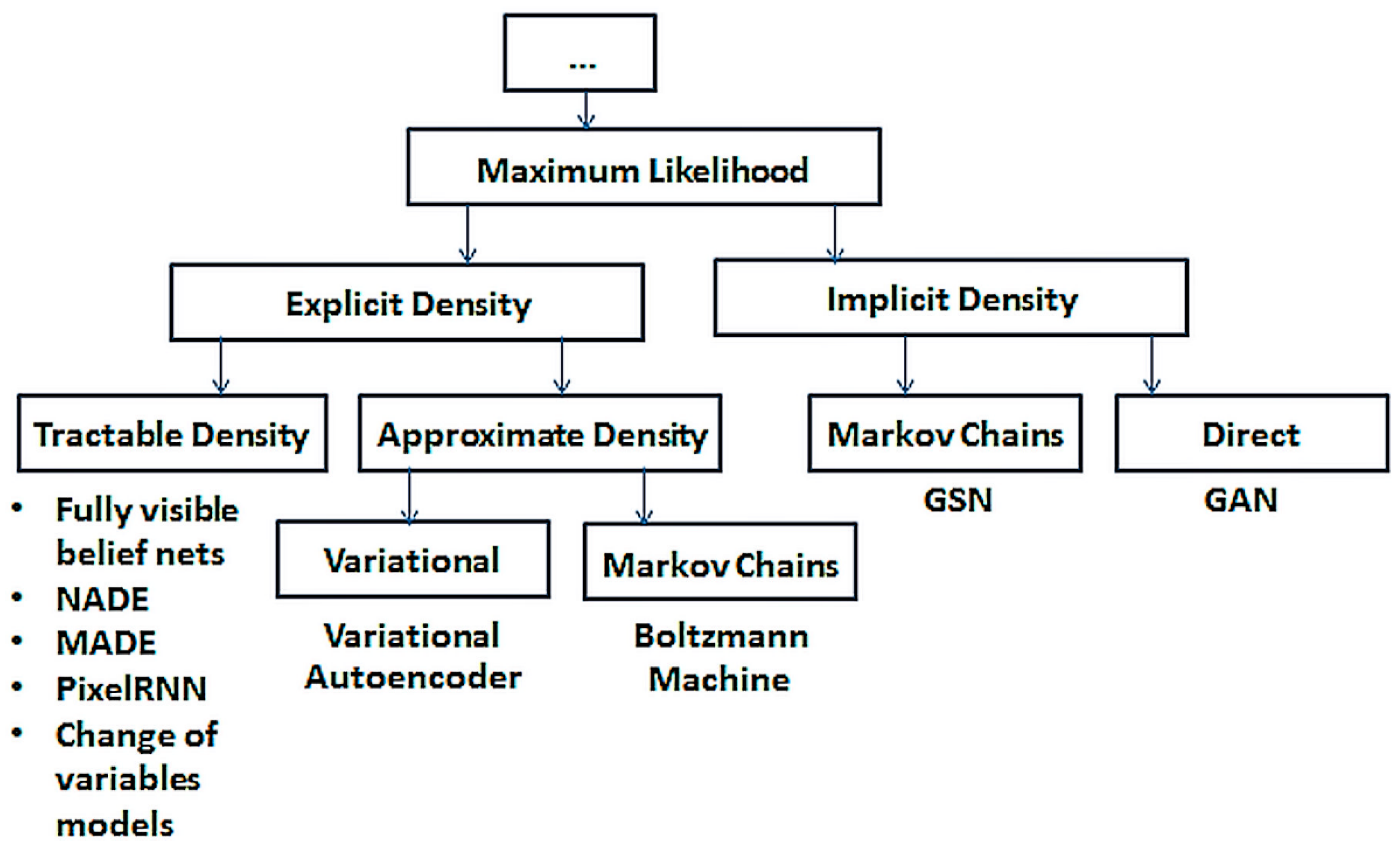
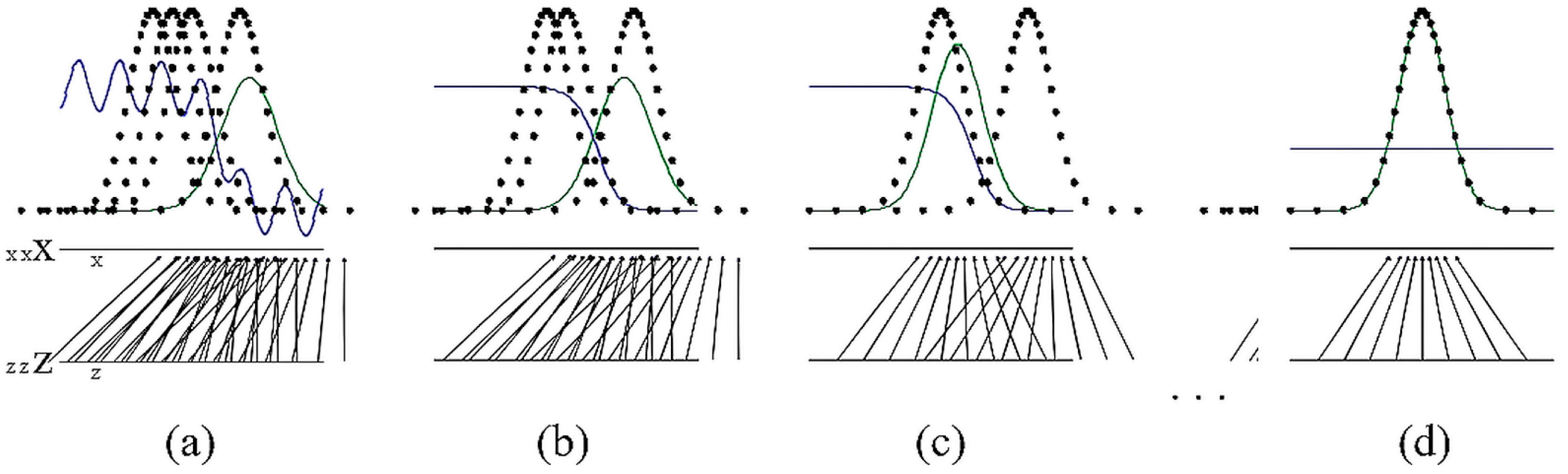
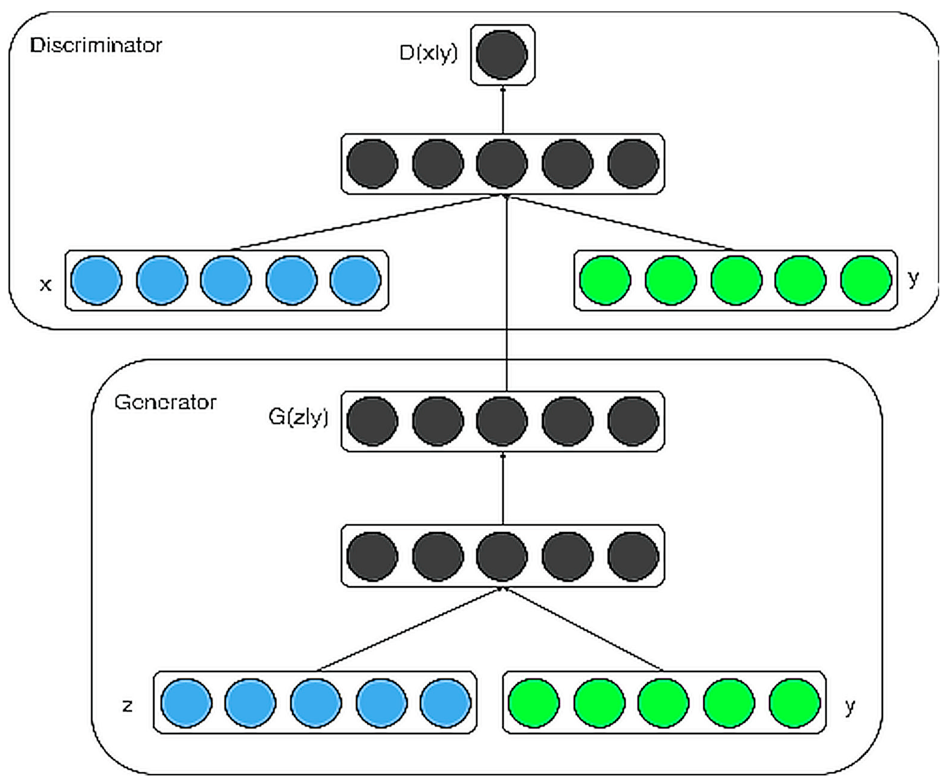
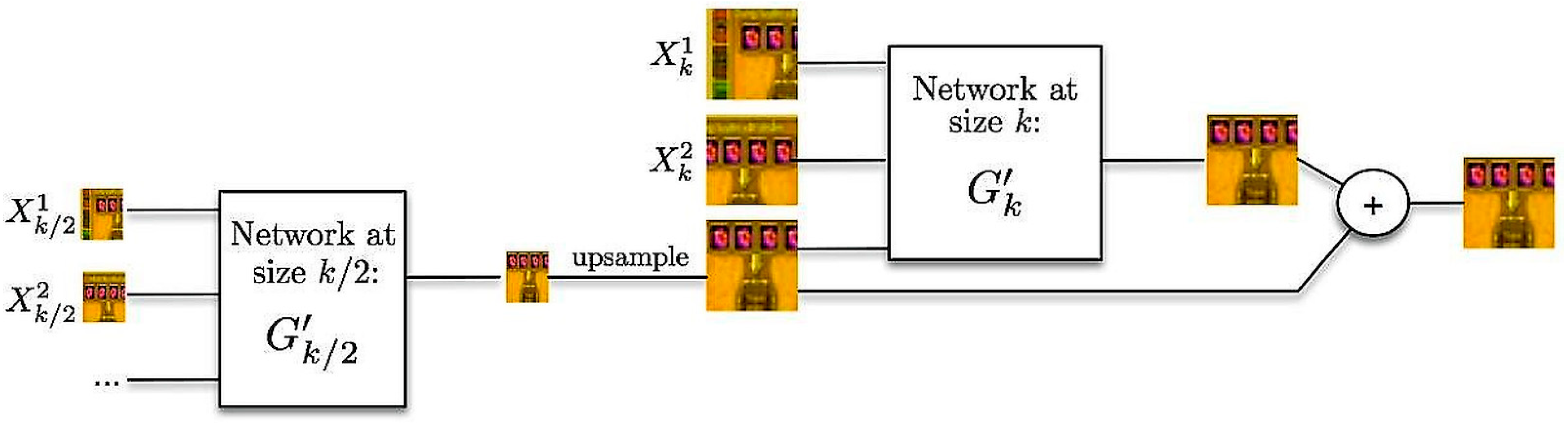
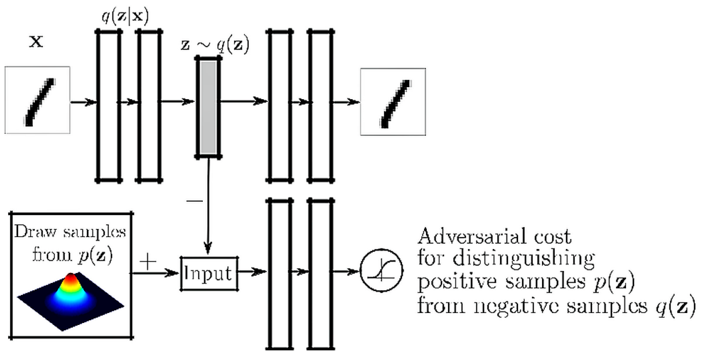
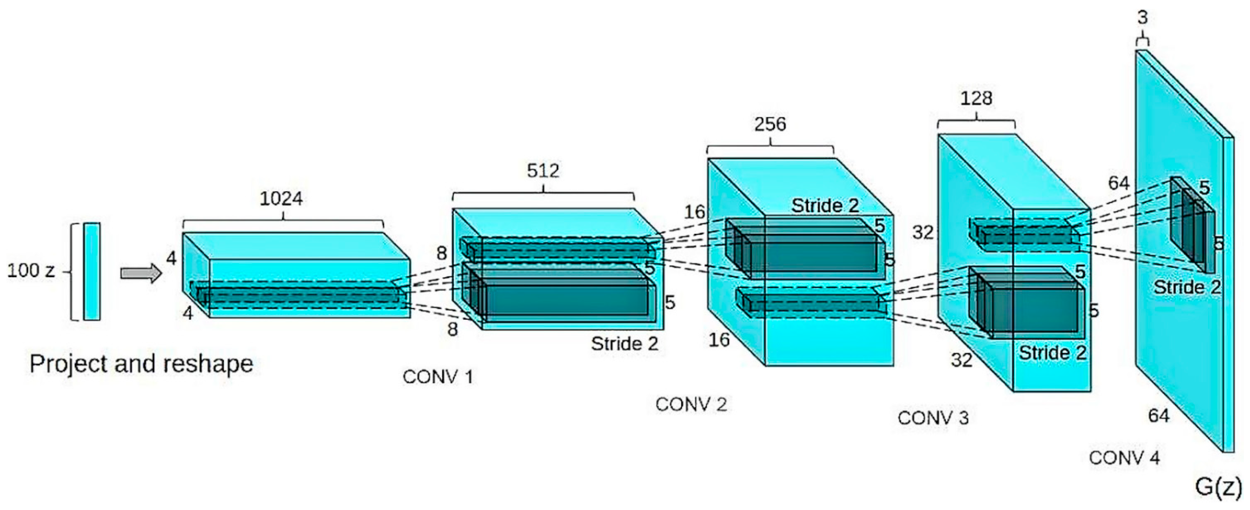
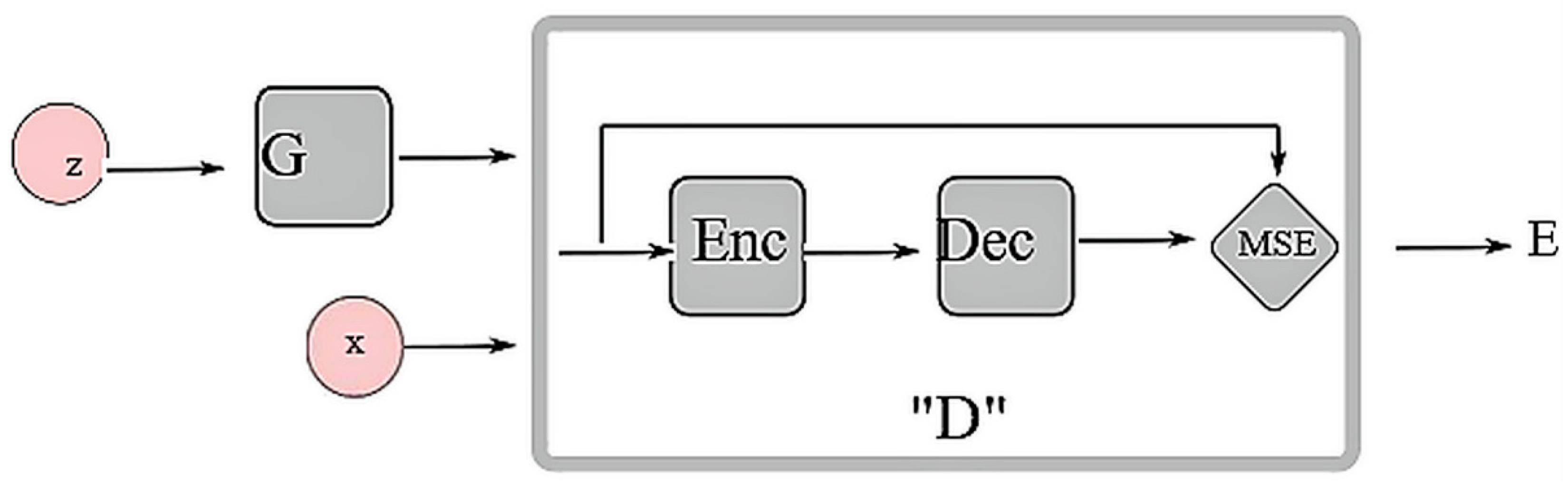
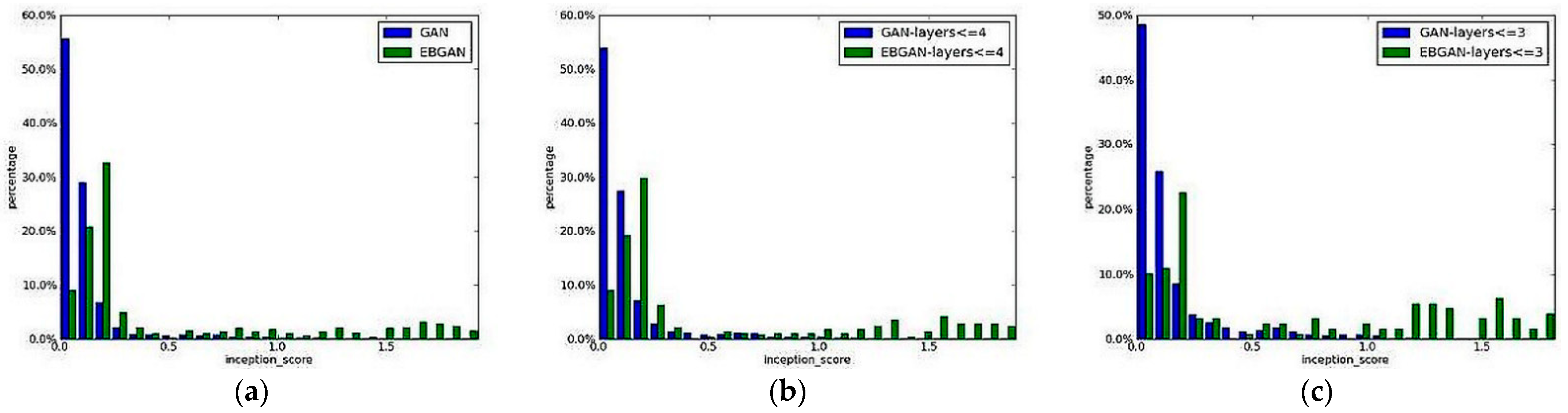
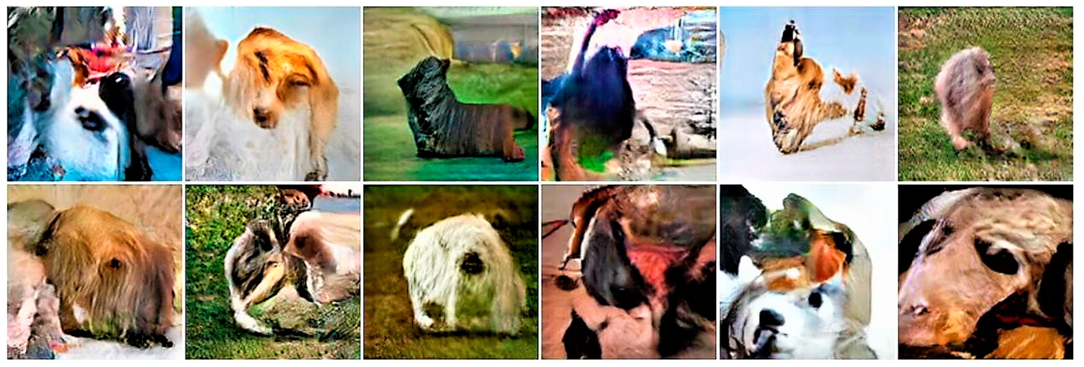
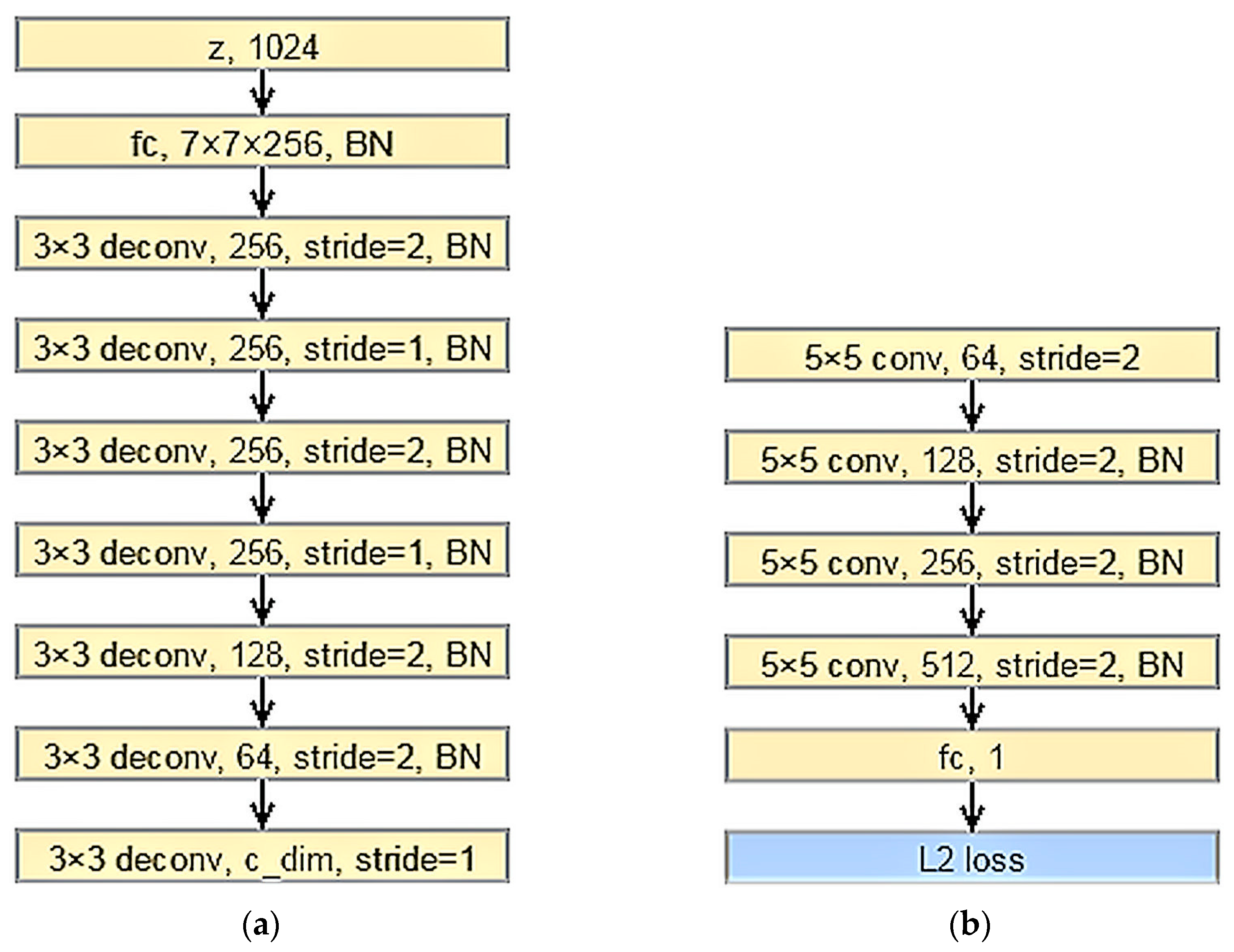
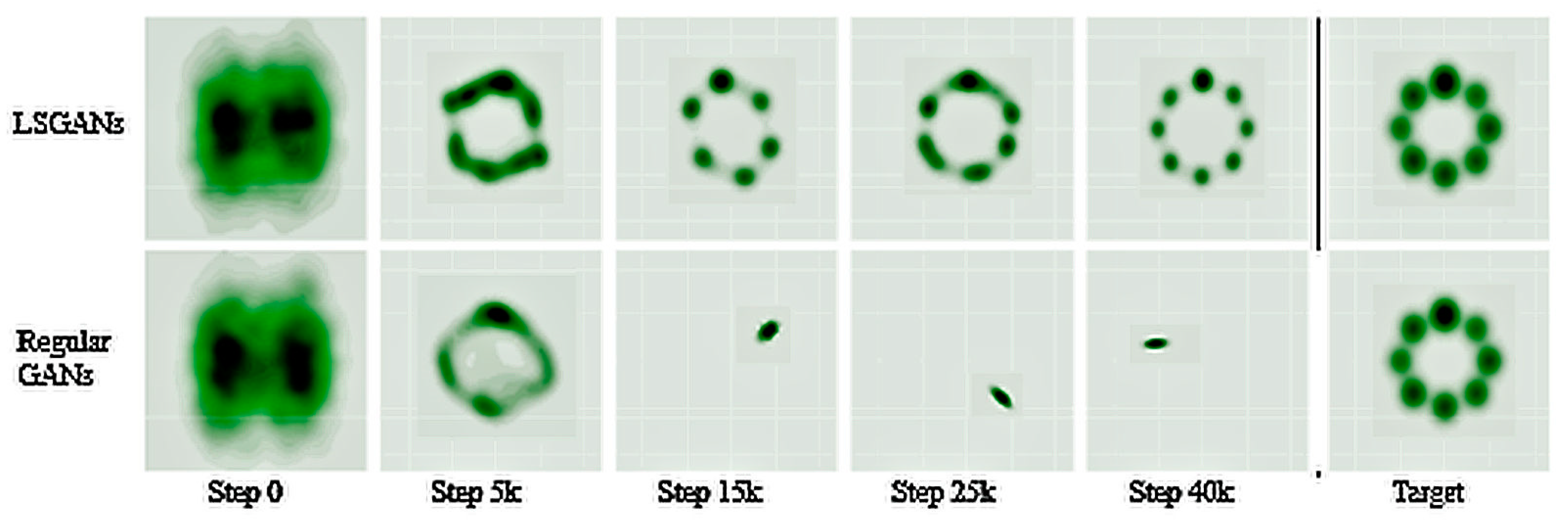
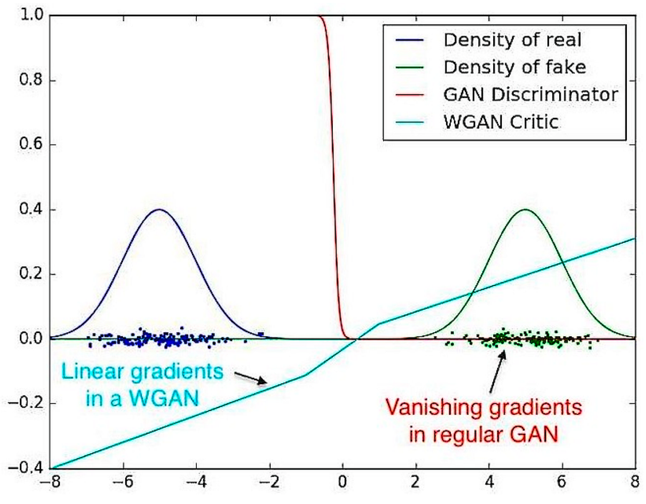
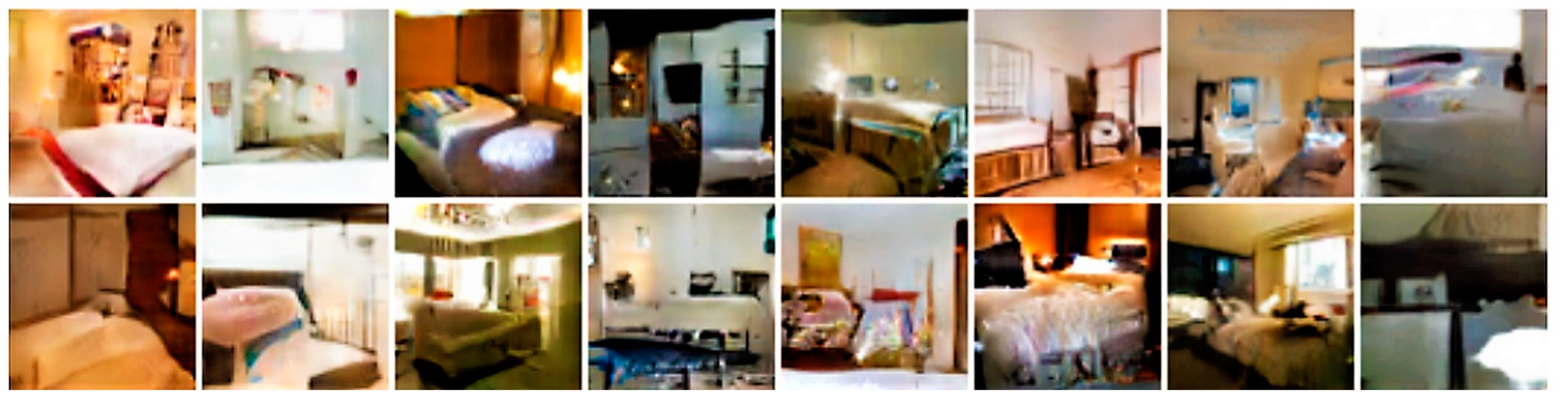
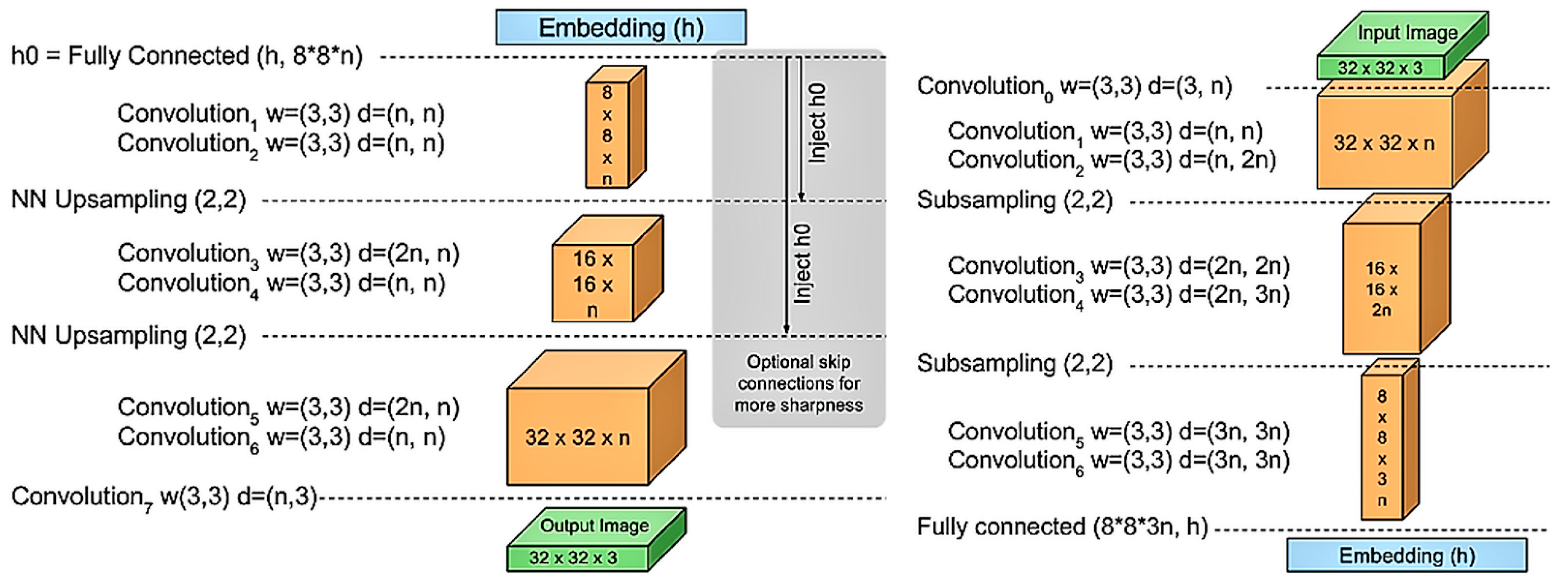
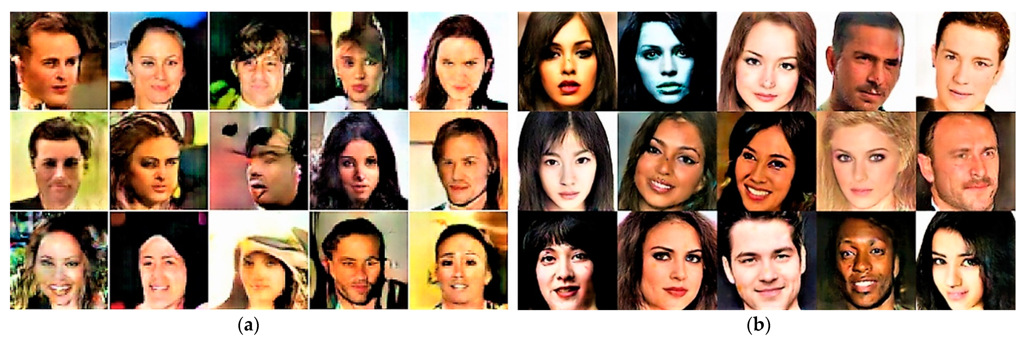
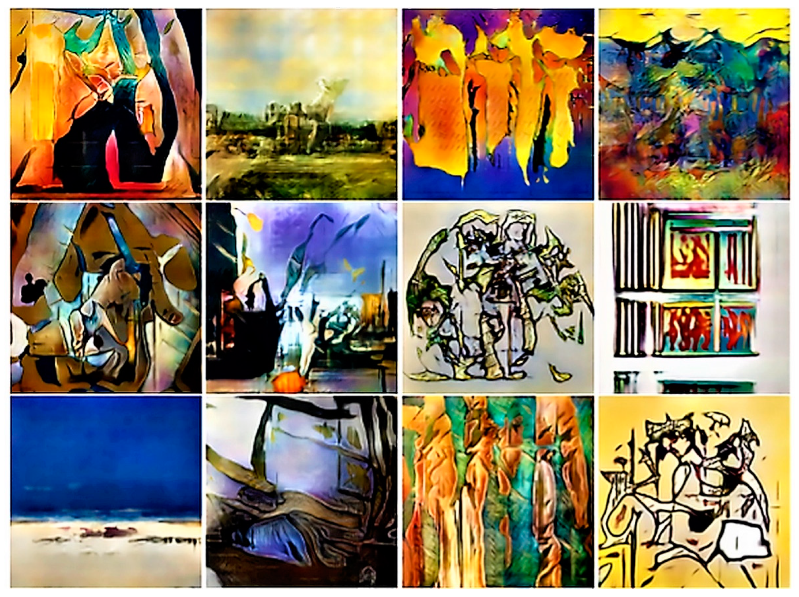
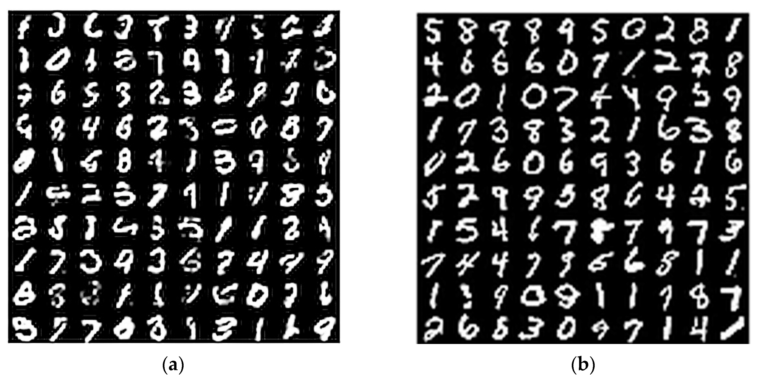
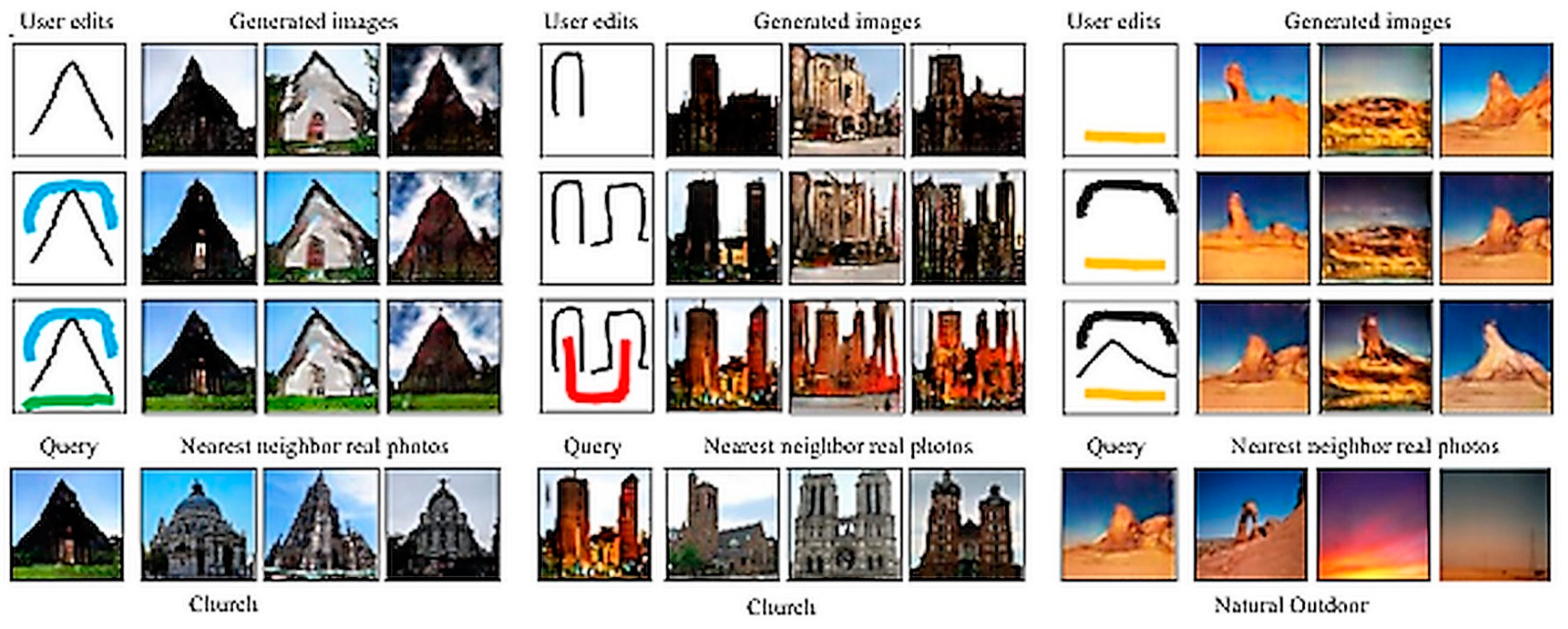
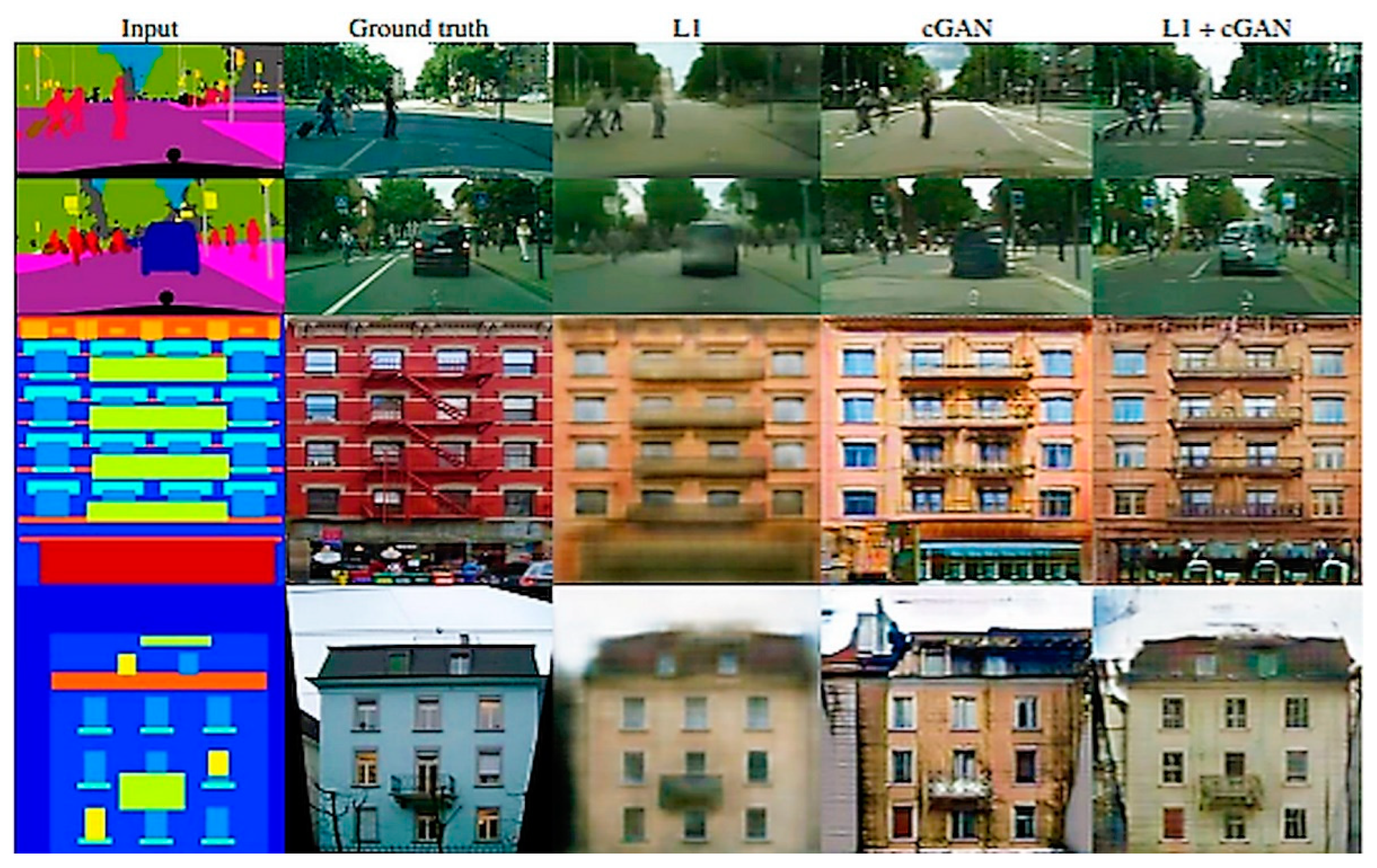
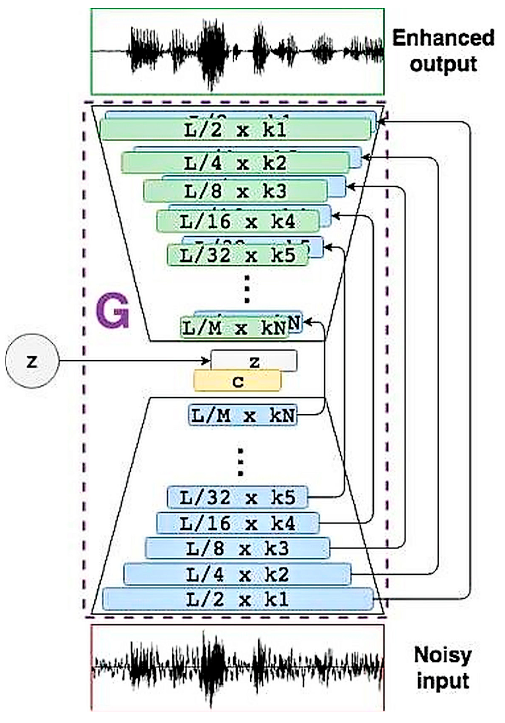
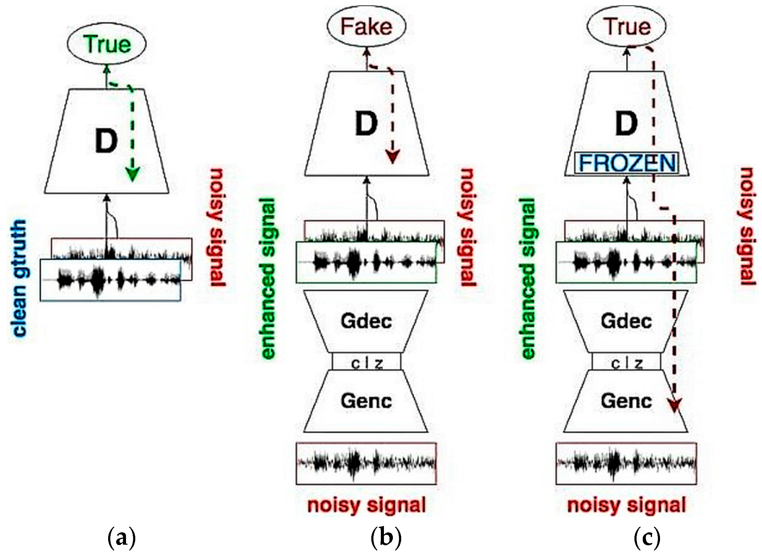
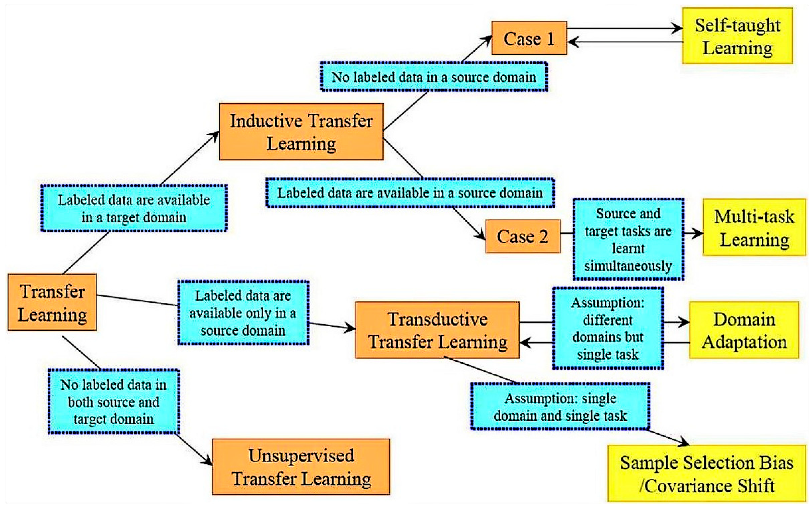
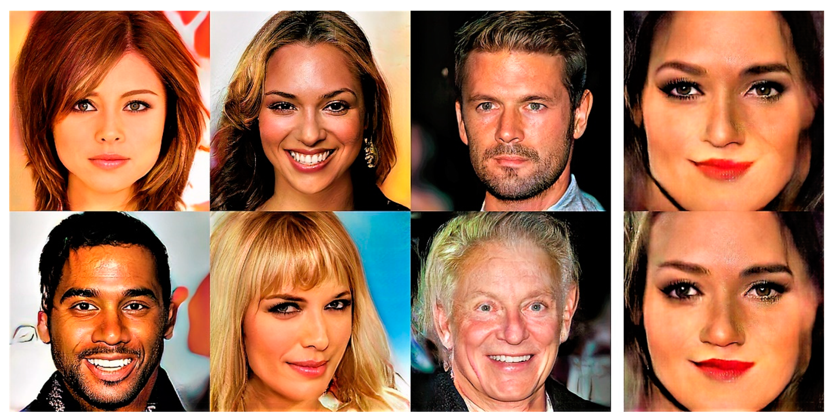
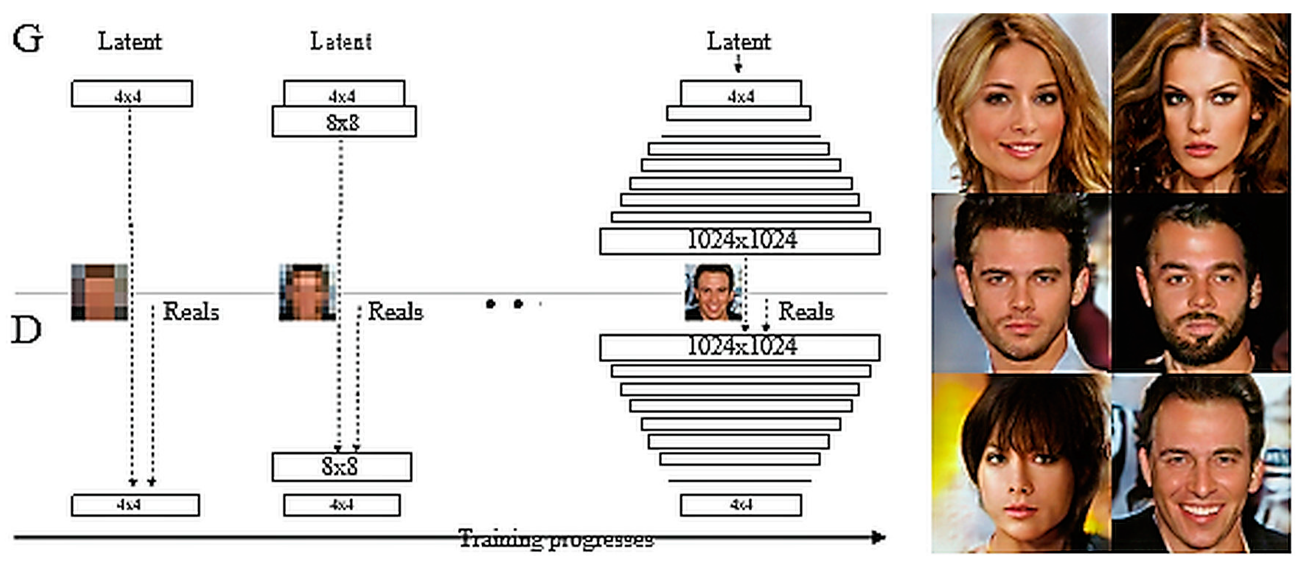
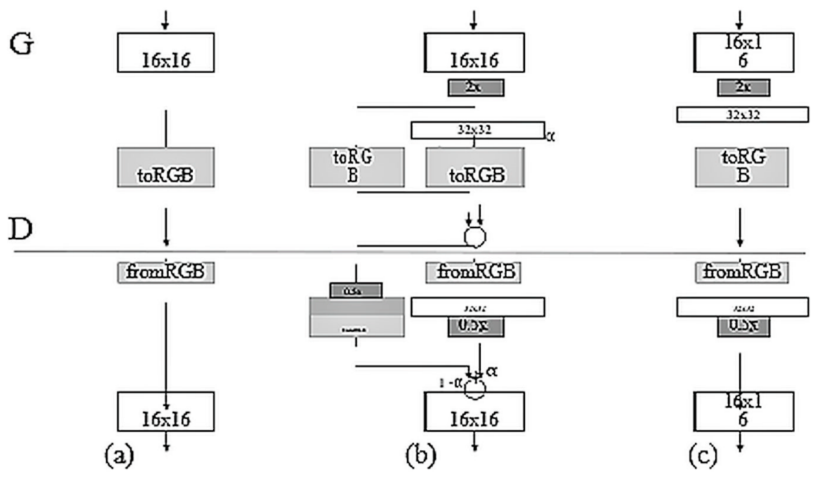
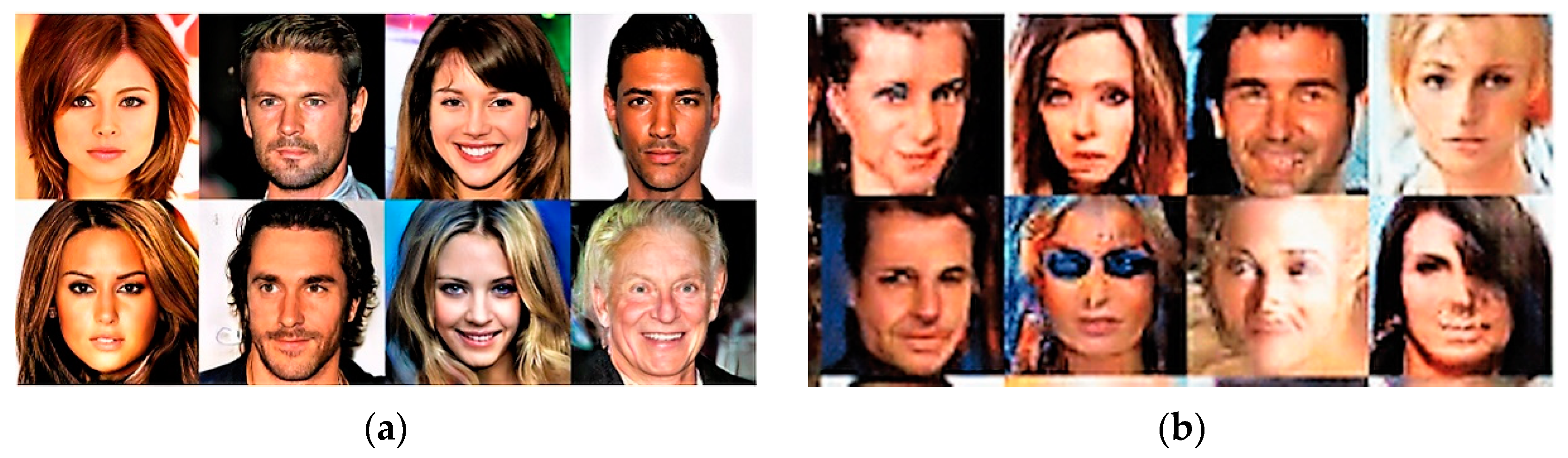