Article

Analysis of the Applicable Range of the Standard Lambertian Model to Describe the Reflection in Visible Light Communication

1
Key Laboratory of High Speed Circuit Design and EMC of Ministry of Education, School of Electronic Engineering, Xidian University, Xi’an 710071, China
2
Department of Electrical and Computer Engineering, Attock Campus, COMSATS University Islamabad, Islamabad 43600, Pakistan
*
Authors to whom correspondence should be addressed.
Electronics 2022, 11(9), 1514; https://doi.org/10.3390/electronics11091514
Submission received: 20 March 2022 / Revised: 28 April 2022 / Accepted: 5 May 2022 / Published: 9 May 2022
(This article belongs to the Section Microwave and Wireless Communications)

Abstract

:
The existing visible light communication simulation research on reflection is mainly based on the standard Lambertian model. In recent years, some papers have mentioned that the standard Lambertian model is too simplified and approximate to meet the actual situation. To solve this problem, a variety of more complex reflection models have been proposed. However, the more complex models require more computation. To balance computation and simulation accuracy, by consulting the literature, this study found that the standard Lambertian model has a certain requirement of the incident angle range to describe reflection on a wall covered in plaster. In this paper, the inappropriate index Q of the standard Lambertian model is defined, and then the relationship between Q and the light-emitting diode position with only the first reflection considered is determined through a preliminary calculation. The calculation shows that, in an empty room with plaster walls, and when the distance is greater than 0.685 m, the standard Lambertian model can be used; when the distance is less than 0.685 m, other, more complex models need to be adopted according to the actual situation.

1. Introduction

The existing visible light communication (VLC) simulation research is mainly based on two important theoretical models, the generalized Lambertian model of a light-emitting diode (LED) light source and the standard Lambertian model of a reflective surface [1,2,3,4,5]. With the improvement in computer performance and the continuous advancements in VLC research, some researchers are aware that these previous relevant works assumed some sort of simplification to evaluate the propagation channel, which might not hold true for many practical cases [6,7,8].
In [9], the Lambertian specular reflections model and the Lambert–Phong diffuse reflection model for both vertical- and angular-oriented receiver detectors were considered. In [10], Phong’s model was used to describe the reflection pattern. In [11], depending on the materials, reflection was assumed to be Lambertian or to follow the Blinn–Phong model. In [12], the integration of new reflection models into the impulse response estimation of the indoor wireless optical communication channels is proposed, including Phong’s model, retroreflective Phong’s model, Blinn’s model, and Lafortune’s model.
Complex models require more calculations. To balance computation and simulation accuracy, first, this study reviewed the related papers on the standard Lambertian model in VLC. Second, the inappropriate index Q of the standard Lambertian model was defined. Then, based on [1], in which the standard Lambertian model was first applied to optical communication to describe reflection, calculations of the relationship between the Q and the position of the LED in some different situations with only the first reflection considered were performed. Finally, by analyzing the calculation results, the applicable range of the standard Lambertian model to describe the reflection of an empty room with plaster walls in VLC was obtained.
Based on the above discussion, the contributions of this paper are as follows:
  • The inappropriate index Q of the standard Lambertian model is defined for the first time;
  • The relationship between the Q and the position of the LED is simulated in some different situations with only the first reflection considered;
  • The range of LED positions, for which the standard Lambertian models can be used to describe the reflection of an empty room with plaster walls applicably, is determined.
Following the introduction, this paper is organized into four sections. In Section 2, the application scope of the standard Lambertian model in the original paper is explained. In Section 3, the inappropriate index Q of the standard Lambertian model is defined, and then three simplified situations—one infinitely long wall, a corner between two infinitely long walls, and a square empty room with an LED installed in the center of the ceiling—are used to simulate and analyze the relationship between the Q and the LED position. In Section 4, the relationship between the Q and the LED position in differently sized rooms is simulated and analyzed. Finally, our conclusions are given in Section 5.

2. Standard Lambertian Model

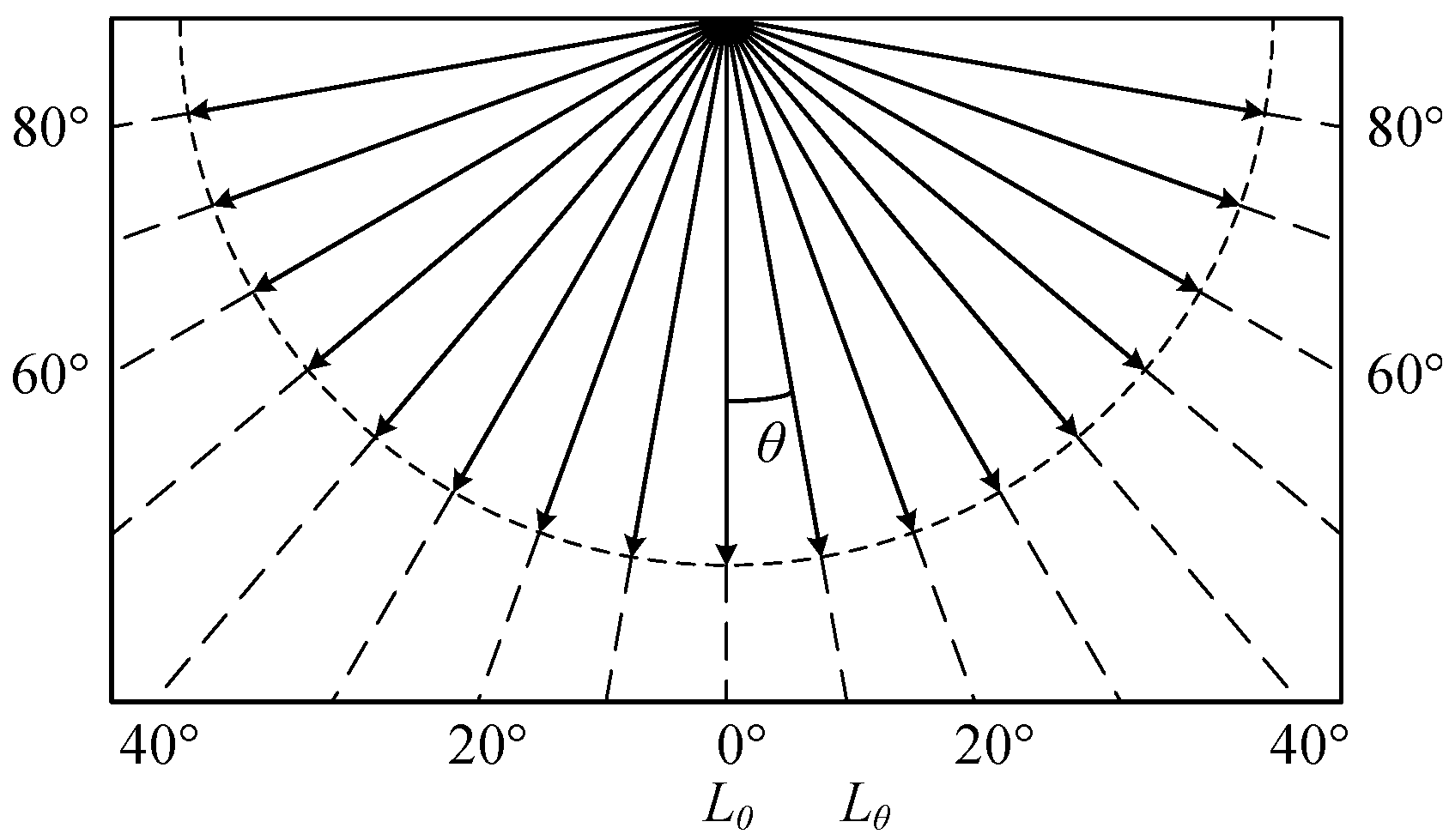
2.1. Definition of the Standard Lambertian Model

The standard Lambertian light source (Lambertian body, Lambertian surface) is an ideal light source model in which luminous intensity conforms to the law of cosines, as shown in Figure 1. In this model, the luminous intensity along one orientation (Iθ) is equal to the cosine of the angle between the orientation and the optical axis (θ) multiplied by the luminous intensity along the optical axis (I0), in candela units (cd) [13], as follows:
I θ = I 0 cos θ
where Iθ is the luminous intensity along the orientation with the θ angle between the optical axes; θ is the angle between the orientation and the optical axes; I0 is the luminous intensity along the optical axes.
Figure 2, a normalized luminance distribution diagram, shows that the luminance in candelas per square meter (cd/m2) of the standard Lambertian light source is independent of orientation [13], as follows:
L θ = d I θ d S = d I 0 cos θ d A cos θ = I 0 d A
where dS is the surface element of the light beam cross-section; dA is the surface element of the luminous surface; θ is the angle between the normal dA and the light beam direction.
Due to the fact that the luminance of the standard Lambertian light source is independent of direction, the standard Lambertian surface is regarded as an ideal diffuse reflection surface [14,15].

2.2. Origin of the Standard Lambertian Model in VLC

In [1], the standard Lambertian model is first introduced into optical communication reach, and some important conclusions in it are as follows:
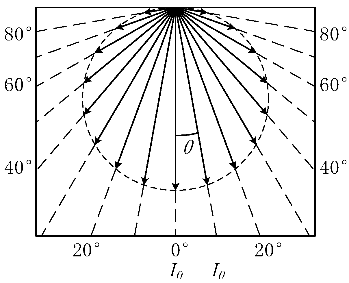
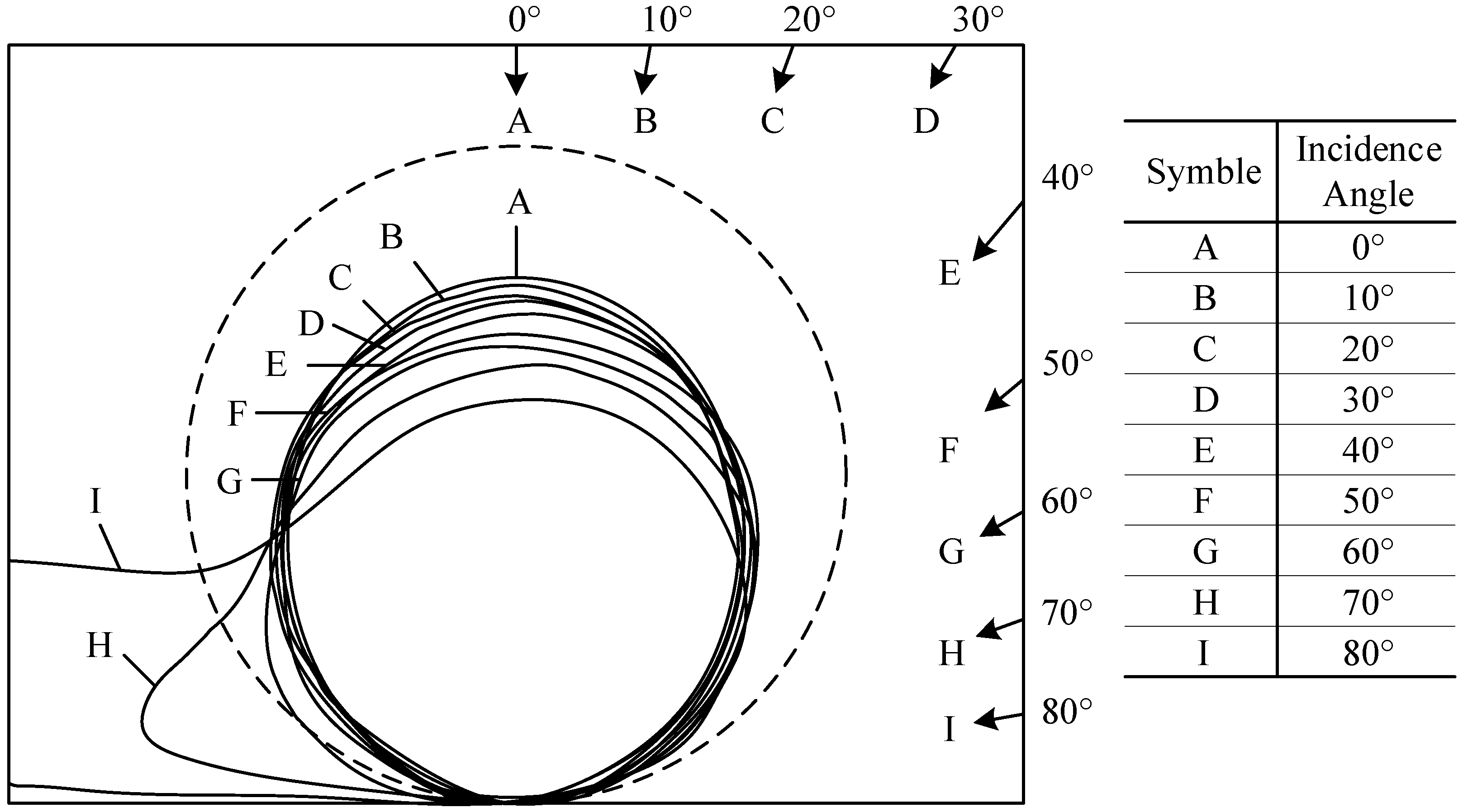
  • Using an infrared light with a wavelength of 950 nm to measure the reflected luminous intensity distribution of a white plaster wall, Figure 3 was drawn, where the letters indicate the incident angle, and the dotted circle is the luminous intensity distribution characteristic diagram of the standard Lambertian surface;
  • The reflection characteristics are generally composed of a diffuse and a specular component, the latter becoming significant with very shallow angles of the incident radiation;
  • Typical values of the reflection coefficient for plaster walls vary between 0.7 and 0.85 depending on the surface texture and angle of incidence, and the radiation characteristics are a close fit to a Lambertian distribution.
Professor Masao Nakagawa of Japan started the research on VLC early, and his published paper [2] cited the standard Lambertian model in [1], which is the most cited paper in this field, to introduce the standard Lambertian model to VLC.

3. Simplified Analysis

In this paper, relative attenuation was adopted as the inappropriate index Q, in dB units, of the standard Lambertian model, as follows:
Q = 10 lg F n o L F L
where Fno−L is the luminous flux of the reflected light not in the standard Lambertian model, namely the luminous flux of the part with the incident angle greater than 70°, according to Figure 3; FL is the luminous flux of the reflected light in the standard Lambertian model, namely the luminous flux at an incident angle of less than or equal to 70°, according to Figure 3. Both Fno−L and FL are shown in lumens (lm).
The larger the Q is, the larger the proportion of the luminous flux of the reflected light not in the standard Lambertian model to the total luminous flux reflected. In this case, the inappropriateness of the standard Lambertian model is higher, and the model cannot fit the actual situation well. On the contrary, the smaller the Q is, the smaller the proportion of the luminous flux of the reflected light not in the standard Lambertian model to the total luminous flux reflected. Similarly, the inappropriateness of the standard Lambertian model is lower, and the model can fit the actual situation well.
This section is divided into three parts. The relationship between the Q and the LED position was simulated and analyzed under three different simplified situations—one infinitely long wall, a corner between two infinitely long walls, and a square empty room with an LED installed in the center of the ceiling.

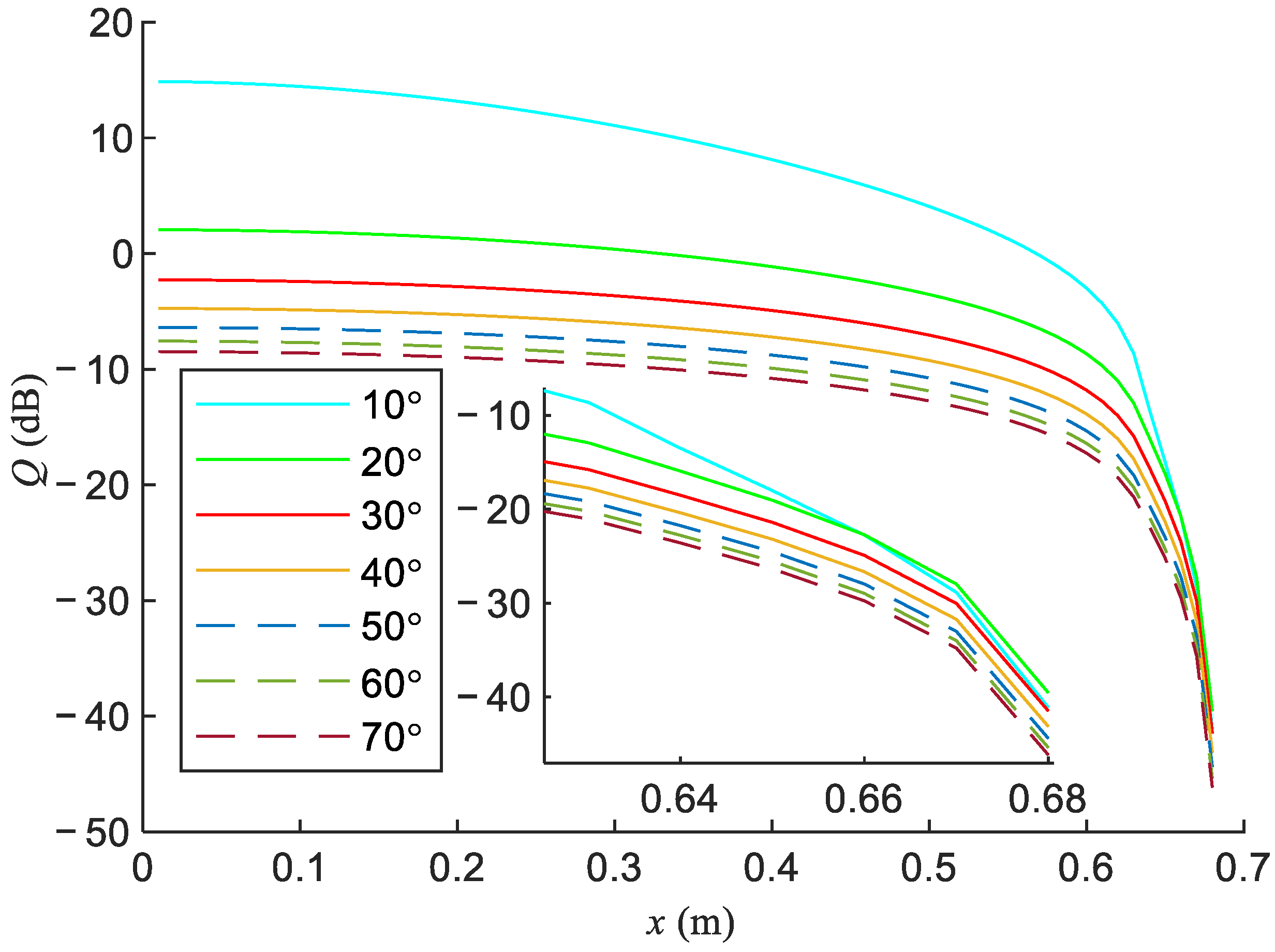
3.1. One Infinitely Long Wall

3.1.1. Situation Description

In the situation of one infinitely long wall, the LED installation position and the calculation analysis of the inappropriate standard Lambertian model are shown in Figure 4. The LED installation height hLED was 2.5 m and the luminous surface was placed horizontally downward. The height of the receiving plane hr was 0.75 m, and the receiving surface was placed horizontally upward. In Figure 4, the line area was a half cone, with the LED as the vertex, the wall as the bottom, and a 70° cone half-angle. In the half cone, the incident angle of any light emitted from the LED to the wall was less than or equal to 70°, so the luminous flux reaching the line area on the wall was reflected in the standard Lambertian model. Since only the first reflection was considered in this calculation and the receiver was placed horizontally upward, it was impossible for the wall area below the height of the receiving plane to reach the receiving area after a reflection. Therefore, the luminous flux above the height of the receiving plane and outside the line area was not reflected in the Lambertian model. The distance x between the LED and the wall was the independent variable. Appendix A shows the specific calculation formulas.

3.1.2. Calculation Setting

Table 1 shows the calculation settings for all three situations. According to Equation (3), the calculation results are independent of the axial luminous intensity of the LED. However, based on the needs of the calculations, the axial luminous intensity of the LED is consistent with that in [2].

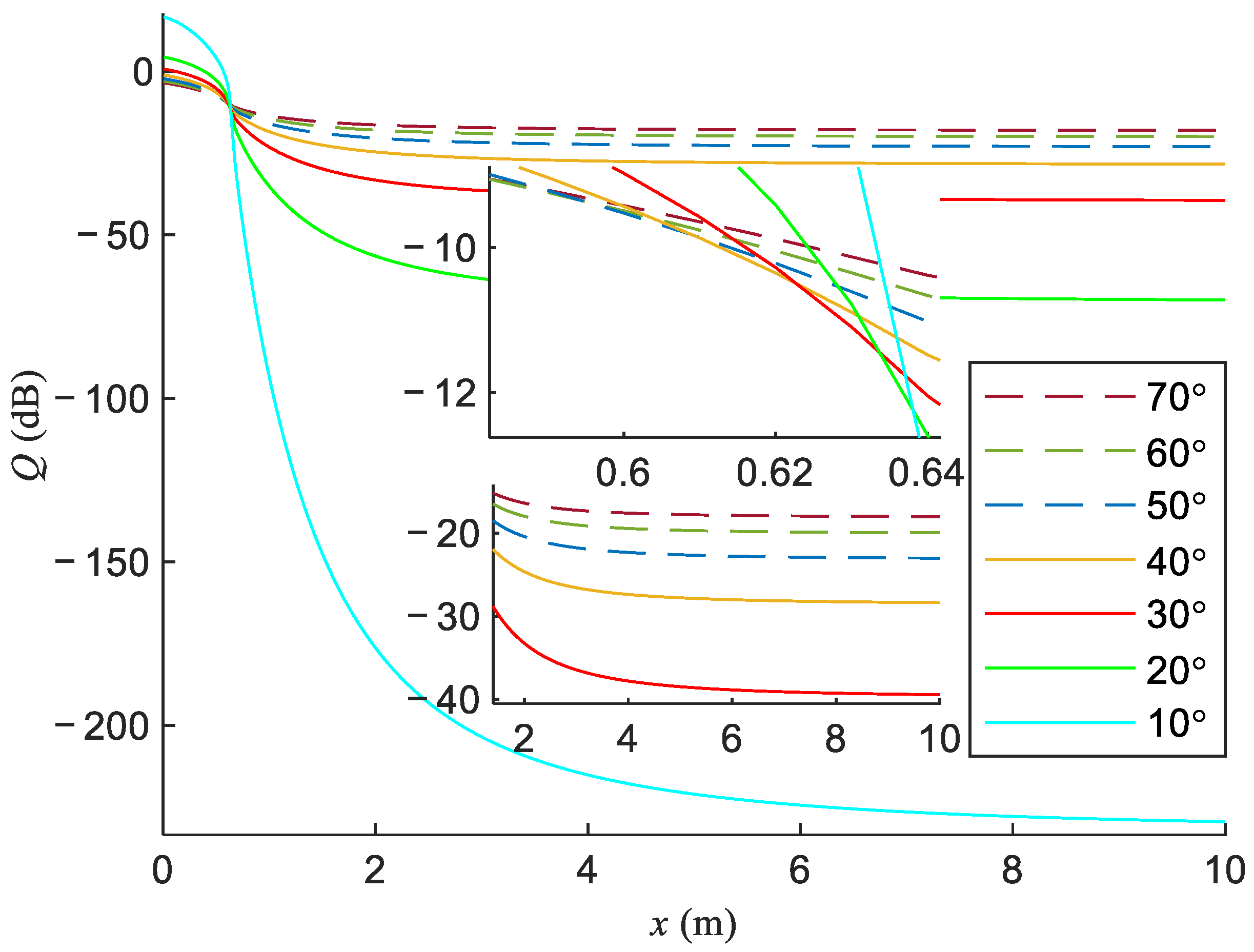
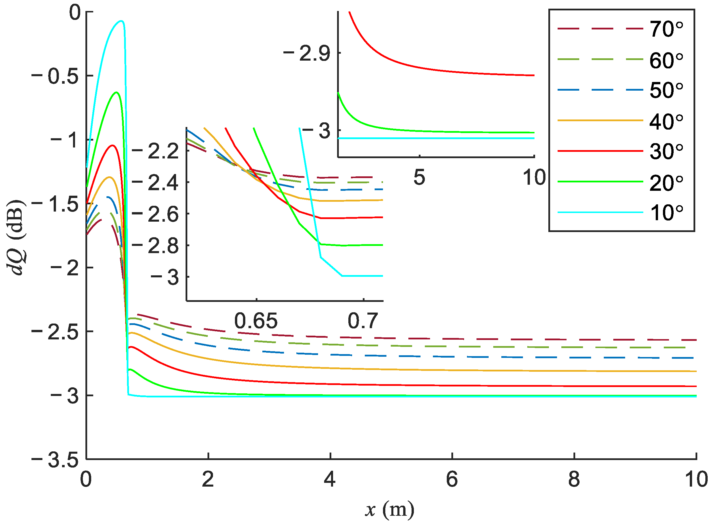
3.1.3. Calculation Results

Figure 5 shows the calculation results of the relationship between the Q and x in the situation of one infinitely long wall. According to Figure 5, when the LED was close to the wall, the Q was high, and the standard Lambertian model was not applicable. The Q decreased as the distance x increased, and the downward trend of the Q first increased and then decreased as x increased. The larger the semi-luminous intensity angle was, the smaller the initial value of the Q was, and the more gentle the change in the Q was, the earlier it entered the stabilization stage and the larger the Q was at the stabilization stage.

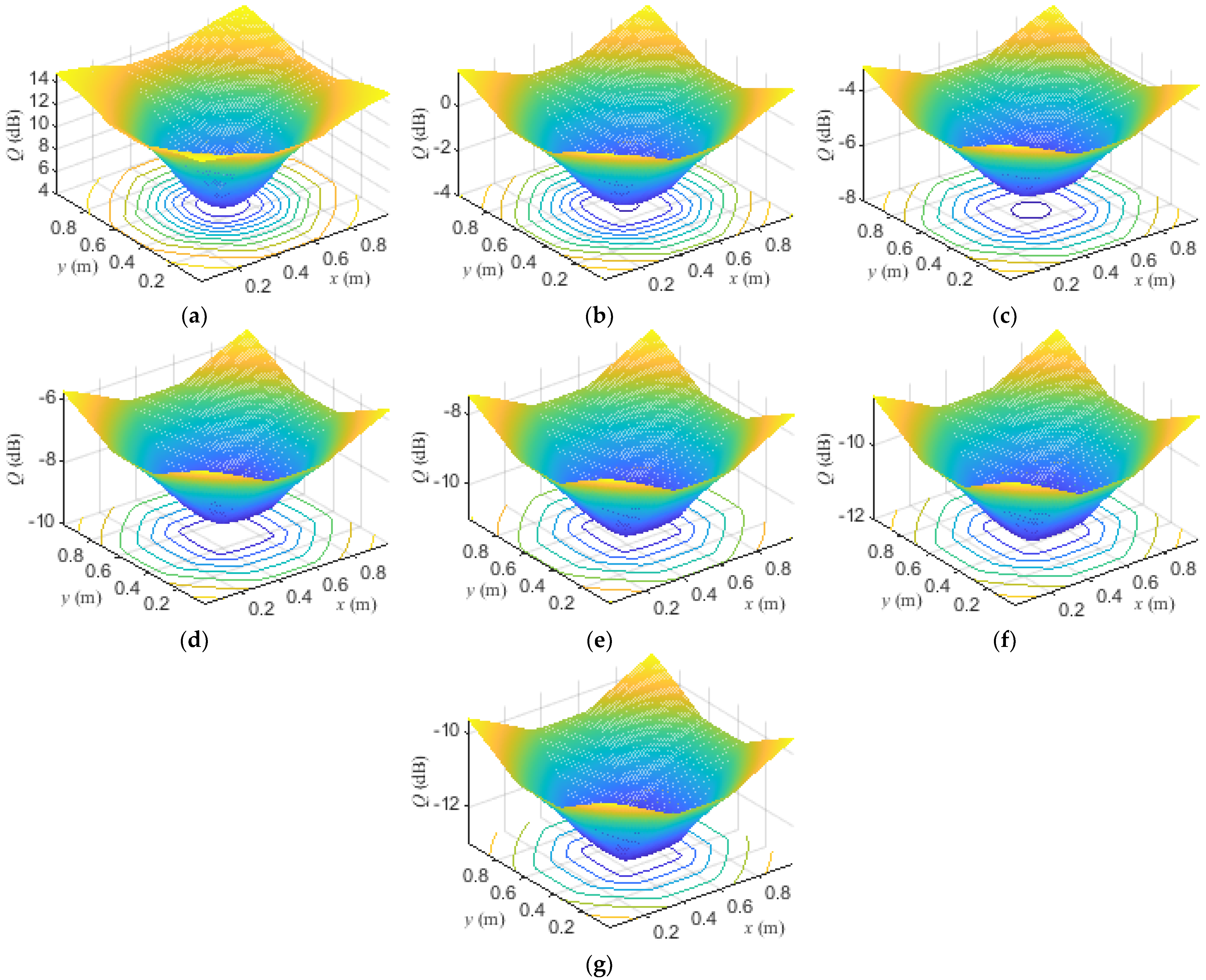
3.2. A Corner between Two Infinitely Long Walls

3.2.1. Situation Description

In the situation of a corner between two infinitely long walls, the LED installation position and the calculation analysis of the inappropriateness of the standard Lambertian model are shown in Figure 6. In Figure 6, the line area is composed of two half cones with the LED as the vertex, the wall as the bottom, and a 70° cone half-angle. In the two-half-cone complex, the incident angle of any light emitted from the LED to the wall was less than or equal to 70°, so the luminous flux reaching the line area on the wall was reflected in the standard Lambertian model. The LED was installed on the bisector of the angle between the two walls on the ceiling. The other settings were the same as in Section 3.1. Appendix B shows the specific calculation formulas.

3.2.2. Calculation Results

Figure 7 shows the calculation results of the relationship between the Q and x in the situation of a corner between two infinitely long walls. In comparing Figure 7 with Figure 5, it can be found that all the features in Figure 5 are also reflected in Figure 7. Figure 8 is the result of subtracting the Q in Figure 5 from the data in Figure 7. It can be found that the Q of Section 3.2 was lower than that of Section 3.1, and the difference first decreased and then increased with the increase in distance. When the distance reached a certain level, the difference basically remained unchanged.

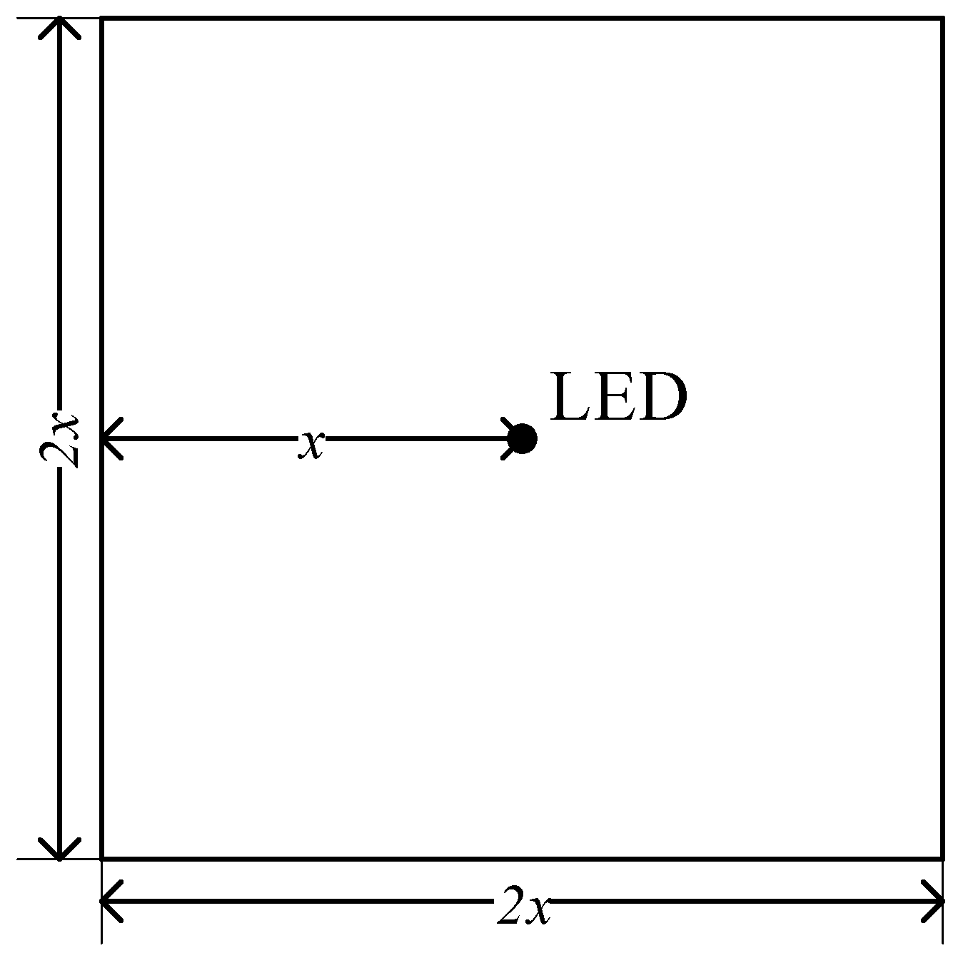
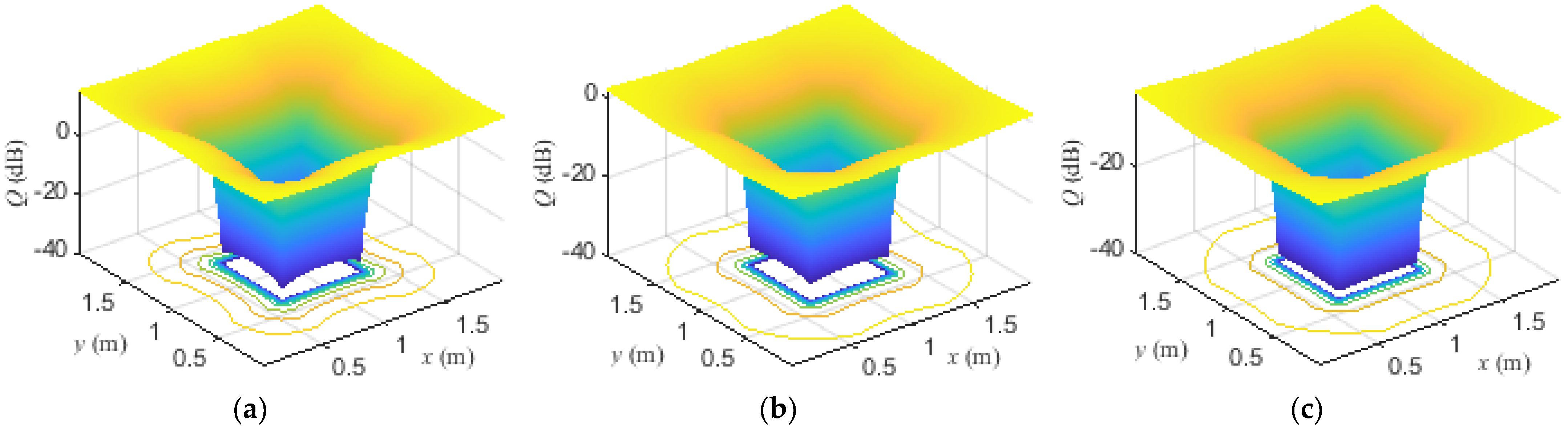
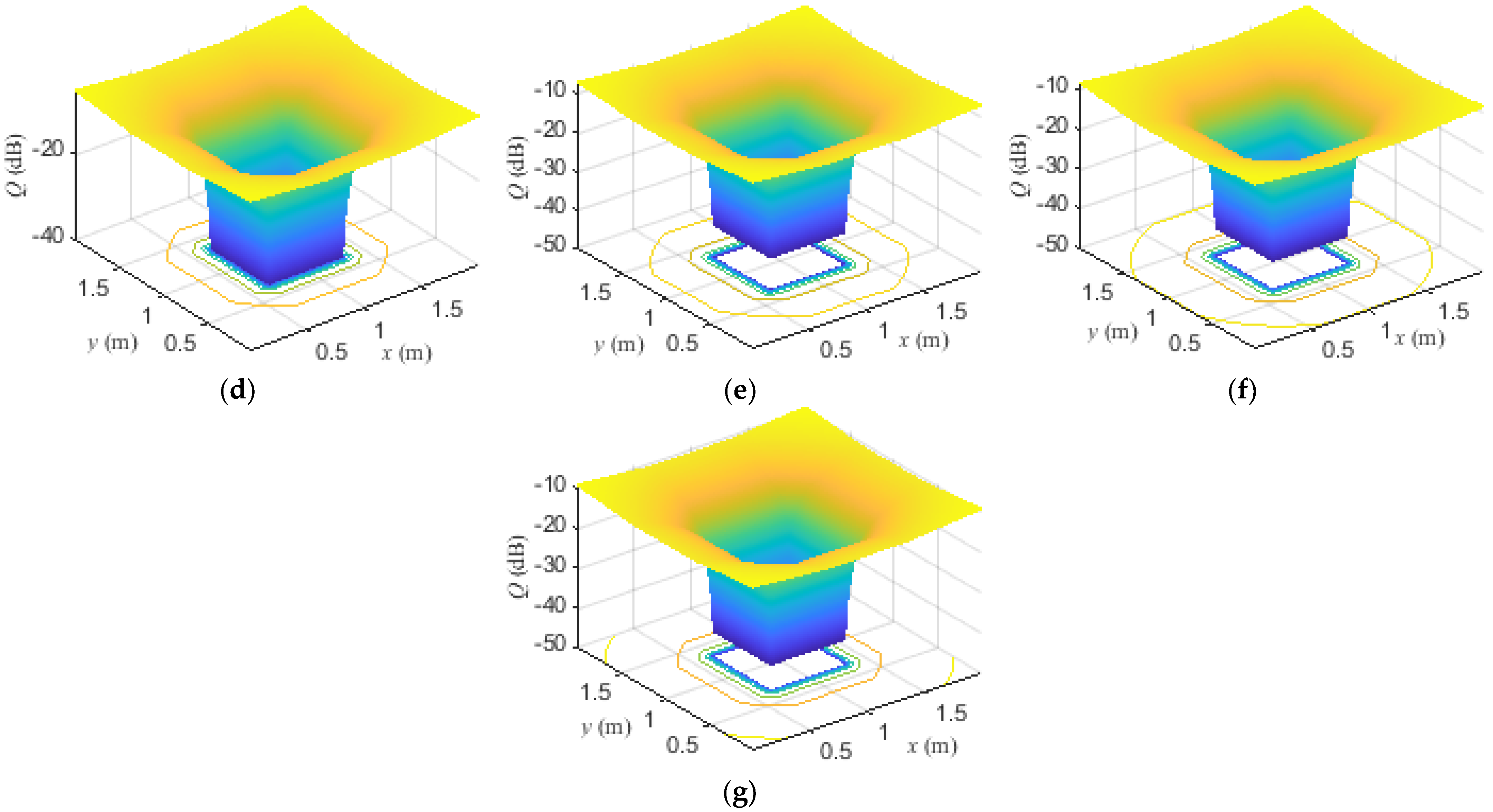
3.3. A Square Empty Room with an LED Installed in the Center of the Ceiling

3.3.1. Situation Description

The LED installation position in this situation is shown in Figure 9. An LED was installed in the center of the ceiling, and the length and width of the room were equal. Appendix C shows the specific calculation formulas.

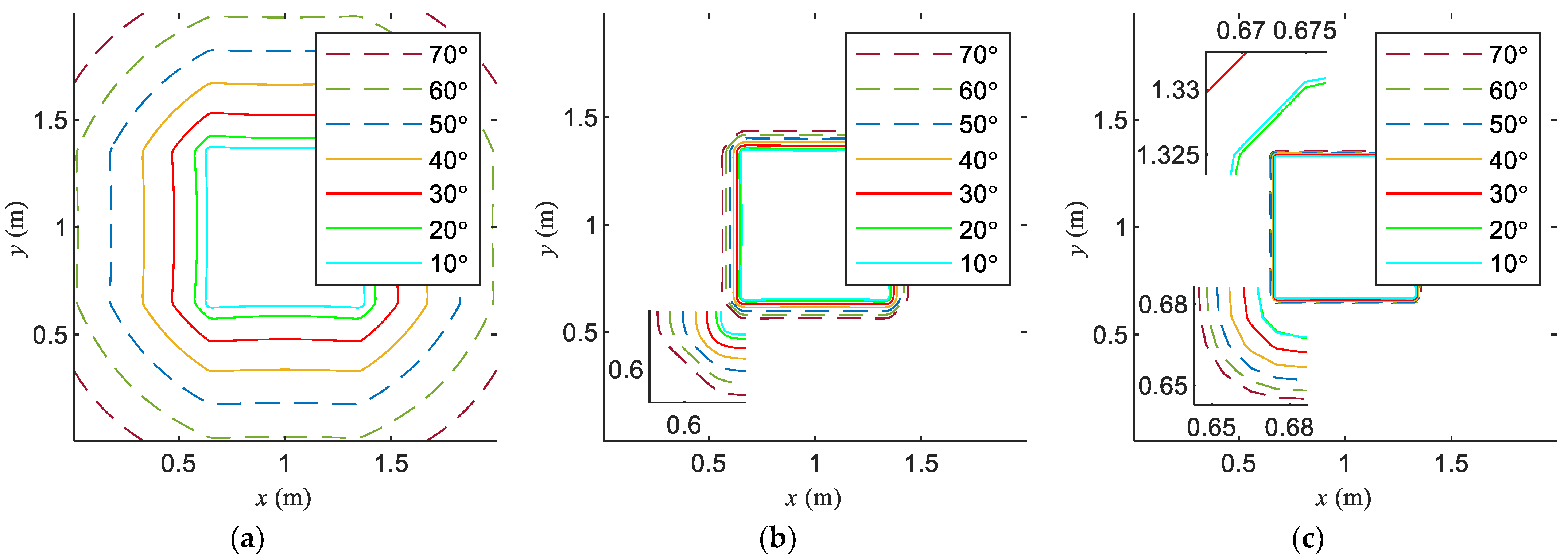
3.3.2. Calculation Results

Figure 10 shows the calculation results of the relationship between the Q and x in the situation of a square empty room with an LED installed in the center of the ceiling. According to Figure 10, the Q decreased as the distance x increased, and the downward trend of Q increased as x increased. When the x reached 0.69 m, the Q was reduced to minus infinity, that is, in this case, Fno−L was 0 lm when the distance between the LED and the wall was 0.69 m or greater. After the calculation, the Q was minus infinity, when the distance between the LED and the wall was greater than 0.6839 m; this distance is denoted as xmin. Appendix C shows the specific calculation formulas.

4. Detailed Analysis

In this section, more practical and specific situations are considered, and the calculation settings in Section 3 are extended to an actual rectangular room. The scope of the LED position consideration traversed the whole ceiling, that is, the entire possible installation area was simulated and analyzed to explore the relationship between the Q and the LED position.

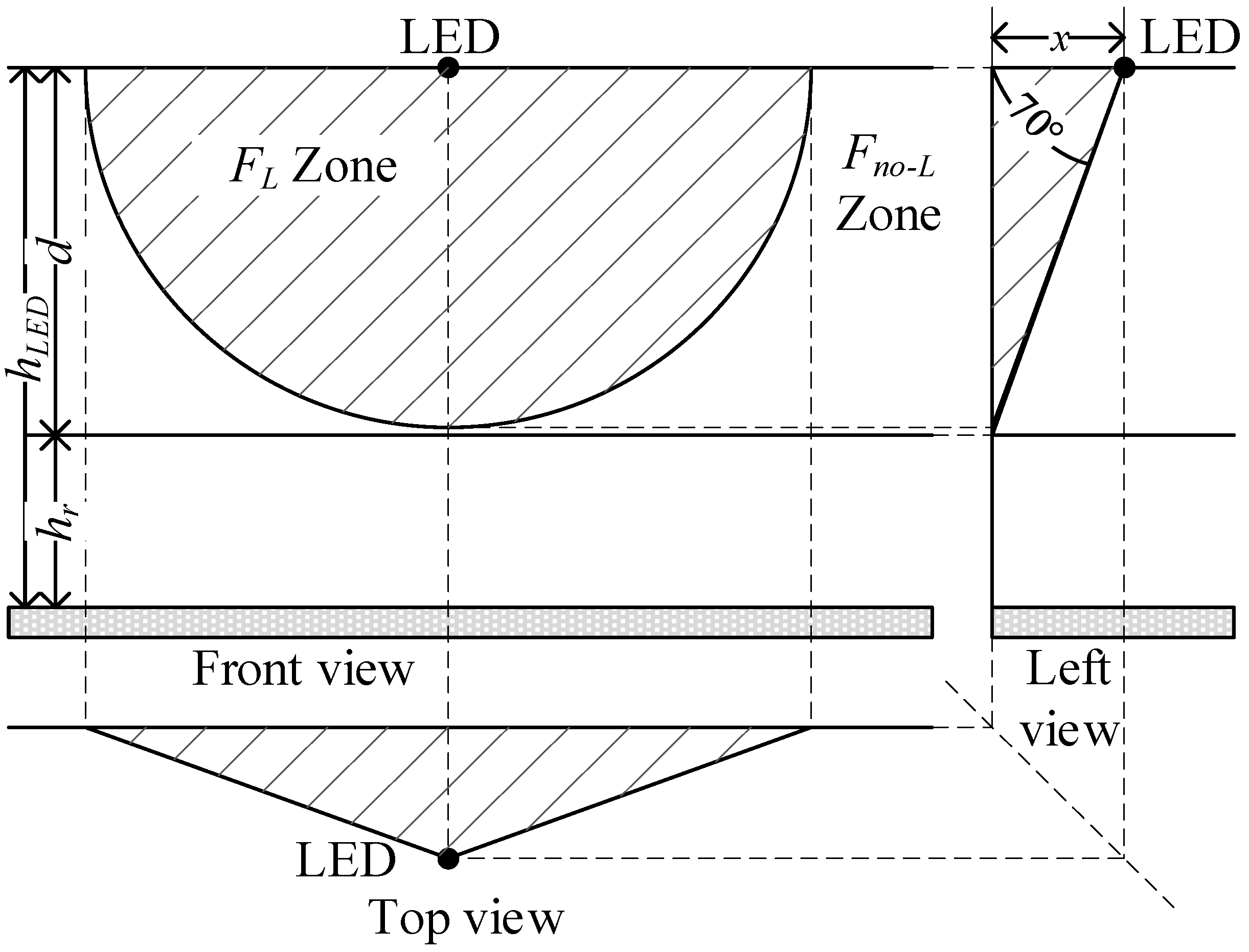
4.1. Situation Description

The calculation situation in this section is more complex than that in Section 3, but it can loosely refer to Section 3. Appendix D shows the specific calculation formulas.

4.2. Calculation Setting

All parameters were the same as in Table 1, except for the room size and the LED calculation area. Regarding the room size, we considered a variety of scenarios, the LED calculation areas were throughout the ceilings of each room, and the grid spacing was set to 1 cm.

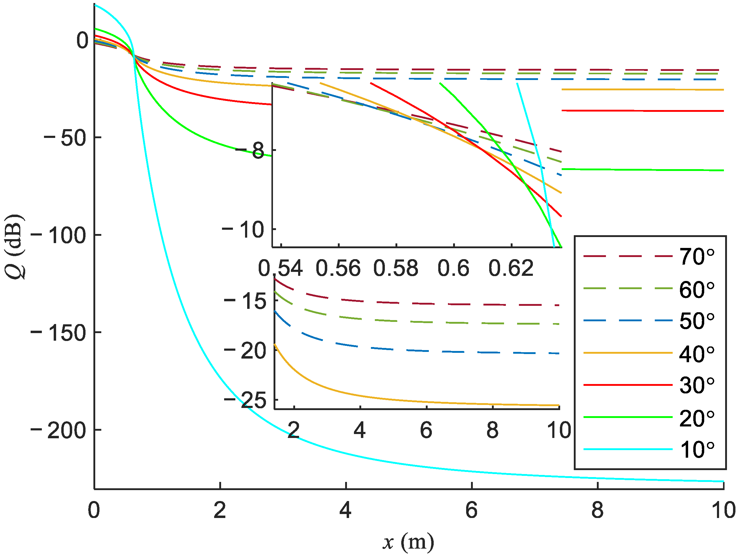
4.3. Calculation Results

Figure 11 shows the calculation results of the relationship between the Q and LED position at a room size of 1 m × 1 m. According to Figure 11, because the room size was too small, the distance between the LED and the wall was less than xmin, so there was no area where the Q was minus infinity, and the overall Q was high.
Figure 12 shows the calculation results of the relationship between the Q and LED position in a room size of 2 m × 2 m. According to Figure 12, as the size of the room was greater than 2xmin, a region with a minus infinity Q appeared in the center, and the distance between the edge of the region and the wall was 0.685 m, which is larger than and the closest to the xmin in the mesh used in the calculation.
According to the calculation results in Figure 12, the distance between the edge of the region with a minus infinity Q and the wall boundary was 0.685 m, but when the room size or the θ1/2 of the LED were different, the corresponding curves of the same Q value were different. Figure 13 shows the contour maps with Q values of −10 dB, −20 dB, and −30 dB, respectively, with the 2 m × 2 m room. Combined with Figure 12, it can be seen that the Q inside the contour line was less than or equal to the corresponding Q of the contour line. When the Q was high, θ1/2 had a greater effect on the region, but as the Q decreased, the regions corresponding to θ1/2 were close to the region with a minus infinity.

5. Conclusions

From [1], it was found that the standard Lambertian model had a certain requirement for the incident angle range to describe reflection on a wall covered in plaster. Next, the boundaries θL,Max in an incident angle domain were determined as 70°. When the incident angle was less than or equal to θL,Max, the standard Lambertian model was applicable; when the incident angle was greater than θL,Max, the standard Lambertian model was not applicable. Thus, the inappropriate index Q of the standard Lambertian model is defined. In addition, calculations of the relationship between the Q and LED position under different situations were carried out.
By analyzing the calculation results, the conclusions are as follows:
  • When the LED is close to the wall, the inappropriateness of the standard Lambertian model is relatively high;
  • With an increase in distance, the inappropriateness decreases gradually;
  • When the distance between the LED and the wall reaches 0.685 m, the inappropriateness decreases sharply and reaches the minimum;
  • When the distance is greater than 0.685 m, the standard Lambertian model can be adopted completely. When the distance is less than 0.685 m, other more complex models need to be adopted according to the actual situation.

Author Contributions

Conceptualization, X.Z.; methodology, X.Z.; writing—original draft preparation, X.Z.; writing—review and editing, M.B.K.; supervision, X.Y., N.Z.; project administration, X.Y.; funding acquisition, X.Y. All authors have read and agreed to the published version of the manuscript.

Funding

Fundamental Research Funds for the Central Universities: JB180205, XJS210220; Joint Fund of Shanghai Jiao Tong University-Xidian University Key Laboratory of Ministry of Education: LHJJ/2021-03.

Conflicts of Interest

The authors declare no conflict of interest.

Appendix A

The solid angle corresponding to the wall above the receiving plane is denoted as ΩW, and the solid angle, in the ΩW, where the light reflects and conforms to the standard Lambertian model, is denoted as ΩL. The corresponding luminous flux calculation is as follows:
{ F W = Ω W I θ d Ω F L = Ω L I θ d Ω F n o L = F W F L
where Iθ is the luminous intensity along the orientation with the θ angle between the optical axis; dΩ is the infinitesimal section of the solid angle; ΩW is the solid angle corresponding to the wall above the receiving plane; ΩL is the solid angle in the ΩW of the light incident on the wall above the receiving plane, and it is reflected in the standard Lambertian model; FW is the luminous flux of the wall above the receiving plane, that is, the luminous flux of ΩW; FL is the luminous flux of the light incident on the wall above the receiving plane, and it is reflected in the standard Lambertian model, that is, the luminous flux of ΩL; Fno−L is the luminous flux of the light incident on the wall above the receiving plane and is not reflected in the standard Lambertian model, that is, it is the difference between FW and FL. Using the spherical coordinate system, Equation (A1) can be reduced to Equation (A2). The relevant symbols are shown in Figure A1:
{ F W = Ω W I θ sin θ d θ d φ F L = Ω W I θ sin θ d θ d φ
Figure A1. Symbolic schematic diagram.
Electronics 11 01514 g0a1
In the following sections, the axial angle θ is taken as the outermost integral to calculate FW and FL, respectively, by spherical coordinates.

Appendix A.1. FW

According to the definition of ΩW, the scope of the axial theta angle θ of ΩW is as follows:
{ θ W θ π / 2 θ W = arctan ( x / d )
where θW is the angle between the ceiling normal and the plane, which is formed by the LED position and the intersection line of the receiving plane and wall; x is the distance between the LED and the wall; d is the distance between the ceiling and the receiving plane.
As shown in Figure A2, point PI is the intersection of ΩW and the hemisphere, with the axial angle θ. The azimuth angle of PI is denoted as φW,θ, and point P’I is the projection of PI on the hemisphere bottom surface. Point O is the center of the hemisphere bottom surface, and point O’ is the center of the circle passing PI, with the axial angle θ. Point PW is the intersection of the line lW—the intersection line of ΩW and the hemisphere surface and a plane—the plane passes through O and is perpendicular to the plane where lW is. Point P’W is the projection of PW on the hemisphere bottom surface. Point Z is the intersection of the line through PW and O and the line parallel to the hemisphere bottom surface and through PI, and Point Z’ is the projection of Z on the hemisphere bottom surface. The radius of the hemisphere is denoted as R.
Figure A2. ΩW geometric sketch.
Electronics 11 01514 g0a2
As can be seen in Figure A2, due to the luminous intensity independent of the azimuth angle φW,θ and the symmetry, the luminous flux calculation formula of ΩW can be obtained as follows:
F W = 2 θ W π / 2 φ W , θ I θ sin θ d θ
The calculation process of φW,θ is as follows:
            l P I O l OO   a n d   P I OO = θ             l P I O = R sin θ , l OO = R cos θ a l s o l P I O / / l P I O   a n d   l P I P I / / l OO ,             l Z O / / l ZO   a n d   l Z Z / / l OO             l P I O = l P I O = R sin θ , l Z Z = l OO = R cos θ             l P W P W / / l OO   a n d   P W OO = θ W             P W P W O = P W OO = θ W a l s o l P W P W l P W O             l P W P W = R cos θ W , l P W O = R sin θ W             OZ Z OP W P W             l P W P W l Z Z = l P W O l Z O l Z O = l Z Z l P W O l P W P W = R sin θ W cos θ cos θ W a l s o l P I Z l Z O   a n d   P I OZ = φ W , θ             cos φ W , θ = l Z O l P I O = sin θ W cos θ cos θ W sin θ = tan θ W cot θ             φ W , θ = arccos ( tan θ W cot θ )

Appendix A.2. FL

According to the definition of ΩL, the scope of the axial theta angle θ of ΩL is as follows:
{ max ( θ W , θ L ) θ π / 2 θ L = π / 2 θ L , M a x = π / 9
where θW is the angle between the ceiling normal and the plane, which is formed by the LED position and the intersection line of the receiving plane and the wall; θL is the smallest axial angle of ΩL; θL,Max is the maximum incidence angle to the standard Lambertian model.
According to the relationship between θW and θL, ΩL has two situations: when θWθL, ΩL is a complete half cone; when θL < θW, ΩL is a partially truncated half cone.

Appendix A.2.1. 0 < θWθL

In this section, ΩL is a complete half cone, as shown in Figure A3. Point PI is the intersection of ΩL and the hemisphere, with the axial angle θ. The azimuth angle of PI is denoted as φL,θ, and point P’I is the projection of PI on the hemisphere bottom surface. Point O is the center of the hemisphere bottom surface, and point O’ is the center of the circle passing PI and with the axial angle θ. Point PL is the intersection of line lL—the intersection line of ΩL and the hemisphere surface and a plane—the plane passes through O and is perpendicular to the plane where lL is. Point P’L is the projection of PL on the hemisphere bottom surface.
Figure A3. ΩL geometric sketch 1.
Electronics 11 01514 g0a3
As can be seen in Figure A3, due to the luminous intensity independent of the azimuth angle φL,θ and the symmetry, the luminous flux calculation formula of ΩL can be obtained as follows:
F W = 2 θ L π / 2 φ L , θ I θ sin θ d θ
The calculation process of φL,θ is as follows:
            l P I O l OO   a n d   P I OO = θ             l P I O = R sin θ , l OO = R cos θ a l s o l P I O / / l P I O   a n d   l P I P I / / l OO             l P I O = l P I O = R sin θ , l P I P I = l OO = R cos θ             l P L P L / / l OO   a n d   P L OO = θ L             P L P L O = P L OO = θ L a l s o l P L P L = l P L P I             P L P I O = P L P L O = θ L a l s o l P I P L l P L O             l P I P L = R cos θ L a l s o l P I P I l P I P L             l P I P L = l P I P L 2 l P I P I 2 = R cos 2 θ L cos 2 θ a l s o l P I P L l P L O   a n d   P I OP L = φ L , θ             sin φ L . θ = l P I P L / l P I O = cos 2 θ L cos 2 θ / sin θ             φ L , θ = arcsin ( cos 2 θ L cos 2 θ / sin θ )

Appendix A.2.2. θL < θW < π/2

In this section, ΩL is a partially truncated half cone, as shown in Figure A4. Point PI is the intersection of ΩW and ΩL; on the hemisphere, the axial angle of PI is denoted as θW,L, and point P’I is the projection of PI on the line through P’L and PL. Point O’ is the center of the circle passing PI and it is parallel to the hemisphere bottom surface.
Figure A4. ΩL geometric sketch 2.
Electronics 11 01514 g0a4
As can be seen in Figure A4, ΩL is divided into two sub-regions according to the axial angle. The area where the axial angle is less than or equal to θW,L is denoted as ΩL1, and the area where the axial angle is greater than θW,L is denoted as ΩL2. The following formula is derived:
F L = Ω L 1 I θ sin θ d θ d φ + Ω L 2 I θ sin θ d θ d φ       = 2 θ W θ W , L φ W , θ I θ sin θ d θ + 2 θ W , L π / 2 φ L , θ I θ sin θ d θ
The calculation process of θW,L is as follows:
            l P L P L / / l OO   a n d   P L OO = θ L             P L P L O = P L OO = θ L a l s o l P L P L l P L O             l P L O = R sin θ L             l P L P I / / l OO   a n d   P I OO = θ W             P L P I O = P I OO = θ W a l s o l P L P I l P L O l P L P I = l P L O cot θ W = R cot θ W sin θ L l P L P I / / l OO , l P L O / / l P I O l OO = l P L P I = R cot θ W sin θ L l P I O l OO   a n d   P I OO = θ W , L cos θ W , L = l OO / l OP I = cot θ W sin θ L θ W , L = arccos ( cot θ W sin θ L )

Appendix B

Appendix B.1. FW

As shown in Figure A5, point O is the center of the hemisphere bottom surface, and points PW1/PW2 are the intersection of the line lW1/lW2—the intersection line of the hemisphere surface and ΩW of the corresponding wall and a plane—the plane passes through O and is perpendicular to the plane where lW1/lW2 is. Point P’W1 is the projection of PW1 on the hemisphere bottom surface. Point PI is the intersection of lW1 and lW2, the axial angle of PI is denoted as θW,π/4, and point P’I is the projection of PI on the hemisphere bottom surface. Point P’’W1 is the intersection of a line—the line passes through O and PI and a plane—the plane passes through PW1 and is parallel to the hemisphere bottom surface. Point O’ is the intersection of a line—the line passes through O and is perpendicular to the hemisphere bottom surface and a plane—the plane passes through PW1 and is parallel to the hemisphere bottom surface. Since the LED is on the bisector of the angle between the two walls on the ceiling, ∠P’W1OP’I is equal to π/4.
Figure A5. ΩW geometric sketch.
Electronics 11 01514 g0a5
As can be seen in Figure A5, ΩW is divided into two sub-regions according to the axial angle. The area where the axial angle is less than or equal to θW,π/4 is denoted as ΩW1, and the area where the axial angle is greater than θW,π/4 is denoted as ΩW2. The following formula is derived:
F W = Ω W 1 I θ sin θ d θ d φ + Ω W 2 I θ sin θ d θ d φ       = 4 θ W θ W , π / 4 φ W , θ I θ sin θ d θ + 2 θ W , π / 4 π / 2 ( θ W , θ + π / 4 ) I θ sin θ d θ
The calculation process of θW,π/4 is as follows:
tan θ W , π / 4 = x 2 + x 2 / d = 2 x / d = 2 tan θ W θ W , π / 4 = arctan ( 2 tan θ W )

Appendix B.2. FL

According to the relationship between θW and θL, ΩL has two situations: when θWθL, ΩL consists of two complete half cone angles; when θL < θW, ΩL consists of two partially truncated half cone angles.

Appendix B.2.1. 0 < θWθL

As shown in Figure A6, point O is the center of the hemisphere bottom surface, and points PL1/PL2 are the intersection of the line lL1/lL2—the intersection line of the hemisphere surface and ΩL of the corresponding wall and a plane—the plane passes through O and is perpendicular to the plane where lL1/lL2 is. Point P’L1 is the projection of PL1 on the hemisphere bottom surface. Point PI is the intersection of lL1 and lL2, the axial angle of PI is denoted as θL,π/4, and point P’I is the projection of PI on the hemisphere bottom surface. Point O’ is the center of the circle parallel to the hemisphere bottom surface and passes through PI on the hemisphere. Since the LED is on the bisector of the angle between the two walls on the ceiling, ∠P’IOP’L1 is equal to π/4.
Figure A6. ΩL geometric sketch 1.
Electronics 11 01514 g0a6
As can be seen in Figure A6, ΩL is divided into two sub-regions according to the axial angle. The area where the axial angle is less than or equal to θL,π/4 is denoted as ΩL1, and the area where the axial angle is greater than θL,π/4 is denoted as ΩL2. The following formula is derived:
F L = Ω L 1 I θ sin θ d θ d φ + Ω L 2 I θ sin θ d θ d φ       = 4 θ L θ L , π / 4 φ L , θ I θ sin θ d θ + 2 θ L , π / 4 π / 2 ( φ L , θ + π / 4 ) I θ sin θ d θ
The calculation process of θL,π/4 is as follows:
            l P L 1 P L 1 / / l OO   a n d   P L 1 OO = θ L             P L 1 P L 1 O = P L 1 OO = θ L a l s o l P L 1 P L 1 l P L 1 O             l P L 1 O = R sin θ L             l P L 1 P I l P L 1 O   a n d   P L 1 OP I = π / 4             l P I O = 2 R sin θ L a l s o l P I O / / l P I O   a n d   l P I P I / / l OO             l P I O = l P I O = 2 R sin θ L a l s o l P I O l OO   a n d   P I OO = θ L , π / 4             sin θ L , π / 4 = l P I O / l OP I = 2 sin θ L             θ L , π / 4 = arcsin ( 2 sin θ L )

Appendix B.2.2. θL < θW < π/2

As shown in Figure A7, point P’I is the projection of PI on the line through P’L1 and PL1, the axial angle of P’I is denoted as θL,π/4,P, and the meanings of the remaining signs are the same as in Figure A6.
Figure A7. ΩL geometric sketch 2.
Electronics 11 01514 g0a7
As can be seen in Figure A7, according to the relationship between θL,π/4,P and θW, the luminous flux formula of ΩL is as follows:
F L = { 4 θ W θ W , L φ W , θ I θ sin θ d θ + 4 θ W , L θ L , π / 4 φ L , θ I θ sin θ d θ + 2 θ L , π / 4 π / 2 ( φ L , θ + π / 4 ) I θ sin θ d θ θ L < θ W < θ L , π / 4 , P 4 θ W θ W , π / 4 φ W , θ I θ sin θ d θ + 2 θ W , π / 4 θ W , L ( φ W , θ + π / 4 ) I θ sin θ d θ + 2 θ W , L π / 2 ( φ L , θ + π / 4 ) I θ sin θ d θ θ L , π / 4 , P θ W < π / 2
The calculation process of θL,π/4,P is as follows:
            l P I O l OO   a n d   P I OO = θ L , π / 4             l OO = R cos ( arcsin ( 2 sin θ L ) ) = R cos ( 2 θ L )             l P L 1 P L 1 / / l OO   a n d   P L 1 OO = θ L             P L 1 P L 1 O = P L 1 OO = θ L a l s o l P L 1 P L 1 l P L 1 O             l P L 1 O = R sin θ L l P L 1 P I / / l OO   a n d   l P L 1 O / / l P I O l P I O = l P L 1 O = R sin θ L l P I O l OO   a n d   P I OO = θ L , π / 4 , P tan θ L , π / 4 , P = ( l P I O / l OO ) = sin θ L / cos ( 2 θ L ) θ L , π / 4 , P = arctan ( sin θ L / cos ( 2 θ L ) )

Appendix C

Appendix C.1. FW

According to Appendix B, the luminous flux calculation formula of ΩW, in this situation, is as follows:
F W = 8 θ W θ W , π / 4 φ W , θ I θ sin θ d θ + 2 π θ W , π / 4 π / 2 I θ sin θ d θ

Appendix C.2. FL

According to Appendix B, the luminous flux calculation formula of ΩL, in this situation, is as follows:
F L = { 8 θ L θ L , π / 4 φ L , θ I θ sin θ d θ + 2 π θ L , π / 4 π / 2 I θ sin θ d θ 0 < θ W θ L 8 θ W θ W , L φ W , θ I θ sin θ d θ + 8 θ W , L θ L , π / 4 φ L , θ I θ sin θ d θ + 2 π θ L , π / 4 π / 2 I θ sin θ d θ θ L < θ W < θ L , π / 4 , P 8 θ W θ W , π / 4 φ W , θ I θ sin θ d θ + 2 π θ W , π / 4 π / 2 I θ sin θ d θ θ L , π / 4 , P θ W < π / 2
Since the room is a rectangular room, the cone axis of ΩL corresponding to each wall is perpendicular to the wall, so the difference between the azimuth angle of the intersection of the adjacent cones and the cone axis is π/4. When the θW corresponding to the four walls is greater than or equal to θL,π/4,P, FW is equal to FL, that is, Fno−L is equal to 0 lm, as follows:
θ W = arctan x d , θ L , π / 4 , P = arctan sin θ L cos ( 2 θ L ) ,   a n d   θ W θ L , π / 4 , P arctan ( x d ) arctan ( sin θ L cos ( 2 θ L ) ) x d sin θ L cos ( 2 θ L ) x d sin θ L cos ( 2 θ L ) x ( 2.5 0.75 ) sin ( π / 9 ) cos ( 2 π / 9 ) x x min = 0.6839 m

Appendix D

This model is more complicated than the previous model, but it can be divided into eight sub-blocks according to the plane perpendicular to the wall and the angle bisector between the wall, as shown in Figure A8, and the same calculation steps can be used to calculate each block.
Figure A8. Sub-block sketch.
Electronics 11 01514 g0a8
The angle between the ceiling normal and the plane is denoted as θW1. The plane passes through the LED position and the line, and the line is the intersection of the receiving plane and the wall perpendicular to one side of this block. All of the variable subscripts corresponding to the wall perpendicular to one side of the current block are 1.
The angle between the ceiling normal and the plane is denoted as θW2. The plane passes through the LED position and the line, and the line is the intersection of the receiving plane and the wall facing one side of this block at π/4. Figure A9 is a schematic diagram of θW1 and θW2 of block 8. All the variable subscripts corresponding to the wall facing one side of this block at π/4 are 2.
Figure A9. Schematic diagram of block 8 θW1 and θW2.
Electronics 11 01514 g0a9

Appendix D.1. FW

As Figure A10, the definitions of O, PW1, PW2, and PI are the same as in Appendix B.1. The axial angle of PI is denoted as θW1,W2, and the azimuth angle of PI is denoted as φW1,W2.
Figure A10. ΩW geometric sketch.
Electronics 11 01514 g0a10
As can be seen in Figure A10, the luminous flux formula of ΩW of block 8 is as follows:
F W 8 = { θ W 1 θ W 1 , π / 4 φ W 1 , θ I θ sin θ d θ + π / 4 θ W 1 , π / 4 π / 2 I θ sin θ d θ π / 4 φ W 1 , W 2 θ W 1 θ W 1 , W 2 φ W 1 , θ I θ sin θ d θ + θ W 2 , π / 4 θ W 1 , W 2 ( φ W 2 , θ π / 4 ) I θ sin θ d θ + π / 4 θ W 1 , W 2 π / 2 I θ sin θ d θ φ W 1 , W 2 < π / 4
where φW1,W2 and θW1,W2 are calculated as follows:
{ φ W 1 , W 2 = arctan ( x 2 / x 1 ) θ W 1 , W 2 = arctan ( x 1 2 + x 2 2 / d )
where x1/x2 is the distance between the LED position and the corresponding wall; d is the distance between the LED position and the intersection point of the two walls and the receiving plane.

Appendix D.2. FL

As shown in Figure A11, the definition of PW2 is the same as in Appendix B.1, and the definitions of O, PL1, and P’L1 are the same as in Appendix B.2. Point PI is the intersection of lL1 and lW2, and the definitions of lL1 and lW2 are the same as in Appendix B. The axial angle of PI is denoted as θW2,L1. Point P’I is the projection of PI on the line through P’L1 and PL1. Point O’ is the center of the circle parallel to the hemisphere bottom surface and passes through PI on the hemisphere.
Figure A11. ΩL geometric sketch 1.
Electronics 11 01514 g0a11
As shown in Figure A12, the definition of PW1 is the same as in Appendix B.1, and the definitions of O, PL1, and P’L1 are the same as in Appendix B.2. Point PI is the intersection of lL1 and lW1, and the definitions of lL1 and lW1 are the same as in Appendix B. The axial angle of PI is denoted as θW1,L1, and the azimuth angle of PI is denoted as φW1,L1. Point P’I is the projection of PI on the line through P’L1 and PL1. Point O’ is the center of the circle parallel to the hemisphere bottom surface and passes through PI on the hemisphere.
Figure A12. ΩL geometric sketch 2.
Electronics 11 01514 g0a12
As can be seen in Figure A10, Figure A11, and Figure A12, the luminous flux formula of ΩL of block 8 is as follows:

Appendix D.2.1. 0 < θW1θL

F L 8 = θ L θ L , π / 4 φ L , θ I θ sin θ d θ + π / 4 θ L , π / 4 π / 2 I θ sin θ d θ

Appendix D.2.2. θL < θW1θL,π/4,P

F L 8 = { θ W 1 θ W 1 , L 1 φ W 1 , θ I θ sin θ d θ + θ W 1 , L 1 θ L , π / 4 φ L , θ I θ sin θ d θ + π / 4 θ L , π / 4 π / 2 I θ sin θ d θ φ W 1 , L 1 φ W 1 , W 2 θ W 1 θ W 1 , W 2 φ W 1 , θ I θ sin θ d θ + θ W 2 , L 1 θ W 1 , W 2 ( φ W 2 , θ + φ L , θ π / 2 ) I θ sin θ d θ + θ W 1 , W 2 θ L , π / 4 φ L , θ I θ sin θ d θ + π / 4 θ L , π / 4 π / 2 I θ sin θ d θ φ W 1 , W 2 < φ W 1 , L 1

Appendix D.2.3. θL,π/4,P < θW1 ≤ π/2

When π/4 ≤ φW1,W2, the luminous flux formula of ΩL of block 8 is as follows:
F L 8 = θ W 1 θ W 1 , π / 4 φ W 1 , θ I θ sin θ d θ + π / 4 θ W 1 , π / 4 π / 2 I θ sin θ d θ
When φW1,W2 < π/4, the luminous flux formula of ΩL of block 8 is as follows:
F L 8 = { θ W 1 θ W 1 , W 2 φ W 1 , θ I θ sin θ d θ + θ W 2 , L 1 1 θ W 1 , W 2 ( φ W 2 , θ + φ L , θ π / 2 ) I θ sin θ d θ + π / 4 θ W 1 , W 2 π / 2 I θ sin θ d θ θ W 1 , W 2 = θ L , π / 4 θ W 1 θ W 1 , W 2 φ W 1 , θ I θ sin θ d θ + θ W 2 , L 1 θ W 1 , W 2 ( φ W 2 , θ + φ L , θ π / 2 ) I θ sin θ d θ + θ W 1 , W 2 θ L , π / 4 φ L , θ I θ sin θ d θ + π / 4 θ L , π / 4 π / 2 I θ sin θ d θ θ W 1 , W 2 < θ L , π / 4 θ W 1 θ W 1 , W 2 φ W 1 , θ I θ sin θ d θ + θ W 2 , L 1 θ L , π / 4 ( φ W 2 , θ + φ L , θ π / 2 ) I θ sin θ d θ + θ L , π / 4 θ W 1 , W 2 ( φ W 2 , θ π / 4 ) I θ sin θ d θ + π / 4 θ W 1 , W 2 π / 2 I θ sin θ d θ θ L , π / 4 < θ W 1 , W 2   &   θ W 2 , π / 4 < θ L , π / 4 θ W 1 θ W 1 , W 2 φ W 1 , θ I θ sin θ d θ + θ W 2 , π / 4 θ W 1 , W 2 ( φ W 2 , θ π / 4 ) I θ sin θ d θ + π / 4 θ W 1 , W 2 π / 2 I θ sin θ d θ θ L , π / 4 < θ W 1 , W 2   &   θ L , π / 4 θ W 2 , π / 4
According to Appendix A.2.1, the calculation formula of θW1,L1 is as follows:
θ W 1 , L 1 = arccos ( cot θ W 1 sin θ L )
The calculation process of φW1,L1 is as follows:
            l P I O l OO               a n d   P I OO = θ W 1 , L 1 = arccos ( cot θ W 1 sin θ L )             l P I O = l OP I sin ( arccos ( cot θ W 1 sin θ L ) )                                       = R 1 cot 2 θ W 1 sin 2 θ L a l s o l P I P I / / l OO   a n d   l P I O / / l P I O             l P I O = l P I O = R 1 cot 2 θ W 1 sin 2 θ L             l P L 1 P L 1 / / l OO   a n d   P L 1 OO = θ L             P L 1 P L 1 O = P L 1 OO = θ L a l s o l P L 1 P L 1 l P L 1 O             l P L 1 O = l OP L 1 sin θ L = R sin θ L             l P L 1 P I l P L 1 O   a n d   P L 1 OP I = φ W 1 , L 1             cos φ W 1 , L 1 = l P L 1 O l P I O = 1 1 + cot 2 θ L cot 2 θ W 1             φ W 1 , L 1 = arccos 1 1 + cot 2 θ L cot 2 θ W 1
The calculation process of θW2,L1 is as follows:
            l P L 1 P L 1 / / l OO   a n d   P L 1 OO = θ L             P L 1 P L 1 O = P L 1 OO = θ L             l P L 1 P I / / l OO , l P L 1 P I / / l OP W 2   a n d   P W 2 OO = θ W 2             P I P L 1 P I = P W 2 OO = θ W 2 a l s o l P L 1 P L 1 l P L 1 O             l P L 1 P L 1 = R cos θ L , l P L 1 O = R sin θ L a l s o P L 1 O P L 1   a n d   P I O P L 1             l P L 1 P I = l P L 1 P L 1 = R cos θ L a l s o l P I P I l P L 1 P I   a n d   P I P L 1 P I = θ W 2             l P I P I = l P L 1 P I sin θ W 2 = R cos θ L sin θ W 2 l P L 1 P I / / l OO   a n d   l P L 1 O / / l P I O l P I O = l P L 1 O = R sin θ L l P I P I l P I O l P I O = l P I P I 2 + l P I O 2                       = ( R cos θ L sin θ W 2 ) 2 + ( R sin θ L ) 2                       = R 1 cos 2 θ L cos 2 θ W 2 l P I O l OO   a n d   P I OO = θ W 2 , L 1 sin θ W 2 , L 1 = l P I O / l OP I = 1 cos 2 θ L cos 2 θ W 2 θ W 2 , L 1 = arcsin 1 cos 2 θ L cos 2 θ W 2

References

  1. Gfeller, F.; Bapst, U. Wireless in-house data communication via diffuse infrared radiation. Proc. IEEE 1979, 67, 1474–1486. [Google Scholar] [CrossRef]
  2. Komine, T.; Nakagawa, M. Fundamental analysis for visible-light communication system using LED lights. IEEE Trans. Consum. Electron. 2004, 50, 100–107. [Google Scholar] [CrossRef]
  3. Pathak, P.H.; Feng, X.; Hu, P.; Mohapatra, P. Visible Light Communication, Networking, and Sensing: A Survey, Potential and Challenges. IEEE Commun. Surv. Tutor. 2015, 17, 2047–2077. [Google Scholar] [CrossRef]
  4. Karunatilaka, D.; Zafar, F.; Kalavally, V.; Parthiban, R. LED Based Indoor Visible Light Communications: State of the Art. IEEE Commun. Surv. Tutor. 2015, 17, 1649–1678. [Google Scholar] [CrossRef]
  5. Younus, S.H.; Al-Hameed, A.A.; Hussein, A.T.; Alresheedi, M.T.; Elmirghani, J. Parallel Data Transmission in Indoor Visible Light Communication Systems. IEEE Access 2018, 7, 1126–1138. [Google Scholar] [CrossRef]
  6. Miramirkhani, F.; Uysal, M. Channel Modeling and Characterization for Visible Light Communications. IEEE Photon. J. 2015, 7, 1–16. [Google Scholar] [CrossRef]
  7. Ramirez-Aguilera, A.; Luna-Rivera, J.; Guerra, V.; Rabadan, J.; Perez-Jimenez, R.; Lopez-Hernandez, F. A Review of Indoor Channel Modeling Techniques for Visible Light Communications. In Proceedings of the 2018 IEEE 10th Latin-American Conference on Communications (LATINCOM), Guadalajara, Mexico, 14–16 November 2018. [Google Scholar]
  8. Miramirkhani, F.; Uysal, M. Channel Modelling for Indoor Visible Light Communications. Philos. Trans. R. Soc. A Math. Phys. Eng. Sci. 2020, 378, 1–35. [Google Scholar] [CrossRef] [PubMed] [Green Version]
  9. Mmbaga, P.F.; Thompson, J.; Haas, H. Performance Analysis of Indoor Diffuse VLC MIMO Channels Using Angular Diver-sity Detectors. J. Lightwave Technol. 2016, 34, 1254–1266. [Google Scholar] [CrossRef] [Green Version]
  10. Rodríguez, S.P.; Perez-Jimenez, R.; Mendoza, B.R.; Hernández, F.J.L.; Alfonso, A.J.A. Simulation of impulse response for indoor visible light communications using 3D CAD models. EURASIP J. Wirel. Commun. Netw. 2013, 2013, 7. [Google Scholar] [CrossRef] [Green Version]
  11. Behlouli; Combeau, P.; Sahuguede, S.; Julien-Vergonjanne, A.; Le Bas, C.; Aveneau, L. Impact of physical and geometrical parameters on visible light communication links. In Proceedings of the 2017 Advances in Wireless and Optical Communications (RTUWO), Riga, Latvia, 2–3 November 2017. [Google Scholar]
  12. Rufo, J.; Rabadan, J.; Guerra, V.; Perez-Jimenez, R. BRDF Models for the Impulse Response Estimation in Indoor Optical Wireless Channels. IEEE Photon.-Technol. Lett. 2017, 29, 1431–1434. [Google Scholar] [CrossRef]
  13. Zhang, X.; Zhao, N.; Al-Turjman, F.; Khan, M.; Yang, X. An Optimization of the Signal-to-Noise Ratio Distribution of an Indoor Visible Light Communication System Based on the Conventional Layout Model. Sustainability 2020, 12, 9006. [Google Scholar] [CrossRef]
  14. Nicodemus, F.E. Directional Reflectance and Emissivity of an Opaque Surface. Appl. Opt. 1965, 4, 767–775. [Google Scholar] [CrossRef]
  15. He, X.D.; Torrance, K.E.; Sillion, F.X.; Greenberg, D.P. A comprehensive physical model for light reflection. ACM SIGGRAPH Comput. Graph. 1991, 25, 175–186. [Google Scholar] [CrossRef]
Figure 1. Schematic diagram of normalized luminous intensity of the standard Lambertian light source.
Electronics 11 01514 g001
Figure 2. Schematic diagram of the normalized luminance of the standard Lambertian light source.
Electronics 11 01514 g002
Figure 3. Diffuse reflection polar diagram of a plaster wall.
Electronics 11 01514 g003
Figure 4. Schematic diagram of the calculation analysis of one infinitely long wall.
Electronics 11 01514 g004
Figure 5. Calculation results of the relationship between the Q and x in the situation of a single infinitely long wall.
Electronics 11 01514 g005
Figure 6. Schematic diagram of the calculation analysis of a corner between two infinitely long walls.
Electronics 11 01514 g006
Figure 7. Calculation results of the relationship between the Q and x in the situation of a corner between two infinitely long walls.
Electronics 11 01514 g007
Figure 8. Differences in the Q between Figure 7 and Figure 5.
Electronics 11 01514 g008
Figure 9. Schematic diagram of a square empty room with an LED installed in the center of the ceiling.
Electronics 11 01514 g009
Figure 10. Calculation results of the relationship between the Q and x in the situation of a square empty room with an LED installed in the center of the ceiling.
Electronics 11 01514 g010
Figure 11. Calculation results of the relationship between the Q and LED position in a room size of 1 m × 1 m: (a) θ1/2 = 10°; (b) θ1/2 = 20°; (c) θ1/2 = 30°; (d) θ1/2 = 40°; (e) θ1/2 = 50°; (f) θ1/2 = 60°; (g) θ1/2 = 70°.
Electronics 11 01514 g011
Figure 12. Calculation results of the relationship between the Q and LED position at a room size of 2 m × 2 m: (a) θ1/2 = 10°; (b) θ1/2 = 20°; (c) θ1/2 = 30°; (d) θ1/2 = 40°; (e) θ1/2 = 50°; (f) θ1/2 = 60°; (g) θ1/2 = 70°.
Electronics 11 01514 g012aElectronics 11 01514 g012b
Figure 13. Contour map of Q in a room size of 2 m × 2 m: (a) Q = −10 dB; (b) Q = −20 dB; (c) Q = −30 dB.
Electronics 11 01514 g013
Table 1. Calculation setting data table.
ItemData
The height of the LED hLED2.50 m
The height of the receiving plane hr0.75 m
The distance between the LED and wall x0.05:0.05:10 m
The axial luminous intensity of the LED I00.73 cd
The semi-luminous intensity angle of the LED θ1/210:10:70°
The maximum incidence angle to the standard Lambertian model θL,Max70° (7π/18 rad)
Publisher’s Note: MDPI stays neutral with regard to jurisdictional claims in published maps and institutional affiliations.

