
Improving Cuff-Less Continuous Blood Pressure Estimation with Linear Regression Analysis

 ,
,  ,
, 
Abstract
:1. Introduction
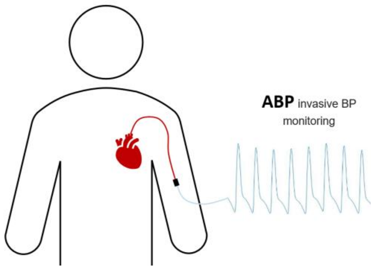
- For continuous monitoring, the invasive arterial catheter method is used, which has potential risks to patients, such as infection and various vascular damage (Figure 1).
- For intermittent monitoring, an occluding arm cuff (sphygmomanometer) is used, and BP is obtained either manually (by auscultation of Korotkoff sounds or palpation) or automatically (by oscillometry) [9]. The Holter blood pressure monitor (HBPM) allows for intermittent measurements (for example, once every fifteen or thirty minutes), which might last up to two days [10].
1.1. Physiological Signals: ECG, PPG, ABP
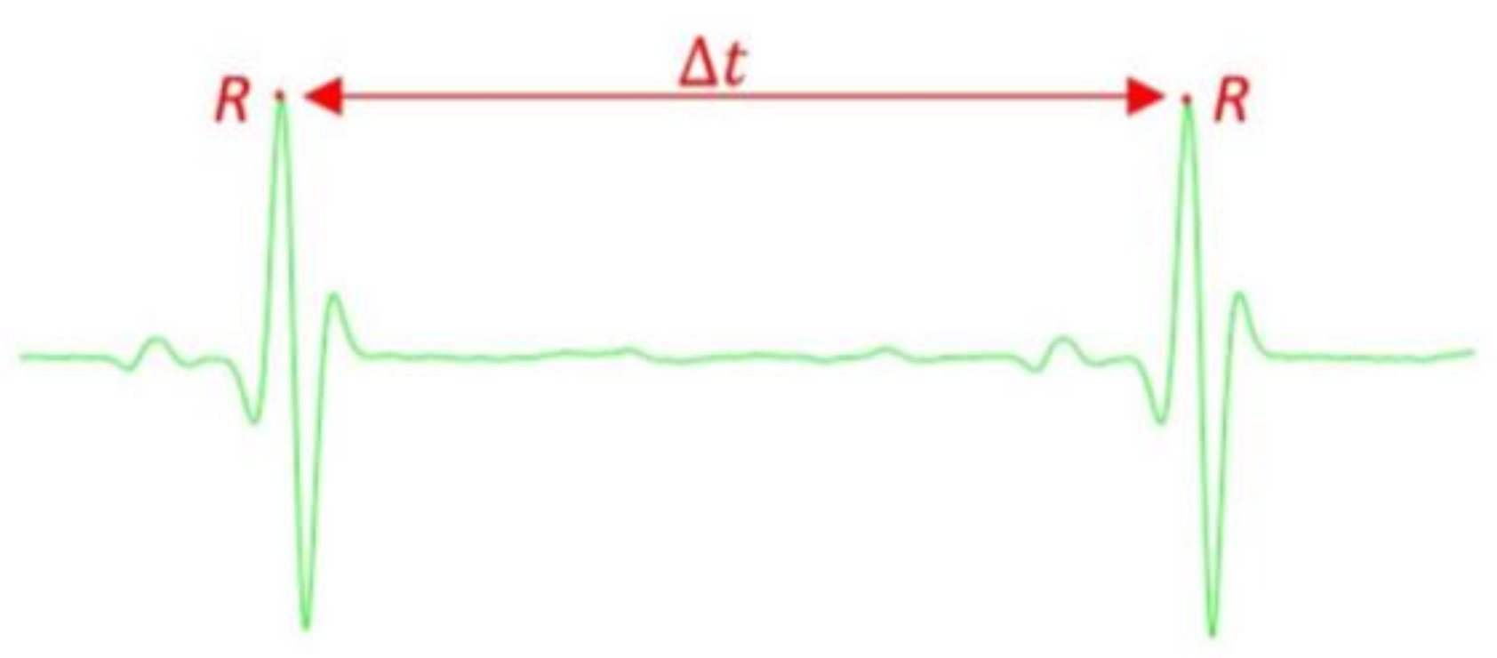
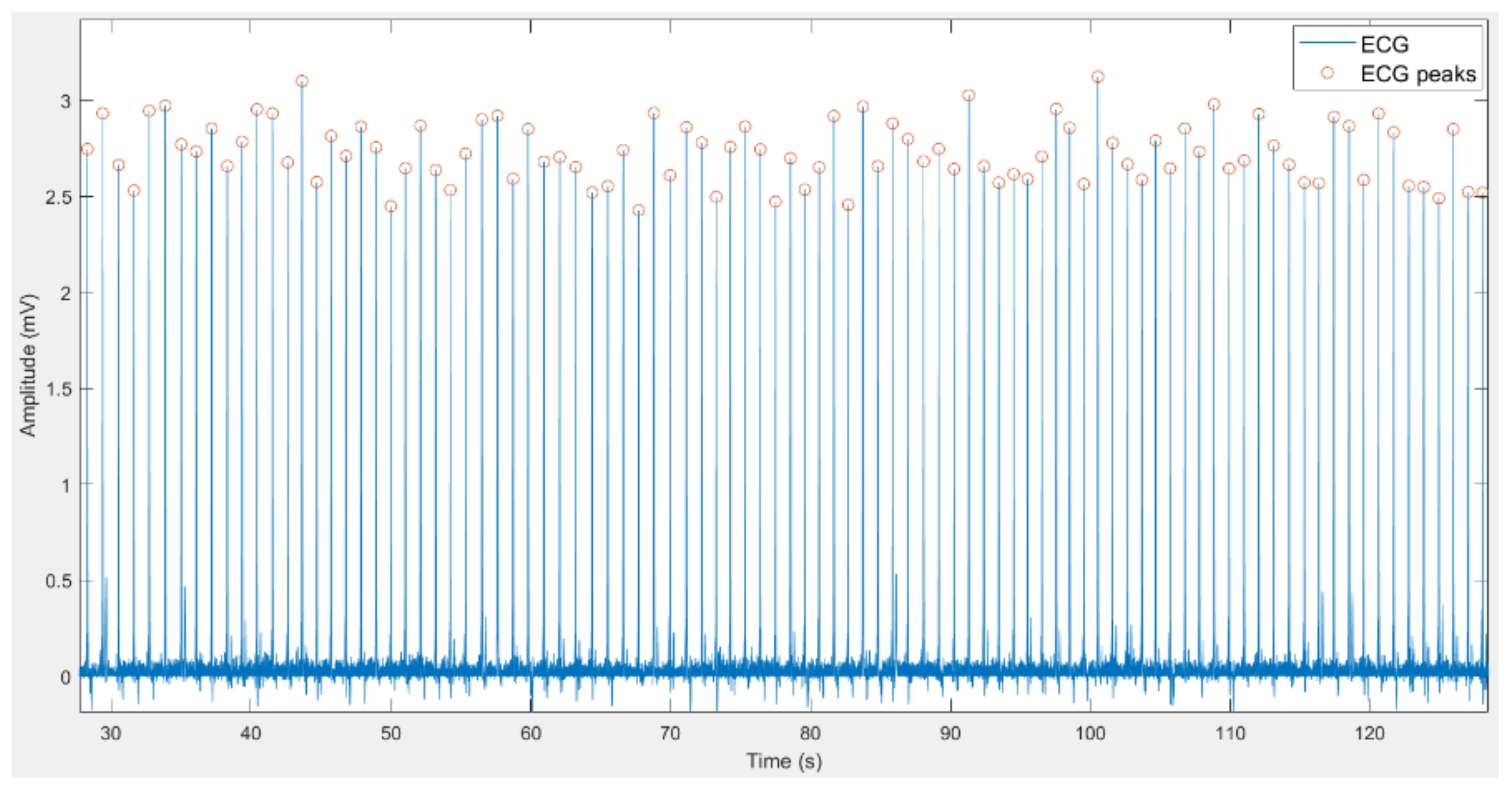
1.1.1. Electrocardiogram
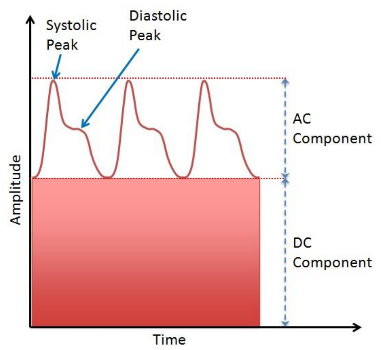
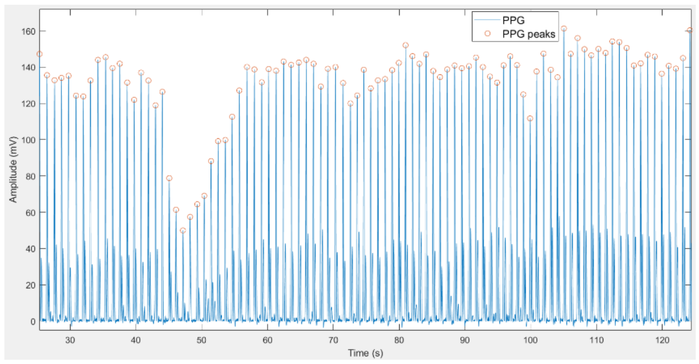
1.1.2. Photoplethysmogram
- The AC component represents blood volume cardiac variation in each heartbeat, and it is attributed to the pulsatile behavior of the heart [28].
- The DC component is highly correlated to central and periphery venous pressure [29]. The average blood volume changes slowly over time, but rapid changes could be caused by several factors, e.g., breathing, presence of a disease, vasomotor activity, sympathetic nervous system activity, and thermoregulation [30].
1.1.3. Arterial Blood Pressure
2. Methods
2.1. Data Collection
2.1.1. MIMIC III Database
- Presence of all ECG, PPG, and ABP signals.
- Presence of peaks or periodicity for more than 5 s.
- About 50 s length for each signal.
- Absence of any peaks (leading to erroneous estimate of HR and PTT features) was noticed for more than 1 s.
- HR or PTT estimated after this process were physically impossible (e.g., DBP reaches 0 mmHg).
- Possible lack of synchronization between the signals.
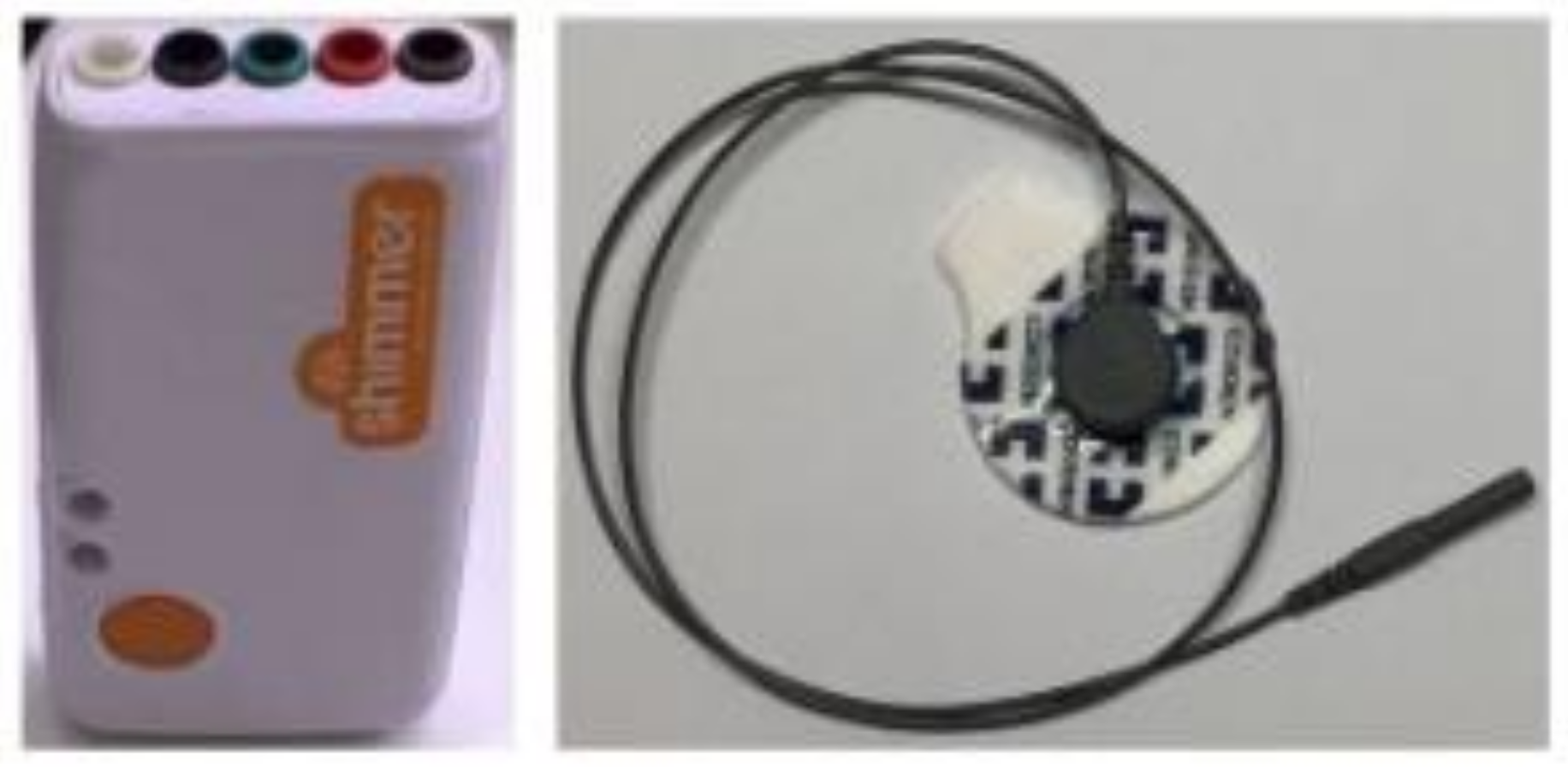
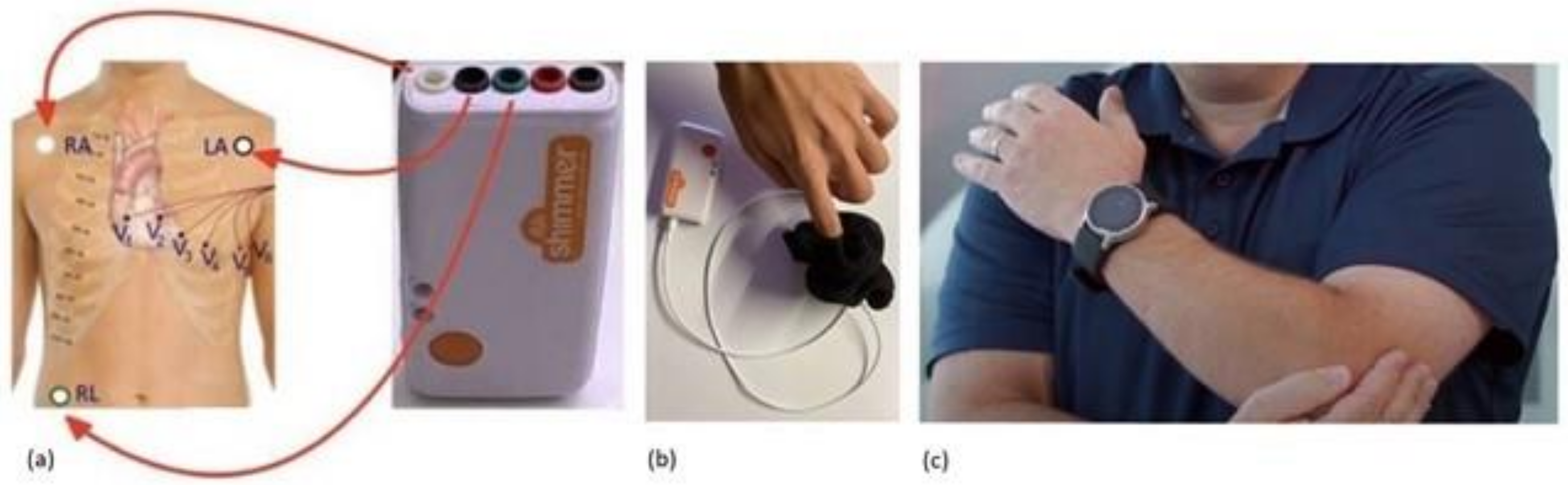
2.1.2. SHIMMER Database
2.2. Data Processing
2.2.1. Filtering of Signals
- fL = 1 Hz
- fH = 10 Hz
- Cutoff frequency = 50 Hz
- Attenuation frequency = 30 Hz
- Band-pass ripple = 0.1 dB
- Stopband attenuation = 15 dB
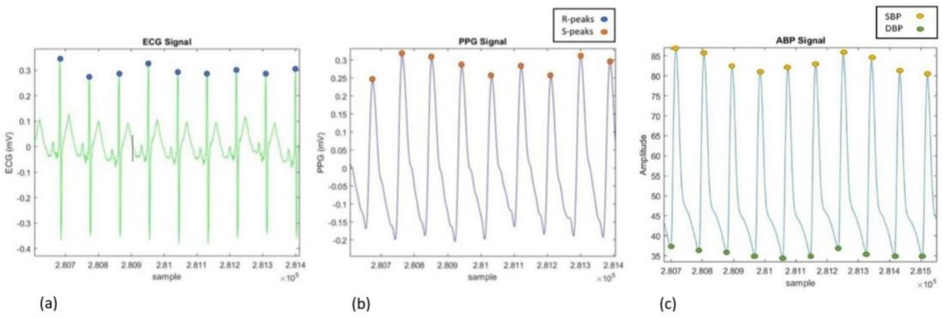
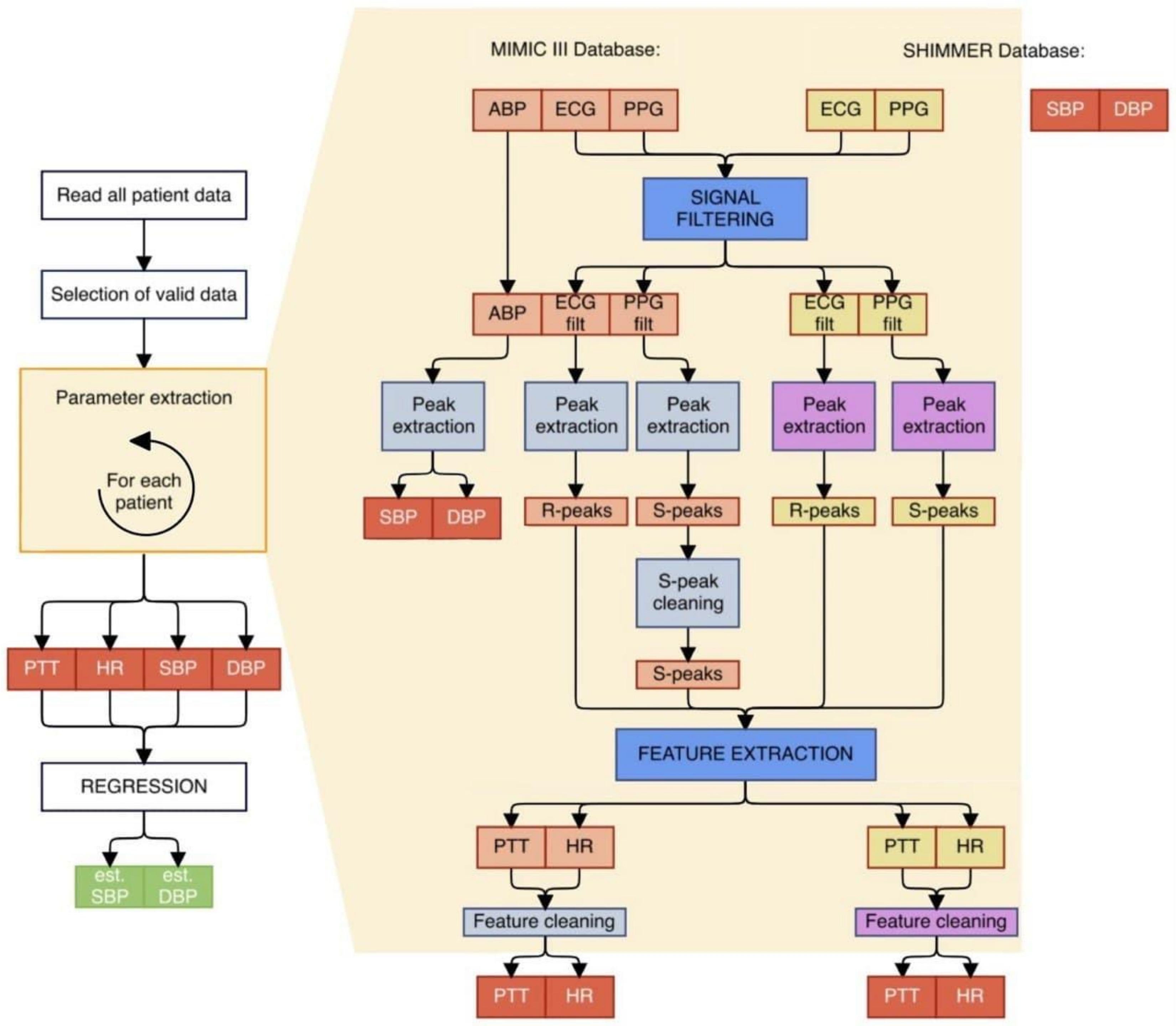
2.2.2. Feature Extraction
Extraction for MIMIC III Database
Extraction for SHIMMER Database
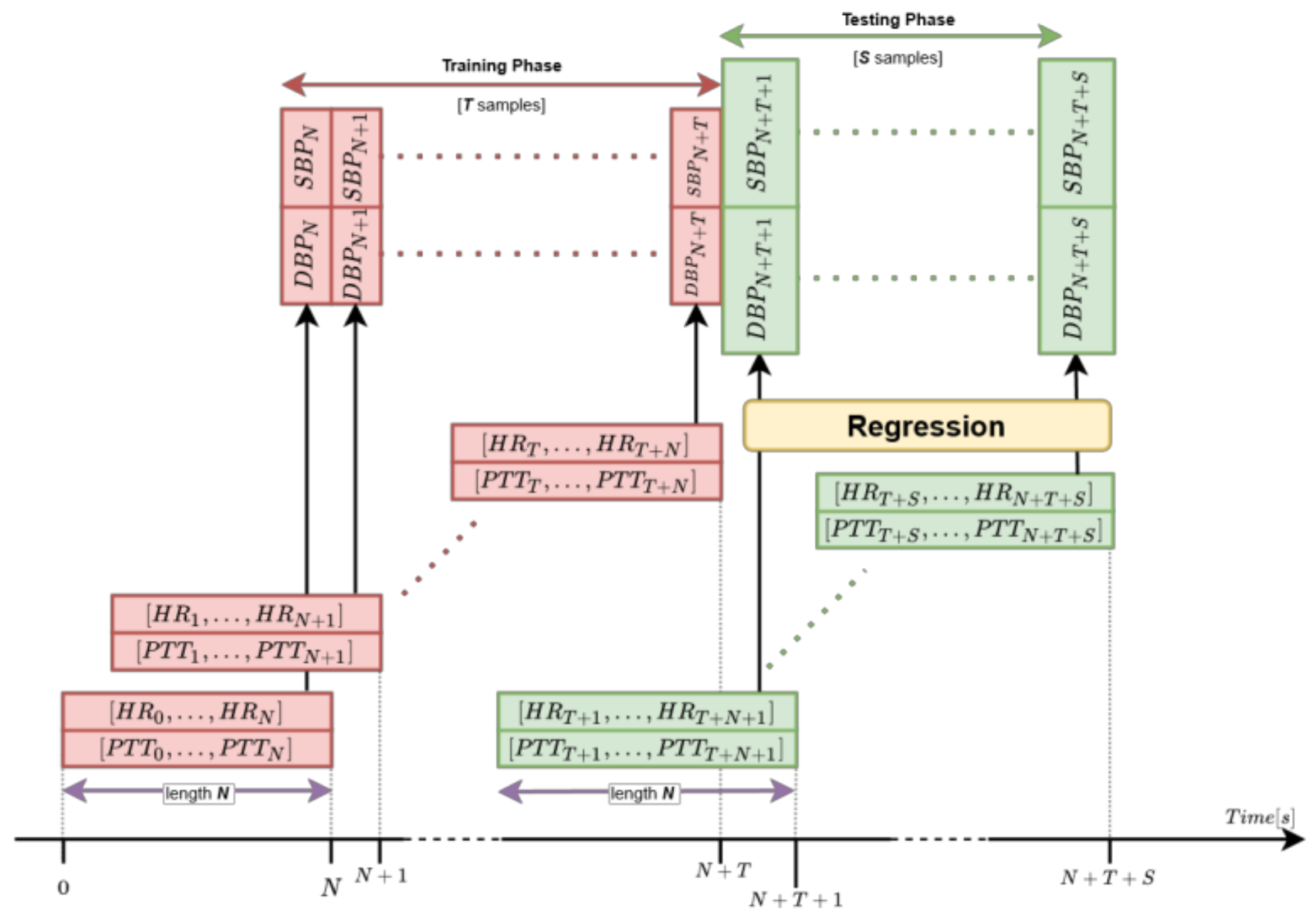
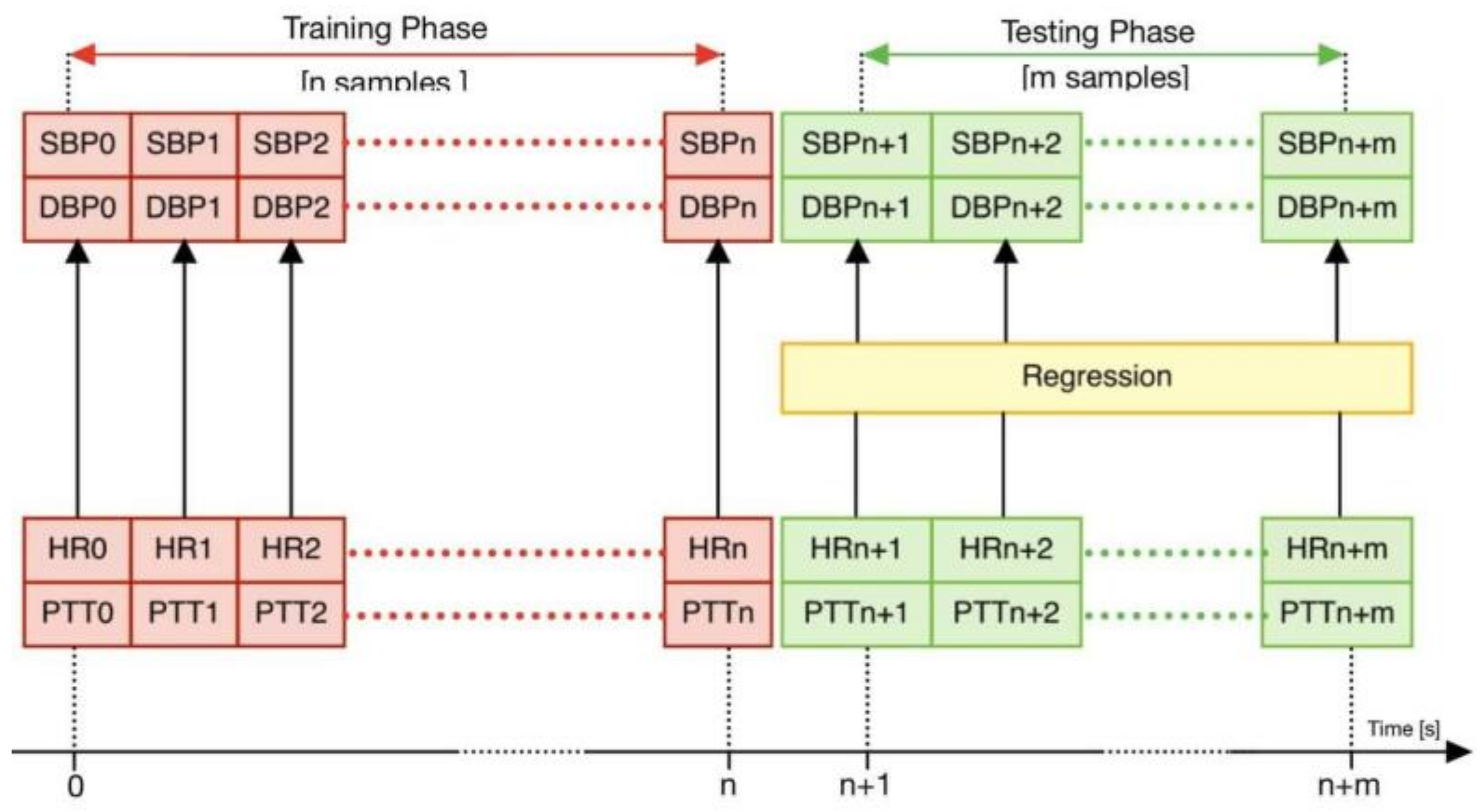
2.2.3. Regression Process
3. Results
3.1. Testing
3.2. Regression Model Selection
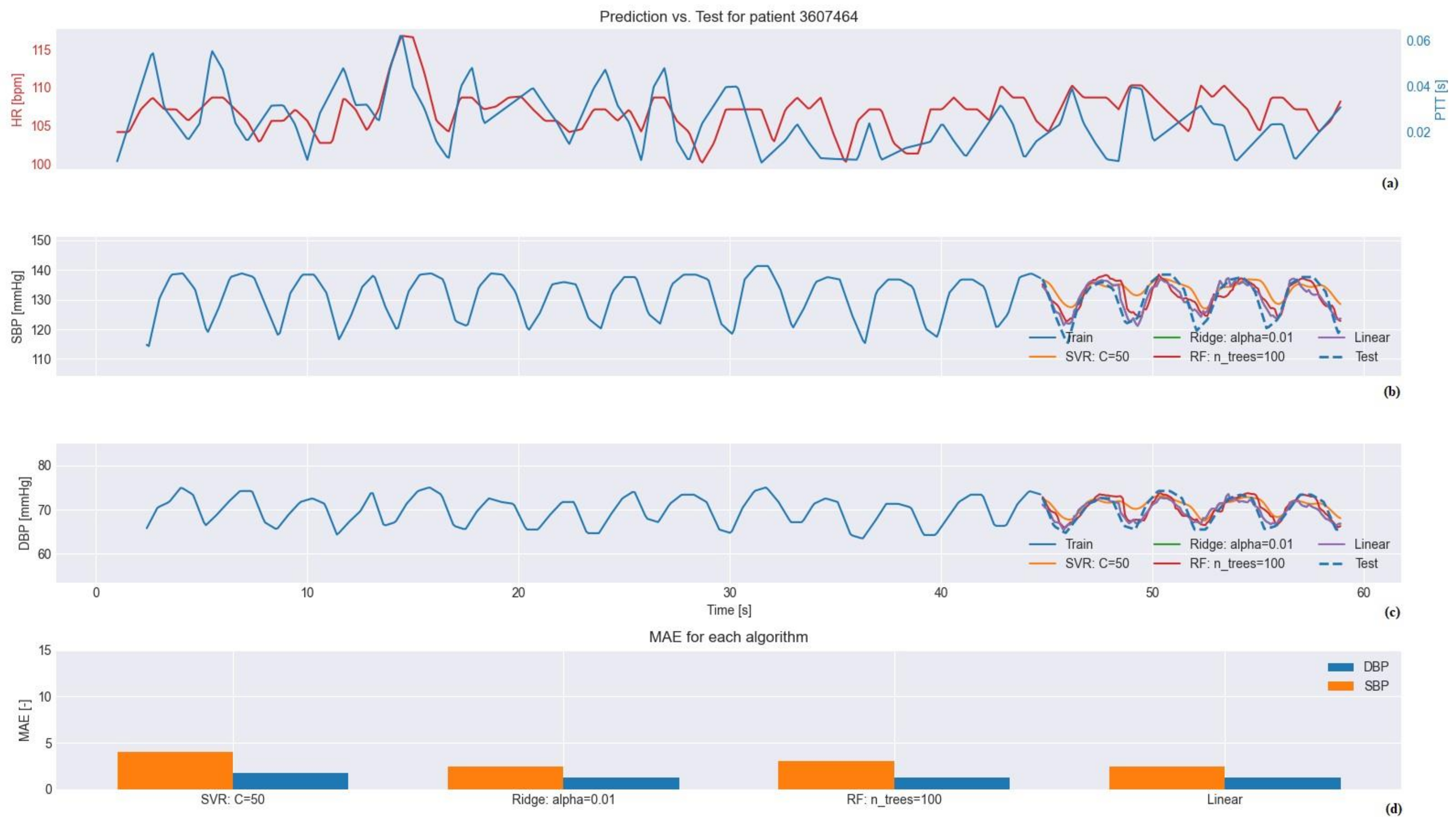
3.2.1. Selection for MIMIC III Database
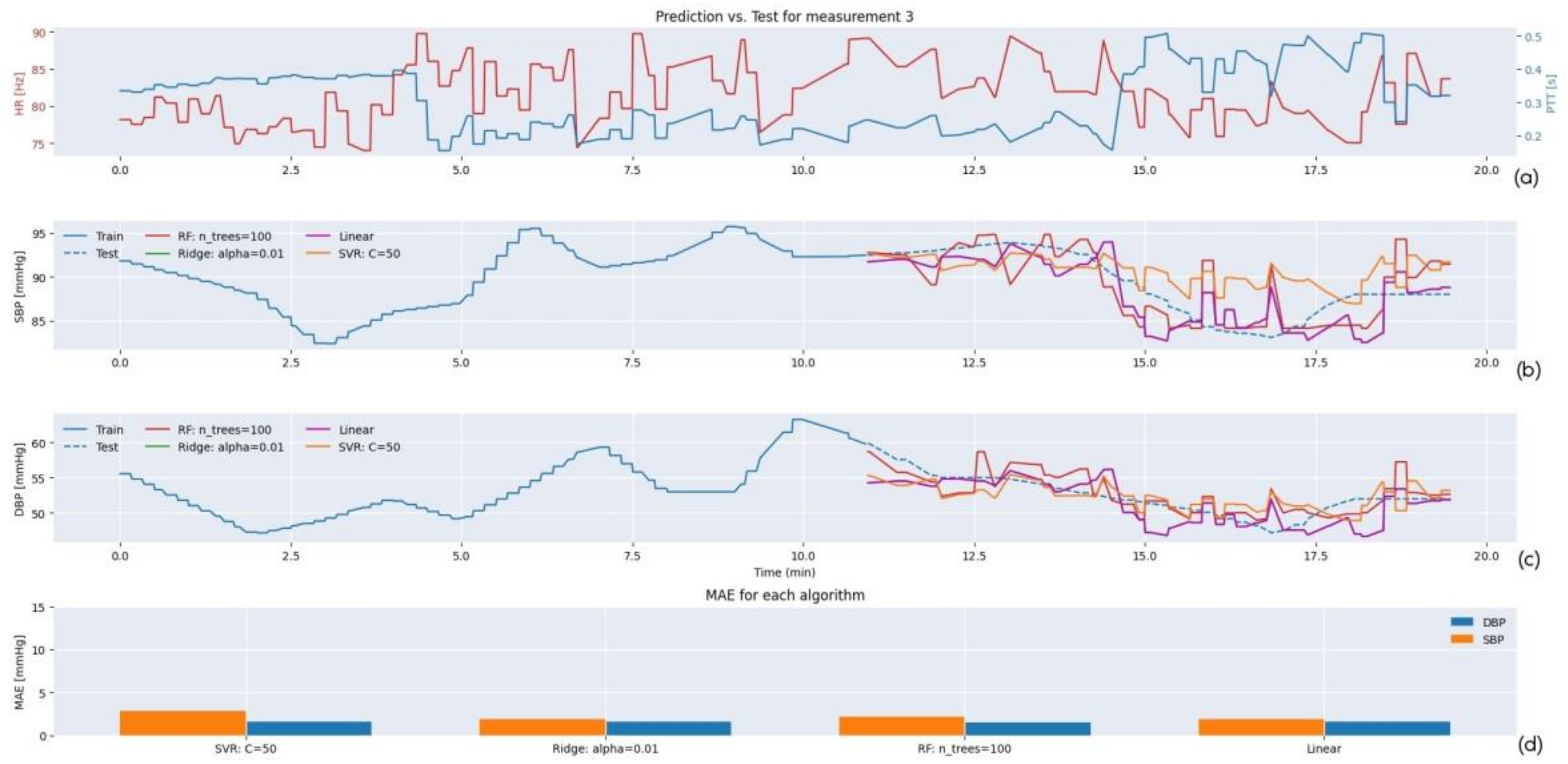
3.2.2. Selection for SHIMMER Database
4. Conclusions
- The innovative way for the removal of outliers (possibly caused by malfunctioning of the hardware and/or the malpositioning of the SHIMMER sensors) using SD for signals from both databases.
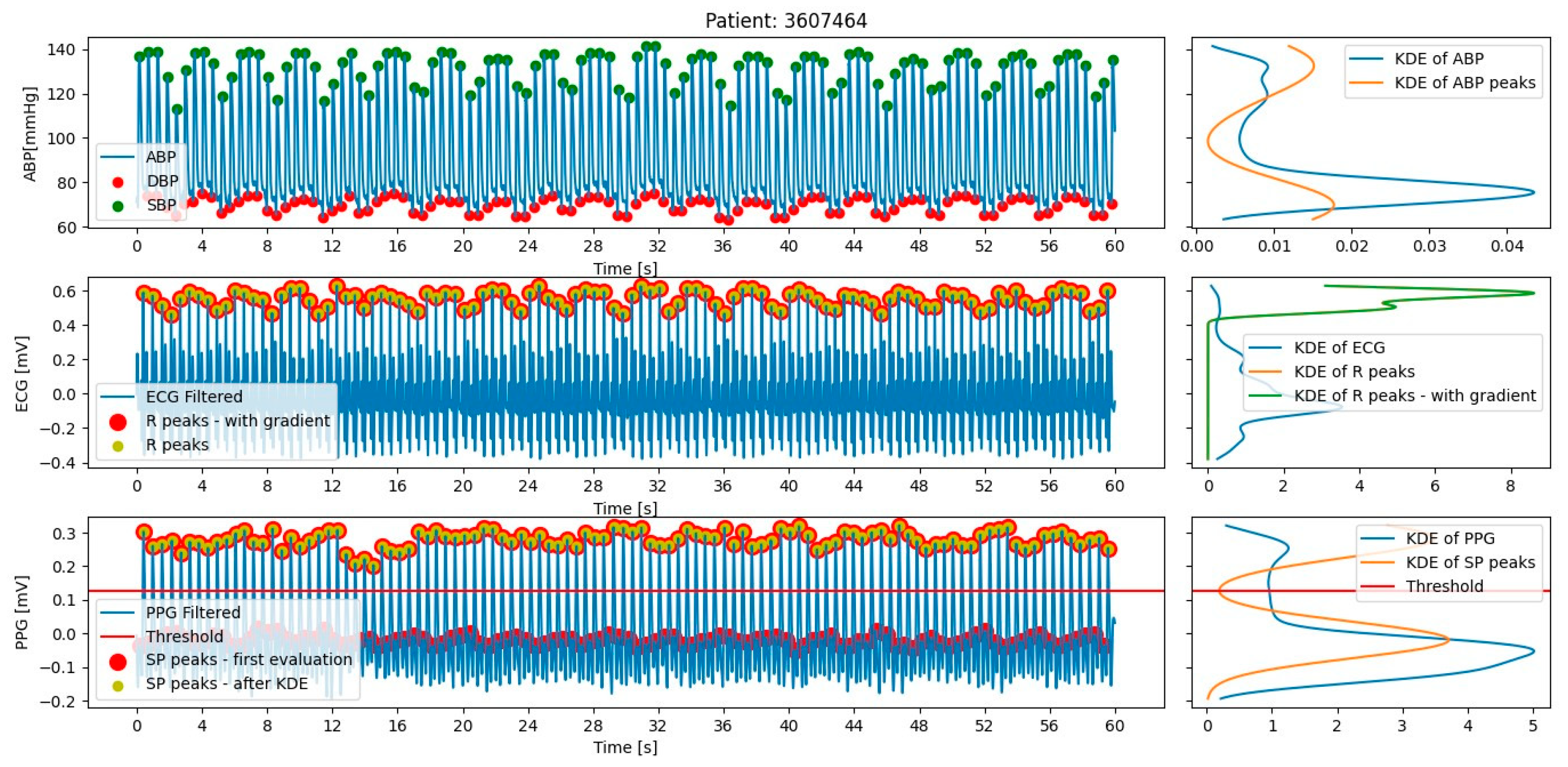
- The efficient and tailored method for the identification of peaks by KDE for signals from the MIMIC III database.
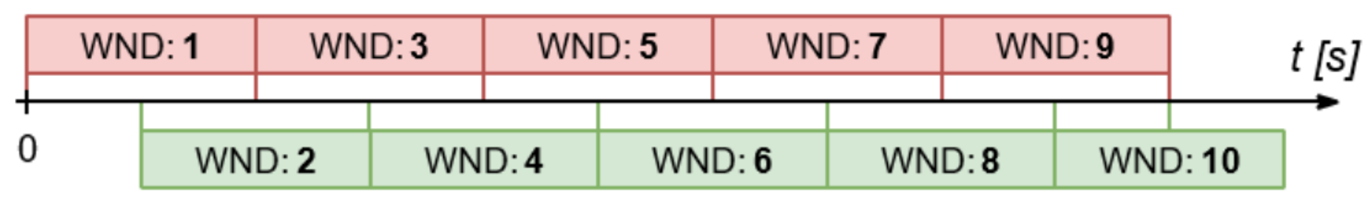
- The use of a sliding window with a time period equal to the period of about two cardiac cycles (T = 1.5 s) for signals from the MIMIC III database.
- The use of ECG and PPG signals acquired from healthy subjects with wearable (SHIMMER) devices.
Author Contributions
Funding
Institutional Review Board Statement
Informed Consent Statement
Data Availability Statement
Acknowledgments
Conflicts of Interest
Abbreviations
| ABP | Arterial blood pressure |
| BP | Blood pressure |
| DBP | Diastolic blood pressure |
| ECG | Electrocardiogram |
| HBPM | Holter blood pressure monitor |
| HR | Heart rate |
| KDE | Kernel density estimation |
| MAE | Mean absolute error |
| PPG | Photoplethysmogram |
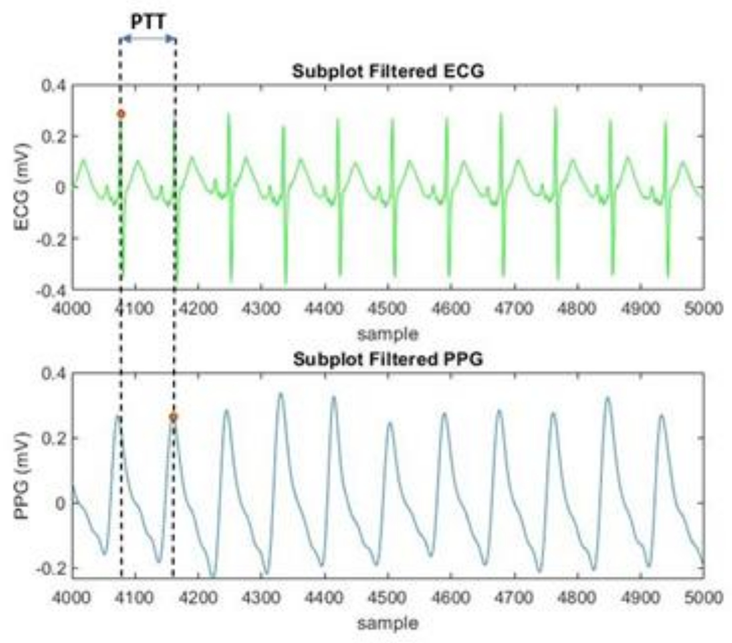
| PTT | Pulse transit time |
| SBP | Systolic blood pressure |
| SD | Standard deviation |
| SVR | Support vector regression |
References
- Arima, H.; Barzi, F.; Chalmers, J. Mortality patterns in hypertension. J. Hypertens. 2011, 29, S3–S7. [Google Scholar] [CrossRef] [PubMed]
- Rahimi, K.; Emdin, C.A.; MacMahon, S. The Epidemiology of Blood Pressure and Its Worldwide Management. Circ. Res. 2015, 116, 925–936. [Google Scholar] [CrossRef] [PubMed] [Green Version]
- Martínez, G.; Howard, N.; Abbott, D.; Lim, K.; Ward, R.; Elgendi, M. Can Photoplethysmography Replace Arterial Blood Pressure in the Assessment of Blood Pressure? J. Clin. Med. 2018, 7, 316. [Google Scholar] [CrossRef] [PubMed] [Green Version]
- Hermida, R.C.; Smolensky, M.H.; Ayala, D.E.; Portaluppi, F. Ambulatory Blood Pressure Monitoring (ABPM) as the reference standard for diagnosis of hypertension and assessment of vascular risk in adults. Chronobiol. Int. 2015, 32, 1329–1342. [Google Scholar] [CrossRef]
- Sun, Z. Aging, arterial stiffness, and hypertension. Hypertension 2015, 65, 252–256. [Google Scholar] [CrossRef] [Green Version]
- Callaghan, F.J.; Geddes, L.A.; Babbs, C.F.; Bourland, J.D. Relationship between pulse-wave velocity and arterial elasticity. Med. Biol. Eng. Comput. 1986, 24, 248–254. [Google Scholar] [CrossRef] [Green Version]
- Pinto, E. Blood pressure and ageing. Postgrad. Med. J. 2007, 83, 109–114. [Google Scholar] [CrossRef]
- Geddes, L.A. Handbook of Blood Pressure Measurement; Springer Science & Business Media: Berlin/Heidelberg, Germany, 1991. [Google Scholar]
- Meidert, A.S.; Saugel, B. Techniques for Non-Invasive Monitoring of Arterial Blood Pressure. Front. Med. 2018, 4, 231. [Google Scholar] [CrossRef]
- Shimbo, D.; Abdalla, M.; Falzon, L.; Townsend, R.R.; Muntner, P. Role of Ambulatory and Home Blood Pressure Monitoring in Clinical Practice: A Narrative Review. Ann. Intern. Med. 2015, 163, 691–700. [Google Scholar] [CrossRef] [Green Version]
- Solà, J.; Delgado-Gonzalo, R. Pulse arrival time techniques. In The Handbook of Cuffless Blood Pressure Monitoring; Delgado-Gonzalo, J.S.R., Ed.; Springer Nature: Berlin/Heidelberg, Germany, 2019; pp. 43–59. [Google Scholar]
- Esmaili, A.; Kachuee, M.; Shabany, M. Nonlinear Cuff-less Blood Pressure Estimation of Healthy Subjects Using Pulse Transit Time and Arrival Time. IEEE Trans. Instrum. Meas. 2017, 66, 3299–3308. [Google Scholar] [CrossRef] [Green Version]
- Moharram, M.; Wilson, L.; Williams, M.; Coffey, S. Beat-to-beat blood pressure measurement using a cuffless device does not accu-rately reflect invasive blood pressure. Int. Cardiol. Hypertens. 2020, 5, 100030. [Google Scholar] [CrossRef] [PubMed]
- Sharma, M.; Barbosa, K.; Ho, V.; Griggs, D.; Ghirmai, T.; Krishnan, S.; Hsiai, T.; Chiao, J.C.; Cao, H. Cuff-Less and Continuous Blood Pressure Monitoring: A Methodological Review. Technologies 2017, 5, 21. [Google Scholar] [CrossRef] [Green Version]
- Mukherjee, R.; Ghosh, S.; Gupta, B.; Chakravarty, T. A literature review on current and proposed technologies of noninvasive blood pressure measurement. Telemed. e-Health 2017, 24, 185–193. [Google Scholar] [CrossRef] [PubMed]
- Ding, X.; Yan, B.P.; Zhang, Y.; Liu, J.; Zhao, N.; Tsang, H.K. Pulse Transit Time Based Continuous Cuffless Blood Pressure Estimation: A new extension and a comprehensive evaluation. Sci. Rep. 2017, 7, 1–11. [Google Scholar] [CrossRef] [PubMed]
- Chen, W.; Kobayashi, T.; Ichikawa, S.; Takeuchi, Y.; Togawa, T. Continuous estimation of systolic blood pressure using the pulse arrival time and intermittent calibration. Med. Biol. Eng. Comput. 2000, 38, 569–574. [Google Scholar] [CrossRef]
- Simjanoska, M.; Gjoreski, M.; Gams, M.; Bogdanova, A.M. Non-Invasive Blood Pressure Estimation from ECG Using Machine Learning Techniques. Sensors 2018, 18, 1160. [Google Scholar] [CrossRef] [PubMed] [Green Version]
- Gesche, H.; Grosskurth, D.; Küchler, G.; Patzak, A. Continuous blood pressure measurement by using the pulse transit time: Comparison to a cuff-based method. Eur. J. Appl. Physiol. 2012, 112, 309–315. [Google Scholar] [CrossRef]
- Wong, M.Y.; Poon, C.C.; Zhang, Y.T. An evaluation of the cuffless blood pressure estimation based on pulse transit time technique: A half year study on normotensive subjects. Cardiovasc. Eng. 2009, 9, 32–38. [Google Scholar] [CrossRef]
- Poon, C.; Zhang, Y. Cuff-less and noninvasive measurements of arterial blood pressure by pulse transit time. In Proceedings of the 2005 IEEE Engineering in Medicine and Biology 27th Annual Conference, Shanghai, China, 17–18 January 2006. [Google Scholar]
- Wang, R.; Jia, W.; Mao, Z.H.; Sclabassi, R.J.; Sun, M. Cuff-Free Blood Pressure Estimation Using Pulse Transit Time and Heart Rate. In Proceedings of the 12th International Conference on Signal Processing (ICSP), Hangzhou, China, 19–23 October 2014. [Google Scholar] [CrossRef] [Green Version]
- Rajni, R.; Inderbir, K. Electrocardiogram Signal Analysis—An Overview. Int. J. Comput. Appl. 2013, 84, 22–25. [Google Scholar] [CrossRef]
- Yu, Q.; Liu, A.; Liu, T.; Mao, Y.; Chen, W.; Liu, H. ECG R-wave peaks marking with simultaneously recorded continuous blood pressure. PLoS ONE 2019, 14, e0214443. [Google Scholar] [CrossRef]
- Kavya, R.; Nayana, N.; Karangale, K.B.; Madhura, H.; Sheela, S.J. Photoplethysmography—A Modern Approach and Applications. In Proceedings of the International Conference for Emerging Technology (INCET), Belgaum, India, 5–7 June 2020; pp. 1–4. [Google Scholar] [CrossRef]
- Ding, X.R.; Zhang, Y.T. Photoplethysmogram intensity ratio: A potential indicator for improving the accuracy of PTT-based cuffless blood pressure estimation. In Proceedings of the 37th Annual International Conference of the IEEE Engineering in Medicine and Biology Society (EMBC), Milan, Italy, 25–29 August 2015. [Google Scholar] [CrossRef]
- NEWS Medical Life Sciences: Photoplethysmography (PPG). Available online: https://www.news-medical.net/health/Photoplethysmography-(PPG).aspx (accessed on 1 October 2020).
- Moraes, J.L.; Rocha, M.X.; Vasconcelos, G.G.; Vasconcelos Filho, J.E.; De Albuquerque VH, C.; Alexandria, A.R. Advances in photopletysmography signal analysis for biomedical applications. Sensors 2018, 18, 1894. [Google Scholar] [CrossRef] [PubMed] [Green Version]
- Lee, C.; Shin, H.S.; Lee, M. Relations between ac-dc components and optical path length in photoplethys-mography. J. Biomedical. Opt. 2011, 16, 077012. [Google Scholar] [CrossRef] [PubMed]
- Allen, J. Photoplethysmography and its application in clinical physiological measurement. Physiol. Meas. 2007, 28, R1. [Google Scholar] [CrossRef] [PubMed] [Green Version]
- Nichols, W.W.; Denardo, S.J.; Wilkinson, I.B.; McEniery, C.M.; Cockcroft, J.; O’Rourke, M.F. Effects of Arterial Stiffness, Pulse Wave Velocity, and Wave Reflections on the Central Aortic Pressure Waveform. J. Clin. Hypertens. 2008, 10, 295–303. [Google Scholar] [CrossRef] [Green Version]
- Muntner, P.; Shimbo, D.; Carey, R.M.; Charleston, J.B.; Gaillard, T.; Misra, S.; Myers, M.G.; Ogedegbe, G.; Schwartz, J.E.; Townsend, R.R.; et al. Measurement of Blood Pressure in Humans: A scientific statement from the American Heart Association. Hypertension 2019, 73, e35–e66. [Google Scholar] [CrossRef]
- Moens, A.I. Die Pulscurve; Brill: Leiden, The Netherlands, 1878. [Google Scholar]
- Proença, J.; Muehlsteff, J.; Aubert, X.; Carvalho, V. Is pulse transit time a good indicator of blood pressure changes during short physical exercise in a young population? Annu. Int. Conf. IEEE Eng. Med. Biol. Soc. 2010, 2010, 598–601. [Google Scholar] [CrossRef]
- Yan, Y.; Zhang, Y. A novel calibration method for non-invasive blood pressure measurement using pulse transit time. In Proceedings of the 4th IEEE/EMBS International Summer School and Symposium on Medical Devices and Biosensors, Cambridge, UK, 19–22 August 2007. [Google Scholar]
- PhysioBank ATM. Available online: https://archive.physionet.org/cgi-bin/atm/atm (accessed on 1 September 2020).
- Shimmer Devices Website. Available online: https://shimmersensing.com/ (accessed on 1 September 2020).
- Omron HeartGuide Website. Available online: https://www.omron-healthcare.co.uk/ (accessed on 1 September 2020).
- Johnson, A.E.; Pollard, T.J.; Shen, L.; Lehman LW, H.; Feng, M.; Ghassemi, M.; Mark, R.G. MIMIC-III, a freely accessible critical care database. Sci. Data 2016, 3, 1–9. Available online: http://www.nature.com/articles/sdata201635 (accessed on 1 September 2020). [CrossRef] [Green Version]
- Mukkamala, R.; Hahn, J.O.; Inan, O.T.; Mestha, L.K.; Kim, C.S.; Töreyin, H.; Kyal, S. Toward Ubiquitous Blood Pressure Monitoring via Pulse Transit Time: Theory and Practice. IEEE Trans. Biomed. Eng. 2015, 62, 1879–1901. [Google Scholar] [CrossRef] [Green Version]
- Burns, A.; Doheny, E.P.; Greene, B.R.; Foran, T.; Leahy, D.; O’Donovan, K.; McGrath, M.J. SHIMMER™: An extensible platform for physiological signal capture. In Proceedings of the 2010 annual international conference of the IEEE engineering in medicine and biology, Buenos Aires, Argentina, 31 August–4 September 2010. [Google Scholar]
- Barlett, M.S. Periodogram analysis and continuous spectra. Biometrika 1950, 37, 1–16. [Google Scholar] [CrossRef]
- Lazazzera, R.; Belhaj, Y.; Carrault, G. A New Wearable Device for Blood Pressure Estimation Using Photoplethysmogram. Sensors 2019, 19, 2557. [Google Scholar] [CrossRef] [Green Version]
- Yadav, U.; Abbas, S.N.; Hatzinakos, D. Evaluation of PPG biometrics for authentication in different states. In Proceedings of the 2018 International Conference on Biometrics (ICB), Gold Coast, QLD, Australia, 20–23 February 2018. [Google Scholar]
- Ridge Regression NCSS Statistical Software NCSS.com335-1© NCSS, LLC. All Rights Reserved Chapter 335. Available online: https://ncss-wpengine.netdna-ssl.com/wp-content/themes/ncss/pdf/Procedures/NCSS/Ridge_Regression.pdf (accessed on 1 July 2020).
- Stergiou, G.S.; Alpert, B.; Mieke, S.; Asmar, R.; Atkins, N.; Eckert, S.; Frick, G.; Friedman, B.; Graßl, T.; Ichikawa, T.; et al. A universal standard for the validation of blood pressure measuring devices: Association for the Advancement of Medical Instrumentation/European Society of Hypertension/International Organization for Standardization (AAMI/ESH/ISO) Collaboration Statement. J. Hypertens. 2018, 36, 472–478. [Google Scholar] [CrossRef] [PubMed]
- Vernier: What Are Mean Squared Error and Root Mean Squared Error? Available online: https://www.vernier.com/til/1014 (accessed on 1 November 2020).
- Wang, W.; Lu, Y. Analysis of the Mean Absolute Error (MAE) and the Root Mean Square Error (RMSE) in Assessing Rounding Model. IOP Conf. Ser. Mater. Sci. Eng. 2018, 324, 012049. [Google Scholar] [CrossRef]
- Guidelines on Medical Devices. European Commission Dg Internal Market, Industry, Entrepreneurship and SMEs Consumer, Environmental and Health Technologies Health technology and Cosmetics (June 2016). Available online: https://ec.europa.eu/docsroom/documents/17522/attachments/1/translations/en/renditions/native (accessed on 1 January 2022).
- Dorugade, A.V.; Kashid, D.N. Alternative method for choosing ridge parameter for regression. Appl. Math. Sci. 2010, 4, 447–456. [Google Scholar]
- SINTEC. Available online: https://www.sintec-project.eu/ (accessed on 27 February 2022).


| AVERAGE MAE (mmHg) ± AVERAGE SD (mmHg) | ||||||||
|---|---|---|---|---|---|---|---|---|
| Linear Regressor | Random Forest Regressor | Ridge Regressor | SVR | |||||
| SBP | DBP | SBP | DBP | SBP | DBP | SBP | DBP | |
| MIMIC III database | 3.16 ± 1.96 | 2.01 ± 1.43 | 3.16 ± 1.96 | 1.95 ± 1.37 | 3.20 ± 2.20 | 2.01 ± 1.42 | 3.20 ± 2.38 | 1.83 ± 1.33 |
| SHIMMER database | 1.76 ± 1.67 | 1.76 ± 1.72 | 2.98 ± 3.26 | 2.50 ± 2.53 | 1.76 ± 1.67 | 1.76 ± 1.72 | 2.62 ± 0.87 | 2.47 ± 0.84 |
| Average MAE (mmHg) | ||
|---|---|---|
| Regression Model | DBP | SBP |
| Ridge Regressor | 3.23 ± 0.80 | 4.03 ± 0.87 |
| Linear Regressor | 3.57 ± 1.47 | 4.07 ± 0.92 |
| SVR | 2.15 ± 0.09 | 3.12 ± 0.09 |
| Random Forest Regressor | 2.23 ± 0.13 | 3.14 ± 0.23 |
| DBP’s Average MAE (mmHg) | SBP’s Average MAE (mmHg) | Number of Subjects | |
|---|---|---|---|
| Random Forest Regressor | 1.95 ± 1.37 | 3.16 ± 1.96 | 90 |
| AAMI guidelines | ≤5 | ≤5 | ≥85 |
| DBP’s Average MAE (mmHg) | SBP’s Average MAE (mmHg) | Number of Measurements | |
|---|---|---|---|
| Linear Regressor | 1.76 ± 1.72 | 1.76 ± 1.67 | 50 |
| AAMI guidelines + OMRON HeartGuide accuracy (±3 mmHg) | ≤2 | ≤2 | ≥35 |
Publisher’s Note: MDPI stays neutral with regard to jurisdictional claims in published maps and institutional affiliations. |
© 2022 by the authors. Licensee MDPI, Basel, Switzerland. This article is an open access article distributed under the terms and conditions of the Creative Commons Attribution (CC BY) license (https://creativecommons.org/licenses/by/4.0/).
Share and Cite
Figini, V.; Galici, S.; Russo, D.; Centonze, I.; Visintin, M.; Pagana, G. Improving Cuff-Less Continuous Blood Pressure Estimation with Linear Regression Analysis. Electronics 2022, 11, 1442. https://doi.org/10.3390/electronics11091442
Figini V, Galici S, Russo D, Centonze I, Visintin M, Pagana G. Improving Cuff-Less Continuous Blood Pressure Estimation with Linear Regression Analysis. Electronics. 2022; 11(9):1442. https://doi.org/10.3390/electronics11091442
Chicago/Turabian StyleFigini, Valeria, Sofia Galici, Daniele Russo, Ilenia Centonze, Monica Visintin, and Guido Pagana. 2022. "Improving Cuff-Less Continuous Blood Pressure Estimation with Linear Regression Analysis" Electronics 11, no. 9: 1442. https://doi.org/10.3390/electronics11091442
APA StyleFigini, V., Galici, S., Russo, D., Centonze, I., Visintin, M., & Pagana, G. (2022). Improving Cuff-Less Continuous Blood Pressure Estimation with Linear Regression Analysis. Electronics, 11(9), 1442. https://doi.org/10.3390/electronics11091442