Abstract
Arterial blood pressure is not only an important index that must be measured in routine physical examination but also a key monitoring parameter of the cardiovascular system in cardiac surgery, drug testing, and intensive care. To improve the measurement accuracy of continuous blood pressure, this paper uses photoplethysmography (PPG) signals to estimate diastolic blood pressure and systolic blood pressure based on ensemble empirical mode decomposition (EEMD) and temporal convolutional network (TCN). In this method, the clean PPG signal is decomposed by EEMD to obtain n-order intrinsic mode functions (IMF), and then the IMF and the original PPG are input into the constructed TCN neural network model, and the results are output. The results show that TCN has better performance than CNN, CNN-LSTM, and CNN-GRU. Using the data added with IMF, the results of the above neural network model are better than those of the model with only PPG as input, in which the systolic blood pressure (SBP) and diastolic blood pressure (DBP) results of EEMD-TCN are −1.55 ± 9.92 mmHg and 0.41 ± 4.86 mmHg. According to the estimation results, DBP meets the requirements of the AAMI standard, BHS evaluates it as Grade A, SD of SBP is close to the standard AAMI, and BHS evaluates it as Grade B.
1. Introduction
Globally, hypertension and cardiovascular diseases have been affecting the healthy life of human beings, causing millions of deaths every year and increasing the risk of other diseases [1]. Due to the recent epidemic situation, the cardiovascular status of COVID-19-infected people has attracted people’s attention. Evidence shows that no matter how severe the symptoms of patients in COVID-19 are, more than ordinary people will suffer from cardiovascular problems, and those who recover from COVID-19 may have long-term cardiovascular consequences [2]. Therefore, arterial blood pressure is one of the foremost imperative parameters to characterize the health of the cardiovascular system, and a real-time, dynamic, continuous, and accurate long- and short-range monitoring method is more important [3].
Sleeveless continuous blood pressure measurement belongs to an indirect method of measuring human blood pressure, which has no harm to the human body and is more suitable for being widely used in daily life. At present, the concept of non-contact measurement is getting more and more popular. Continuous monitoring of blood pressure can also provide abundant waveform information, which has important scientific research and clinical value for understanding the influence of external and internal factors on blood pressure and evaluating vascular parameters [4].
The waveform amplitude and shape of PPG contain much important physiological information of the heart and cardiovascular system [5]. A large number of studies have shown a close relationship between blood pressure and PPG, which has led to non-invasive continuous blood pressure estimation methods based on PPG [6,7,8,9,10], including pulse transmission time (PTT) and the method based on the characteristic parameters of the PPG waveform. PTT is ordinarily characterized as the time required for the pulse beat to proliferate from the heart to the fringe of the body. In most cases, PTT can be acquired by one ECG sensor and one PPG sensor or two PPG sensors [11,12]. The PPG waveform parameter method is mainly based on PPG signal waveform and personal information features and uses a machine learning method to establish blood pressure model. This method involves manual extraction and selection of PPG waveform features. After feature engineering, the machine learning method is used to model [13,14,15]. However, whether it is a continuous blood pressure prediction method based on PTT or PPG waveform parameters, the shape of the PPG signal will not only change with aging and some diseases but also the artificially selected feature has great individual differences. This usually leads to poor generalization performance of the model, and it is often necessary to model and calibrate the model individually for individuals. In addition, because the physiological parameters of the human body will change with time, the calibrated model can only keep its accuracy in a short time, so it needs to be calibrated regularly [16,17].
Compared with conventional machine learning, the deep learning method can learn the abstract and complex features of the signal and can fully mine the useful information contained in the signal, which is very suitable for constructing a complex nonlinear model of the blood pressure estimation model [18,19]. In recent years, models using convolution neural networks (CNN), recurrent neural networks LSTM and GRU, and hybrid neural networks CNN-LSTM and CNN-GRU have been applied to the continuous measurement of blood pressure and accomplished great results [20,21,22,23,24,25]. However, traditional CNN has not been able to combine PPG information in the past. Although RNN has great advantages in dealing with time series problems, the RNN model parameters are complex, and the forward transfer of the next time step can only be carried out after the end of the forward transfer of the previous time step, so the model training not only takes a large amount of time but also consumes a large amount of memory [26]. Recently, a special CNN-Temporal convolutional network (TCN) is compared with many RNN structures, and it is found that TCN can reach or even surpass the RNN model in many tasks [27,28,29,30]. Because of the combination of the parallel feature processing of convolutional neural network (CNN) and the time series modeling ability of recurrent neural network (RNN), the features of input signals can be extracted comprehensively.
Therefore, in this paper, we utilize the TCN model to predict SBP and DBP values from PPG signals. In much of the literature, to predict BP better, the original PPG signal and its first derivative and second derivative signals were used as the input of the model and the performance was improved [31,32,33]. Inspired by this idea, we take the modal components after the PPG signal EEMD as the input of the model so that the model can extract more features and improve the accuracy of the model.
The content of this paper can be summarized as follows:
- Only PPG signals are used to predict blood pressure, and a single PPG signal is easier to obtain, and the PPG is segmented with overlapping periods.
- TCN was used as a non-invasive model for continuous blood pressure estimation.
- EEMD is used to expand the input of the model so that the model can extract more features containing PPG information.
The second part of this paper introduces the related work. The third part introduces the related theories and the proposed methods. The fourth part introduces the experimental results. Finally, the fifth part summarizes this paper.
2. Related Work
The blood pressure measurement method based on the PPG signal can be divided into two categories according to whether the features need to be extracted manually or not. One is to extract features manually in advance and then establish a regression algorithm to predict SBP and DBP. Among these methods, the PPT method and PPG parameter method have been widely studied in recent years. Moreover, the rapid development of machine learning provides a new idea for the research of continuous blood pressure monitoring. Viunytskyi et al. believe that the blood pressure measurement method based on the machine learning algorithm is more flexible and can reduce the error of blood pressure monitoring results [34]. Montemoreno et al. have done some research on the use of machine learning technology in blood pressure estimation. They have applied 14 methods, including linear regression, neural network, SVM, random forest, and the final result meets the B standard of BHS [35]. Khalid et al. extracted five different features from a PPG signal segment and trained and tested them by using multiple linear regression, support vector machine (SVM), and regression tree. In general, tests suggest that the blood pressure monitoring algorithm based on the regression tree has the highest precision [36]. Attarpour et al. proposed a monitoring method of SBP and DBP based on wrist and fingertip pulse signals and established a two-layer artificial neural network to monitor SBP and DBP through PWV and PTT features [9]. Hu et al. applied an ensemble machine-learning algorithm to estimate SBP and DBP [37].
The other method uses deep-learning-based technology to end-to-end with PPG signal segment as model input and corresponding SBP and DBP as labels. The deep neural network can automatically extract the fundamental features without any complex feature engineering [38]. Along with the development of computing power, many researchers have begun to establish different continuous blood pressure monitoring models based on deep neural networks. Baek et al. took the time domain and frequency domain forms of PPG signal as input, and successfully estimated SBP and DBP values using a single CNN architecture [39]. El-Hajj and PA Kyriacou used bidirectional long- and short-term memory, bidirectional gated cycle unit, and attention mechanism to estimate SBP and DBP with PPG signal pairs [40]. Wang et al. used a mixed neural network model of CNN and GRU to estimate SBP and DBP [41]. Esmaelpoor et al. proposed a multilevel model based on CNN-LSTM, which combined the dynamic relationship between SBP and DBP to improve the accuracy [16].
TCN has accomplished great results in time series forecasting. Zhao et al. proposed a deep learning framework based on the TCN model for short-term city-wide traffic forecasting, and the experimental results show that TCN achieves state-of-the-art performance in short-term traffic flow forecasting [42]. Song et al. proposed a TCN-based heat load forecasting algorithm that has performance advantages [43]. The combination of EEMD and deep neural networks is applied in many fields, such as Lan et al. In the field of weather prediction, EEMD is utilized to decompose the initial data into subsequences with different frequencies [44]. These subsequences are used as inputs of the SOM-BP network. Chen et al. proposed a short-term wind speed forecast system based on the EEMD-GA-LSTM strategy [45]. Therefore, it is worth trying to use TCN combined with EEMD for continuous blood pressure estimation.
3. Methods
3.1. Empirical Mode Decomposition
Empirical Mode Decomposition (EMD) is a multi-scale signal decomposition method appropriate for non-stationary and nonlinear signals. It can adaptively decompose a signal into the sum of several intrinsic mode functions (IMF); each IMF has a unique frequency component [46]. EMD is decomposed based on the data itself, so it is suitable for arbitrary data. However, there are some problems and shortcomings in this method, mainly that the intrinsic modal function gotten by EMD decomposition has the phenomenon of modal aliasing.
Huang et al. studied the EMD decomposition of white noise [47] and found that EMD decomposition is similar to binary filter, and the energy of white noise is uniformly distributed in its spectrum, so an improved EMD method based on noise-aided analysis, namely EEMD, was proposed. By adding different white noises with the same amplitude each time, the extreme point characteristics of the signal are changed, and then the corresponding IMF obtained by EMD many times is averaged to offset the added white noises, thus effectively suppressing the occurrence of modal aliasing. EEMD decomposition steps are as follows.
Step 1: Set the average total number m;
Step 2: A white noise with a standard normal distribution is added to the original signal to generate a new signal: . Where represents the white noise sequence added for the h time;
Step 3: The signal added with white noise is decomposed by EMD to obtain each IMF component;
Step 4: Repeated EMD decomposition for each group of signals with white noise to obtain m groups of IMF components and m groups of residual Res;
Step 5: Average the IMF population obtained each time as the final result, that is, the J-th modal component = .
The original signal can be expressed as:
In the above decomposition process, because the added white noise has the random characteristics that the mean value is 0 and the variance is equal, the overall mean value of all EMD decomposition is taken as the ultimate decomposition result of the EEMD deterioration IMF component, which disposes of the impact of white noise.
3.2. Temporal Convolutional Network
The temporal convolutional network is a new type of time series forecasting algorithm. The TCN architecture includes dilated causal convolution and residual modules [48]. Compared with LSTM and GRU, TCN has the advantages of low memory occupation, stable gradient, good parallelism, and flexible receptive field.
3.2.1. Causal Dilation Convolution
Causal convolution is a strict time constraint model, for the value of the moment on a layer of t only depends on the next layer of t moment and its previous value. TCN uses causal convolution to enable the output of the current time to mine the information of a period before that time. Basic causal convolution still has the issue of the conventional convolutional neural network, i.e., the modeling length of time is constrained by the size of the convolution kernel. On the off chance that one might need to catch longer dependencies, it would be preferable to stack numerous layers linearly. To unravel this issue, researchers put forward the dilation convolution. The dilation convolution increments the receptive field of the convolution kernel while keeping the number of parameters unaltered, and at the same time, it can guarantee that the size of the output feature map remains unchanged.
We illustrate the structure of causal dilated convolutions with an example, as shown in Figure 1, which depicts dilated causal convolutions with dilation coefficients d of 1, 2, and 4 and convolution kernel k of size 2. The input sequence is and the result of each layer at time t = 8 depends on the value before time t = 8 of the previous layer. Each layer extracts the information of the previous layer, all in the form of interval sampling. The layer-by-layer expansion coefficient increases exponentially by 2, and finally, can extract the information of the sequence. TCN can obtain a large receptive field with fewer layers. In theory, causal dilated convolutions can accept data at any time step as input.
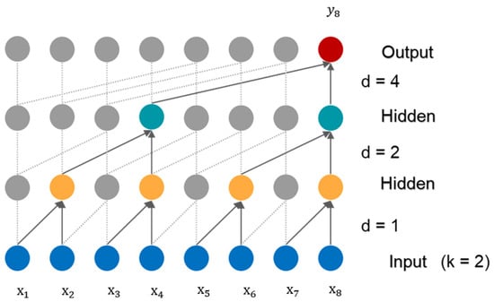
Figure 1.
Causal dilation convolution structure.
3.2.2. Residual Connections
In general, the expressive ability of neural networks gradually increases with the increase of network depth, but the increase of network structure depth may lead to a series of problems such as gradient disappearance and gradient explosion. To further deepen the network depth and improve the ability of the model to learn time-series information, TCN uses a residual module instead of a convolution layer [49]. One residual module consists of two layers of causal dilation convolution layer and nonlinear transformation layer, and regularization technology is used to reduce the risk of over-fitting.
Dropout means that in the process of neuron propagation, the activation value of a neuron will stop working with a certain probability, thus enhancing the generalization of the model; Relu is used as the activation function of the neural network; WeightNorm means normalization of weight value; DilatedCausalConv represents the dilation convolution layer. In some cases, the input and output dimensions are different, so one can also add 1*1 convolution to reduce the dimension of the input, so that the input and output dimensions are the same and can be added together.
Figure 2 shows the overall structure of TCN, which consists of a stack of TCN residual modules and a fully connected layer. The field of view of TCN depends on the network depth n, filter size k, and expansion factor d. The TCN residual module tackles the issue of network depth development, so TCN can make the model have better generalization ability by stacking residual modules.
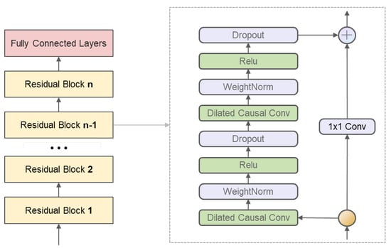
Figure 2.
Temporal convolutional network model structure and residual block structure.
3.3. Proposed BP Estimation Method of EEMD-TCN
The method proposed in this study is based on the frequency decomposition algorithm EEMD and TCN model. Figure 3 shows the method proposed in this paper. First, we decompose the first PPG signal segment into n IMF by EEMD, construct a potential feature set, and then input each group of subsequences and the original PPG signal segment into the TCN prediction model as channels, so that the model can extract more PPG information. The feature set constructed in theory is dynamic, and we can determine which IMF and original PPG are selected to constitute the feature set through experiments, to minimize the error of the model.
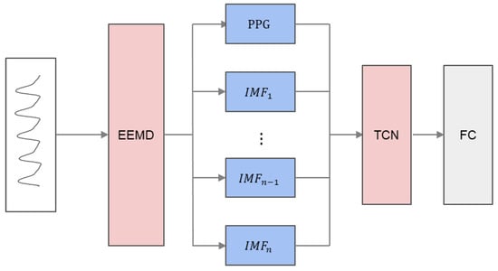
Figure 3.
Structure diagram of EEMD-TCN prediction model.
4. Results
4.1. Dataset
In this paper, we use the blood pressure data set in the machine learning repository. This is the pre-processed clean data from MIMIC-II released by Kachuee et al. [50]. The data set includes PPG, arterial blood pressure (ABP), and ECG signals recorded from fingertips, which were sampled at a frequency of 125 Hz. The MIMIC data set provides subjects of different age groups and genders from hospital ICU, and their blood pressure ranges may be different. We randomly selected 150 samples longer than 8 min, extricated SBP and DBP from invasive blood pressure waveform, and utilized them as target values within the estimation handle. In addition, we removed the sequences of abnormal SBP and DBP values (SBP ≥ 180, DBP ≥ 130, SBP ≤ 80, DBP ≤ 60).
To obtain the SBP and DBP values in invasive continuous blood pressure and the corresponding PPG signals, it is necessary to detect the peaks and valleys of ABP and PPG to segment the signals. There are many ways of signal segmentation, and the conventional segmentation method is fixed-length segmentation or one-to-one segmentation according to the period. However, due to the particularity of signals in MIMIC, there may be a time delay between signals, and the one-to-one segmentation method will lead to the wrong matching between PPG and ABP, which will lead to larger errors. The long segmentation method is easy to operate, but it is easy to destroy the periodic characteristics of the signal. Therefore, this paper adopts a multi-period sliding segmentation method, that is, each segment of the segmented signal contains multiple periods, and some periods overlap between segments. Here, the number of periods of each signal segment is nine, and there are seven periods of overlap between segments. We obtained 11,226 segments, then we scrambled the data, using 80% of the data as the training set and the rest as the test set. In the subsequent experiments, the TCN model accepts the input of signal segments with different lengths, while other deep neural network models need to make each segment equal in length. The feasible ways include zero complements and resampling. In this selection, through resampling, each segment of PPG and ECG is 625 points. The final histogram of blood pressure data distribution is shown in Figure 4. Table 1 shows the statistics of the final data set.
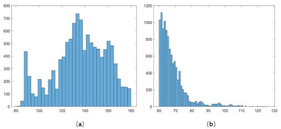
Figure 4.
Histogram of blood pressure distribution: (a) is the data distribution of SBP; (b) is the data distribution of DBP.

Table 1.
Statistics of SBP and DBP in data set.
4.2. Prediction Results of the Original PPG as Input
In this paper, the standard deviation (SD), mean absolute error (MAE) and mean error (ME) on the test set are used as evaluation indexes to verify the performance of the model.
Because the length of each piece of PPG data is less than 1000 when SBP is used as the label, we use TCN of the four-layer network, the convolution kernel size is five, and the dilation rate increases exponentially with the number of layers, which is one, two, four, and eight, respectively. When DBP is used as the label value, due to the data distribution of DBP, we adopt TCN of the three-layer network, with a convolution kernel size of nine and dilation rates of one, two, and four respectively. In this way, TCN can ensure that the information of the PPG signal segment can be completely extracted. In addition, we compare the experimental results of CNN, CNN-LSTM, and CNN-GRU models with those of the TCN model. It can be seen from Table 2 that the MAE of the TCN model is 7.36 mmHg (SBP) and 3.85 mmHg (DBP), respectively, which is superior to other depth models in both SBP and DBP prediction. Considering the timing information, CNN-LSTM and TCN are better than CNN, but the advantages of CNN-GRU are not reflected.
Table 2.
Results and comparison of each model.
4.3. Model Results of EEMD Extended Dataset
Firstly, the PPG signal segment is decomposed by the EEMD method, and 8 groups of IMF and a group of residual components can be obtained by sequential separation. The decomposition result is shown in Figure 5:
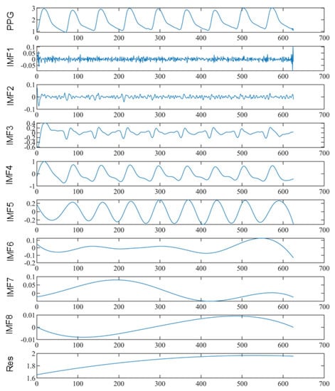
Figure 5.
EEMD decomposition of PPG.
In order to improve the training efficiency of the deep neural network prediction model, it is necessary to normalize each subsequence. The deviation standardization formula is selected for data normalization:
where: and are the maximum and minimum values in the sample sequence respectively, and is the normalized data.
Input the original PPG sequence and the IMF subsequences obtained after EEMD into the model for feature extraction. To better demonstrate the advantages of the expanded data set, CNN, CNN-LSTM, CNN-GRU, and TCN models with the same parameters are still used. The neural model results of each depth of the data set expanded by EEMD are shown in Table 3.
Table 3.
Results of each model on the dataset augmented with EEMD.
From Table 2 and Table 3, we can see that in the prediction of SBP, the expanded data set improves the performance of the four models, and the prediction result of TCN mmHg is still better than the other three models. In the prediction of DBP, the MAE of the CNN and TCN models is only reduced using the EEMD augmented dataset, and the model result of TCN is mmHg is also stronger than the other three models.
4.4. Model Performance Analysis and Evaluation
4.4.1. TCN Model Performance Analysis
In the experiment, to study the correlation between the estimated values of SBP and DBP and the true values of the test set, the author carried out the Bland–Altman consistency test and scatter plot analysis for the estimated values.
The Bland–Altman diagram is a key method to evaluate the consistency between two measurement methods. The 95% confidence interval boundary is set to [mean-1.96sd, mean + 1.96sd], where mean here represents the mean of the difference between the estimated value and the true value, and sd represents the standard deviation of the difference between the true value and the estimated value. The results of the consistency analysis of SBP and DBP are shown in Figure 6, the average errors between the estimated and target values are −0.48 mmHg and −0.41 mmHg, respectively.
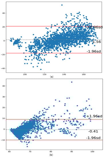
Figure 6.
Bland–Altman diagram of true value and estimated value; (a) SBP (b) DBP.
It can be seen from Figure 6 that within the confidence interval, both SBP and DBP show very superior performance. Under the 95% confidence interval, the statistical ranges of SBP and DBP are [−20.99, 17.97] and [−9.94, 9.12], respectively. Figure 7 presents a scatterplot of the true-predicted values of SBP and DBP. As can be seen, the correlation coefficients estimated by SBP and DBP are 0.9 and 0.81, respectively. This shows a solid positive correlation between the blood pressure target value and the estimated value.
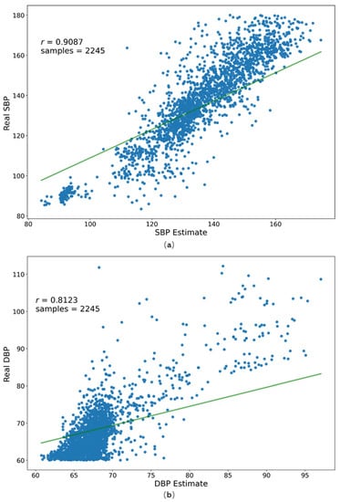
Figure 7.
Regression diagram of SBP (a) and DBP (b).
4.4.2. Evaluation of Model Performance Based on AAMI and BHS Standards
The AAMI standard requires that the ME and SD of blood pressure estimation and measurement equipment are less than 5 mmhg and 8 mmhg respectively. In the method proposed in this paper, the ME and SD of SBP and DBP estimation errors are −1.55 ± 9.92 mmHg and 0.41 ± 4.86 mmHg, respectively. The SD of SBP is 9.92, slightly higher than the AAMI standard, and the SDy of DBP meets the AAMI standard, which indicates that the estimation performance of DBP is good.
The British Hypertension Association Standard (BHS) requires that the blood pressure estimation and measurement equipment should be graded according to the cumulative frequency error percentage of the estimated result value, which is Grade A (60% < 5 mmHg; 85% < 10 mmHg; 95% < 15 mmHg), Grade B (50% < 5 mmHg; 75% < 10 mmHg; 90% < 15 mmHg), grade C (40% < 5 mmHg; 65% < 10 mmHg; 85% < 15 mmHg). See Table 4 for the standard evaluation of the BHS. The sample errors of 68.69% SBP and 78.31% DBP estimates are less than 5 mmHg, which means that they meet the Class A standard of BHS. However, when the threshold is 15, only 91.84% of SBP samples are less than 15 mmHg, so SBP meets the B standard of BHS. Similarly, the prediction of SBP by CNN and the hybrid neural networks CNN-LSTM and CNN-GRU has reached the B-level standard of BHS, and DBP has reached the A-level standard, but the overall effect of TCN is better. The data in UCI comes from the intensive care unit, and these abnormal data may affect the overall accuracy of the model.
Table 4.
Model performance evaluation based on BHS standard.
5. Conclusions
This paper proposes a continuous blood pressure estimation method based on TCN and uses PPG and decomposed IMF to train the model. This method explores the realization of high-precision daily continuous blood pressure monitoring. Using the IMF-added dataset allows the model to dig deeper into the original sequence characteristics, while the TCN model can effectively capture the internal correlation characteristics of the sequence, and then track the sequence change trend with high precision. In the dataset used in this paper, the estimates of SBP achieve a B grade and DBP a grade of A according to the BHS standard. Among the selected depth models of CNN, CNN-LSTM, and CNN-GRU, the prediction error of the TCN model is the lowest. Compared with EEMD-CCN and EEMD-CNN-RNN prediction models, the prediction error of EETCN is lower, and after joining IMF, the above four models have improved the accuracy of SBP prediction, and the two convolution neural network models in DBP prediction have better results. The results prove the potential of the proposed method in BP estimation. In future research, the deep neural network model can be trained on high-quality data sets; for example, data with higher sampling rates, signals of normal samples, and waveform signals can contain richer information. In addition, for the IMF decomposed by EEMD, it is possible to select the best IMF of M order and input the best IMF and PPG into the constructed deep neural network model to progress the forecast precision of the BP monitoring model.
Author Contributions
Conceptualization, K.Z. and Z.Y.; methodology, K.Z.; software, K.Z.; validation, K.Z., Y.P. and Z.Z.; formal analysis, K.Z.; investigation, K.Z.; resources, Z.Y.; data curation, Y.P.; writing—original draft preparation, K.Z.; writing—review and editing, K.Z.; visualization, Z.Z.; supervision, Y.P.; project administration, Z.Y.; funding acquisition, Z.Y. All authors have read and agreed to the published version of the manuscript.
Funding
This research was supported by National Natural Science Foundation of China (No: 62072296, 61672001) and Sub-Project of CST Forward Innovation Project (No. 18163ZT00500901).
Institutional Review Board Statement
Not applicable.
Informed Consent Statement
Not applicable.
Data Availability Statement
Data from open-source database.
Conflicts of Interest
The authors declare no conflict of interest.
References
- Amini, M.; Zayeri, F.; Salehi, M. Trend analysis of cardiovascular disease mortality, incidence, and mortality-to-incidence ratio: Results from global burden of disease study 2017. BMC Public Health 2021, 21, 401. [Google Scholar] [CrossRef] [PubMed]
- Umbrajkar, S.; Stankowski, R.V.; Rezkalla, S.; Kloner, R.A. Cardiovascular Health and Disease in the Context of COVID-19. Cardiol. Res. 2021, 12, 67. [Google Scholar] [CrossRef] [PubMed]
- Park, J.-U.; Kang, D.-W.; Erdenebayar, U.; Kim, Y.-J.; Cha, K.-C.; Lee, K.-J. Estimation of arterial blood pressure based on artificial intelligence using single earlobe photoplethysmography during cardiopulmonary resuscitation. J. Med. Syst. 2020, 44, 18. [Google Scholar] [CrossRef] [PubMed]
- Sharma, M.; Barbosa, K.; Ho, V.; Griggs, D.; Ghirmai, T.; Krishnan, S.K.; Hsiai, T.K.; Chiao, J.-C.; Cao, H. Cuff-less and continuous blood pressure monitoring: A methodological review. Technologies 2017, 5, 21. [Google Scholar] [CrossRef] [Green Version]
- O’Rourke, M.F. Time domain analysis of the arterial pulse in clinical medicine. Med. Biol. Eng. Comput. 2009, 47, 119–129. [Google Scholar] [CrossRef] [PubMed] [Green Version]
- Chen, S.; Ji, Z.; Wu, H.; Xu, Y.J. A non-invasive continuous blood pressure estimation approach based on machine learning. Sensors 2019, 19, 2585. [Google Scholar] [CrossRef] [Green Version]
- Chowdhury, M.H.; Shuzan, M.N.I.; Chowdhury, M.E.; Mahbub, Z.B.; Uddin, M.M.; Khandakar, A.; Reaz, M.B. Estimating blood pressure from the photoplethysmogram signal and demographic features using machine learning techniques. Sensors 2020, 20, 3127. [Google Scholar] [CrossRef]
- Xing, X.; Sun, M. Optical blood pressure estimation with photoplethysmography and FFT-based neural networks. Biomed. Opt. Express 2016, 7, 3007–3020. [Google Scholar] [CrossRef] [Green Version]
- Fujita, D.; Suzuki, A.; Ryu, K. PPG-based systolic blood pressure estimation method using PLS and level-crossing feature. Appl. Sci. 2019, 9, 304. [Google Scholar] [CrossRef] [Green Version]
- Zhang, Y.; Feng, Z. A SVM method for continuous blood pressure estimation from a PPG signal. In Proceedings of the 9th International Conference on Machine Learning and Computing, Singapore, 24–26 February 2017; pp. 128–132. [Google Scholar]
- Chen, Y.; Wen, C.; Tao, G.; Bi, M.; Li, G. Continuous and noninvasive blood pressure measurement: A novel modeling methodology of the relationship between blood pressure and pulse wave velocity. Ann. Biomed. Eng. 2009, 37, 2222–2233. [Google Scholar] [CrossRef]
- Lee, J.; Yang, S.; Lee, S.; Kim, H.C. Analysis of pulse arrival time as an indicator of blood pressure in a large surgical biosignal database: Recommendations for developing ubiquitous blood pressure monitoring methods. J. Clin. Med. 2019, 8, 1773. [Google Scholar] [CrossRef] [PubMed] [Green Version]
- Lin, W.-H.; Chen, F.; Geng, Y.; Ji, N.; Fang, P.; Li, G. Control, Towards accurate estimation of cuffless and continuous blood pressure using multi-order derivative and multivariate photoplethysmogram features. Biomed. Signal Process. Control 2021, 63, 102198. [Google Scholar] [CrossRef]
- Zhang, B.; Wei, Z.; Ren, J.; Cheng, Y.; Zheng, Z. An empirical study on predicting blood pressure using classification and regression trees. IEEE Access 2018, 6, 21758–21768. [Google Scholar] [CrossRef]
- Attarpour, A.; Mahnam, A.; Aminitabar, A.; Samani, H. Control, Cuff-less continuous measurement of blood pressure using wrist and fingertip photo-plethysmograms: Evaluation and feature analysis. Biomed. Signal Process. Control 2019, 49, 212–220. [Google Scholar] [CrossRef]
- Esmaelpoor, J.; Moradi, M.H.; Kadkhodamohammadi, A. Medicine, A multistage deep neural network model for blood pressure estimation using photoplethysmogram signals. Comput. Biol. Med. 2020, 120, 103719. [Google Scholar] [CrossRef]
- Ding, X.-R.; Zhang, Y.-T.; Liu, J.; Dai, W.-X.; Tsang, H.K. Continuous cuffless blood pressure estimation using pulse transit time and photoplethysmogram intensity ratio. IEEE Trans. Biomed. Eng. 2015, 63, 964–972. [Google Scholar] [CrossRef]
- Hannun, A.Y.; Rajpurkar, P.; Haghpanahi, M.; Tison, G.H.; Bourn, C.; Turakhia, M.P.; Ng, A.Y. Cardiologist-level arrhythmia detection and classification in ambulatory electrocardiograms using a deep neural network. Nat. Med. 2019, 25, 65–69. [Google Scholar] [CrossRef]
- Tanveer, M.S.; Hasan, M.K. Control, Cuffless blood pressure estimation from electrocardiogram and photoplethysmogram using waveform based ANN-LSTM network. Biomed. Signal Process. Control 2019, 51, 382–392. [Google Scholar] [CrossRef] [Green Version]
- Paviglianiti, A.; Randazzo, V.; Villata, S.; Cirrincione, G.; Pasero, E. A Comparison of Deep Learning Techniques for Arterial Blood Pressure Prediction. Cogn. Comput. 2021, 1–22. [Google Scholar] [CrossRef]
- Su, P.; Ding, X.-R.; Zhang, Y.-T.; Liu, J.; Miao, F.; Zhao, N. Long-term blood pressure prediction with deep recurrent neural networks. In Proceedings of the 2018 IEEE EMBS International Conference on Biomedical & Health Informatics (BHI), Las Vegas, NV, USA, 4–7 March 2018; pp. 323–328. [Google Scholar]
- Lee, S.; Chang, J.-H. Oscillometric blood pressure estimation based on deep learning. IEEE Trans. Ind. Inform. 2016, 13, 461–472. [Google Scholar] [CrossRef]
- Rong, M.; Li, K. Control, A multi-type features fusion neural network for blood pressure prediction based on photoplethysmography. Biomed. Signal Process. Control 2021, 68, 102772. [Google Scholar] [CrossRef]
- Hsu, Y.-C.; Li, Y.-H.; Chang, C.-C.; Harfiya, L.N. Generalized deep neural network model for cuffless blood pressure estimation with photoplethysmogram signal only. Sensors 2020, 20, 5668. [Google Scholar] [CrossRef] [PubMed]
- Lee, D.; Kwon, H.; Son, D.; Eom, H.; Park, C.; Lim, Y.; Seo, C.; Park, K. Beat-to-beat continuous blood pressure estimation using bidirectional long short-term memory network. Sensors 2020, 21, 96. [Google Scholar] [CrossRef] [PubMed]
- Irie, K.; Tüske, Z.; Alkhouli, T.; Schlüter, R.; Ney, H. LSTM, GRU, highway and a bit of attention: An empirical overview for language modeling in speech recognition. Interspeech 2016, 2016, 3519–3523. [Google Scholar]
- Yan, J.; Mu, L.; Wang, L.; Ranjan, R.; Zomaya, A.Y. Temporal convolutional networks for the advance prediction of ENSO. Sci. Rep. 2020, 10, 8055. [Google Scholar] [CrossRef]
- Jarrett, D.; Yoon, J.; van der Schaar, M. Dynamic prediction in clinical survival analysis using temporal convolutional networks. IEEE J. Biomed. Health Inform. 2019, 24, 424–436. [Google Scholar] [CrossRef]
- Sun, L.; Jia, K.; Yeung, D.-Y.; Shi, B.E. Human action recognition using factorized spatio-temporal convolutional networks. In Proceedings of the IEEE International Conference on Computer Vision, Washington, DC, USA, 7–13 December 2015; pp. 4597–4605. [Google Scholar]
- Bai, S.; Kolter, J.Z.; Koltun, V. An empirical evaluation of generic convolutional and recurrent networks for sequence modeling. arXiv 2018, arXiv:1803.01271. [Google Scholar]
- Cheng, J.; Xu, Y.; Song, R.; Liu, Y.; Li, C.; Chen, X. Medicine, Prediction of arterial blood pressure waveforms from photoplethysmogram signals via fully convolutional neural networks. Comput. Biol. Med. 2021, 138, 104877. [Google Scholar] [CrossRef]
- Slapničar, G.; Mlakar, N.; Luštrek, M. Blood pressure estimation from photoplethysmogram using a spectro-temporal deep neural network. Sensors 2019, 19, 3420. [Google Scholar] [CrossRef] [Green Version]
- Wang, D.; Yang, X.; Liu, X.; Fang, S.; Ma, L.; Li, L. Photoplethysmography based stratification of blood pressure using multi-information fusion artificial neural network. In Proceedings of the IEEE/CVF Conference on Computer Vision and Pattern Recognition Workshops, Seattle, WA, USA, 14–19 June 2020; pp. 276–277. [Google Scholar]
- Viunytskyi, O.; Shulgin, V.; Sharonov, V.; Totsky, A. Non-invasive cuff-less measurement of blood pressure based on machine learning. In Proceedings of the 2020 IEEE 15th International Conference on Advanced Trends in Radioelectronics, Telecommunications and Computer Engineering (TCSET), Lviv-Slavske, Ukraine, 25–29 February 2020; pp. 203–206. [Google Scholar]
- Monte-Moreno, E. Non-invasive estimate of blood glucose and blood pressure from a photoplethysmograph by means of machine learning techniques. Artif. Intell. Med. 2011, 53, 127–138. [Google Scholar] [CrossRef]
- Khalid, S.G.; Zhang, J.; Chen, F.; Zheng, D. Blood pressure estimation using photoplethysmography only: Comparison between different machine learning approaches. J. Healthc. Eng. 2018, 2018, 1548647. [Google Scholar] [CrossRef] [PubMed] [Green Version]
- Hu, Q.; Deng, X.; Wang, A.; Yang, C. A novel method for continuous blood pressure estimation based on a single-channel photoplethysmogram signal. Physiol. Meas. 2020, 41, 125009. [Google Scholar] [CrossRef] [PubMed]
- Mao, J.; Jain, A.K. Artificial neural networks for feature extraction and multivariate data projection. IEEE Trans. Neural Netw. 1995, 6, 296–317. [Google Scholar] [PubMed]
- Baek, S.; Jang, J.; Yoon, S. End-to-end blood pressure prediction via fully convolutional networks. IEEE Access 2019, 7, 185458–185468. [Google Scholar] [CrossRef]
- El-Hajj, C.; Kyriacou, P.A. Control, Deep learning models for cuffless blood pressure monitoring from PPG signals using attention mechanism. Biomed. Signal Process. Control 2021, 65, 102301. [Google Scholar] [CrossRef]
- Wang, C.; Yang, F.; Yuan, X.; Zhang, Y.; Chang, K.; Li, Z. An end-to-end neural network model for blood pressure estimation using ppg signal. In Artificial Intelligence in China; Springer: Berlin/Heidelberg, Germany, 2020; pp. 262–272. [Google Scholar]
- Zhao, W.; Gao, Y.; Ji, T.; Wan, X.; Ye, F.; Bai, G. Deep temporal convolutional networks for short-term traffic flow forecasting. IEEE Access 2019, 7, 114496–114507. [Google Scholar] [CrossRef]
- Song, J.; Xue, G.; Pan, X.; Ma, Y.; Li, H. Hourly heat load prediction model based on temporal convolutional neural network. IEEE Access 2020, 8, 16726–16741. [Google Scholar] [CrossRef]
- Lan, H.; Yin, H.; Hong, Y.-Y.; Wen, S.; David, C.Y.; Cheng, P. Day-ahead spatio-temporal forecasting of solar irradiation along a navigation route. Appl. Energy 2018, 211, 15–27. [Google Scholar] [CrossRef]
- Chen, Y.; Dong, Z.; Wang, Y.; Su, J.; Han, Z.; Zhou, D.; Zhang, K.; Zhao, Y.; Bao, Y. Management, Short-term wind speed predicting framework based on EEMD-GA-LSTM method under large scaled wind history. Energy Convers. Manag. 2021, 227, 113559. [Google Scholar] [CrossRef]
- Huang, N.E.; Shen, Z.; Long, S.R.; Wu, M.C.; Shih, H.H.; Zheng, Q.; Yen, N.-C.; Tung, C.C.; Liu, H.H. The empirical mode decomposition and the Hilbert spectrum for nonlinear and non-stationary time series analysis. Proc. R. Soc. Lond. Ser. A Math. Phys. Eng. Sci. 1998, 454, 903–995. [Google Scholar] [CrossRef]
- Wu, Z.; Huang, N.E. Ensemble empirical mode decomposition: A noise-assisted data analysis method. Adv. Adapt. Data Anal. 2009, 1, 1–41. [Google Scholar] [CrossRef]
- Hewage, P.; Behera, A.; Trovati, M.; Pereira, E.; Ghahremani, M.; Palmieri, F.; Liu, Y. Temporal convolutional neural (TCN) network for an effective weather forecasting using time-series data from the local weather station. Soft Comput. 2020, 24, 16453–16482. [Google Scholar] [CrossRef] [Green Version]
- He, K.; Zhang, X.; Ren, S.; Sun, J. Deep residual learning for image recognition. In Proceedings of the IEEE conference on Computer Vision and Pattern Recognition, Las Vegas, NV, USA, 27–30 June 2016; pp. 770–778. [Google Scholar]
- Kachuee, M.; Kiani, M.M.; Mohammadzade, H.; Shabany, M. Cuff-less high-accuracy calibration-free blood pressure estimation using pulse transit time. In Proceedings of the 2015 IEEE International Symposium on Circuits and Systems (ISCAS), Lisbon, Portugal, 24–27 May 2015; pp. 1006–1009. [Google Scholar]
Publisher’s Note: MDPI stays neutral with regard to jurisdictional claims in published maps and institutional affiliations. |
© 2022 by the authors. Licensee MDPI, Basel, Switzerland. This article is an open access article distributed under the terms and conditions of the Creative Commons Attribution (CC BY) license (https://creativecommons.org/licenses/by/4.0/).