Article

Metaheuristic Optimization-Based Path Planning and Tracking of Quadcopter for Payload Hold-Release Mission

Department of Electrical and Electronics Engineering, Zonguldak Bülent Ecevit University, 67100 Zonguldak, Turkey
*
Author to whom correspondence should be addressed.
Electronics 2022, 11(8), 1208; https://doi.org/10.3390/electronics11081208
Submission received: 12 March 2022 / Revised: 6 April 2022 / Accepted: 8 April 2022 / Published: 11 April 2022
(This article belongs to the Topic Artificial Intelligence and Sustainable Energy Systems)

Abstract

:
Under harsh geographical conditions where manned flight is not possible, the ability of the unmanned aerial vehicle (UAV) to successfully carry out the payload hold–release mission by avoiding obstacles depends on the optimal path planning and tracking performance of the UAV. The ability of the UAV to plan and track the path with minimum energy and time consumption is possible by using the flight parameters. This study performs the optimum path planning and tracking using Harris hawk optimization (HHO)–grey wolf optimization (GWO), a hybrid metaheuristic optimization algorithm, to enable the UAV to actualize the payload hold–release mission avoiding obstacles. In the study, the hybrid HHO–GWO algorithm, which stands out with its avoidance of local minima and speed convergence, is used to successfully obtain the feasible and effective path. In addition, the effect of the mass change uncertainty of the UAV on optimal path planning and tracking performance is determined. The effectiveness of the proposed approach is tested by comparing it with the metaheuristic swarm optimization algorithms such as particle swarm optimization (PSO) and GWO. The experimental results obtained indicate that the proposed algorithm generates a fast and safe optimal path without becoming stuck with local minima, and the quadcopter tracks the generated path with minimum energy and time consumption.

1. Introduction

Path planning and tracking are the main tasks studied for unmanned vehicles, especially unmanned aerial vehicles (UAVs), unmanned ground vehicles, and unmanned underwater vehicles [1,2,3,4]. UAVs, which have been used extensively in defense industry and academic studies in recent years, perform tasks such as surveillance, target tracking, search and rescue, and payload transportation [4,5,6,7]. The obstacles and their positions in the region where UAVs will operate play an important role in the effective operation of UAVs [8]. Establishing a safe path by determining the risky areas in military operation and natural disaster areas, following the path that has been generated, and releasing the payloads to the predefined regions are critical for the successful performance of the mission [9]. In this study, a new path planning and tracking algorithm based on metaheuristic optimization is developed for the payload hold–release task by avoiding the obstacles at the target points defined around the planned path.
A path planning and tracking is required for the UAV to safely reach the target location from the starting location depending on certain restriction conditions such as minimum flight distance and time [10]. UAVs may be exposed to inconvenient land and weather conditions while performing critical tasks. UAVs try to overcome this problem with their maneuverability and altitude capabilities [1]. This situation causes the UAV to consume more energy [11]. In the presence of obstacles and constraints, optimal path planning is required for the UAV to safely follow the specified path with minimum energy and time consumption [12,13]. The UAV path planning problem is a complex optimization problem that requires efficient algorithms to solve. This optimization problem can be solved with classical algorithms as well as by using quite efficient metaheuristic algorithms. Simple path planning for UAV is performed with the Voroni diagram algorithm [14], the probabilistic roadmaps algorithm [15], the A* algorithm [16], and rapidly discovered tree-based algorithms [17]. However, since the kinematic and dynamic constraints of the UAV are rarely considered, these algorithms are generally not preferred in practical applications. In recent years, various approaches have been proposed for the autonomous path planning of the UAV, including meta-heuristic optimization algorithms. In [18], modeling of the battery performance of the UAV is emphasized. A multi-variable linear regression model has been created for the minimum energy consumption of the UAV on the specified path. The generated energy consumption model is used as a fitness function in the optimization algorithm. The performance of the proposed algorithm has been verified with various scenarios for the minimum energy consumption of the UAV. In [19], a path planning algorithm based on k-degree smoothing is proposed to define the coordinated path planning of the UAV in a safe and efficient manner. In the study, a k-degree smoothing method that aims to obtain a safer path using the ant colony optimization (ACO) algorithm [20] is presented. The proposed algorithm draws attention with its slow convergence speed and high probability of being stuck to local optima. In order to deal with these problems, a hybrid optimization algorithm obtained by combining maximum–minimum ACO (MMACO) and Cauchy mutant (CM) operators is recommended in [21]. As paths with faster convergence speed and better solution optimization are preferred in practical applications, swarm-based bio-inspiring optimization algorithms with low computational complexity and high computational speed are used extensively. In [22], an improved particle swarm optimization (PSO) algorithm has been proposed to achieve faster convergence speed and better solution optimization in the path planning of the UAV. The performance of the algorithm has been tested on various UAVs under many environmental constraints with Monte Carlo simulations. In [23], the 3D path planning problem of the UAV in the presence of obstacles is solved with the grey wolf optimization (GWO) algorithm [24] and the performance of the proposed algorithm is compared with metaheuristic algorithms such as PSO, the whale optimization algorithm (WOA), and the sine cosine algorithm (SCA). In the literature, metaheuristic optimization algorithms play an important role in solving different engineering problems, as well as path planning and tracking [25,26,27].
UAVs may encounter various obstacles while performing specified missions by sticking to a path. In [28], an obstacle avoidance algorithm based on ellipsoid geometry is proposed for the UAV to remain loyal to its original path and avoid the obstacles in its environment by creating waypoints in the presence of obstacles that obstruct the UAV flight path. The search for an avoidance path in the proposed algorithm is based on the use of ellipsoid geometry as a limited region containing the obstacle. Considering the geometry of the defined obstacle, a limited ellipsoid zone is created, and new crossing points are calculated within this zone. A convolutional neural network (CNN) approach based on depth estimation using molecular camera data to enable the quadrotor UAV to independently avoid collisions with obstacles in unknown and unstructured environments is presented in [29]. In [30], a new algorithm has been proposed that analytically calculates the path efficiently and effectively to create an environment map with a path without collision. In the developed algorithm, an initial path is created by the intersection of two 3D surfaces. Each obstacle position is shaped around the obstacles by adding a radial function to one of the two surfaces. The developed algorithm ensures that the intersection between deformed surfaces does not intersect with obstacles. The algorithm provides that the safe path is created in real time in the UAV’s path tracking. In [31], every point in the motion environment is scanned with the 2D lidar on the UAV and the position of the UAV is estimated using the point cloud correction method. Unlike many studies with lidar, the effects of motion on the point cloud have been taken into account. In the proposed algorithm, point cloud features obtained by laser radar are extracted and a clustering is made based on relative distance and density. A robust nonlinear flight controller framework with six dimensional force and torque estimators that includes a model predictive controller (MPC)-based trajectory plan that considers the trajectory planning problem as an optimal control problem with nonlinear obstacle avoiding limitations is proposed in [32].
The ability of the UAV, which has a payload transportation system, to move around the reference trajectory and hold payloads from a certain point and to release payloads to specified targets with minimum error makes the UAV important for critical missions. In releasing the payloads to the specified targets, the UAV should be able to determine the path on its own or stay loyal to the specified path. In [33], neural-network-based real-time UAV control is performed in order to release the payloads to the marked targets by following a certain path with minimum error. The controller structure includes feature extraction and selection stages. In order for the UAV to release the payloads on the predetermined coordinates with the highest accuracy, the full mathematical model of the UAV, as well as the model of the payload transportation system, is needed. In [34], both the dynamic model parameters and the payload transportation system model of the UAV are handled together with the controller approach based on the law of feedback linearization. It is stated that the stabilization of the UAV, especially when releasing payload, is improved with the proposed controller approach. The controller scheme robust to payload changes in various weights is presented in [35]. The proposed controller provides the stabilization of the UAV in the suspended position by compensating the weight changes in the UAV with payload transportation system. In [36], an optimization-based controller algorithm has been developed for the UAV moving around a certain trajectory to make minimum oscillation at maximum payload. It is emphasized that the developed algorithm performs optimal control, especially in maneuvers.
In this study, a new metaheuristic-optimization-based path planning and tracking algorithm with a very high convergence speed is proposed to the UAV with payload transportation system in order to plan a path by avoiding obstacles under constraints such as mass uncertainty, unknown parameters, and unmeasurable external disturbances and to release the payloads to the target points with minimum error while staying loyal to path. The proposed algorithm is robust as it copes with unknown system dynamics and adverse environmental factors. The main contributions of this study are that the new hybrid Harris hawk optimization (HHO)–GWO algorithm for path planning is proposed, the new path planning and tracking control strategy is developed together, and the path-tracking performance of the quadcopter in payload hold–release mission has been analyzed. In addition, the positional error due to the mass uncertainty can be minimized by the proposed control strategy, as well as the energy function. The results of the study are shown that the mass uncertainty and energy of quadcopter during payload hold–release mission have been minimized using the new proposed path planning and tracking algorithm.
The remainder of this paper is organized as follows. The dynamic model of the quadrotor UAV used in the study is given in Section 2. The proposed controller approach for the path planning and tracking of the UAV is introduced in Section 3, including GWO and HHO algorithms. The generated maps are presented in Section 4. The results obtained with the proposed model are discussed in Section 5. Finally, in Section 6, the main results of the study, and future work are highlighted.

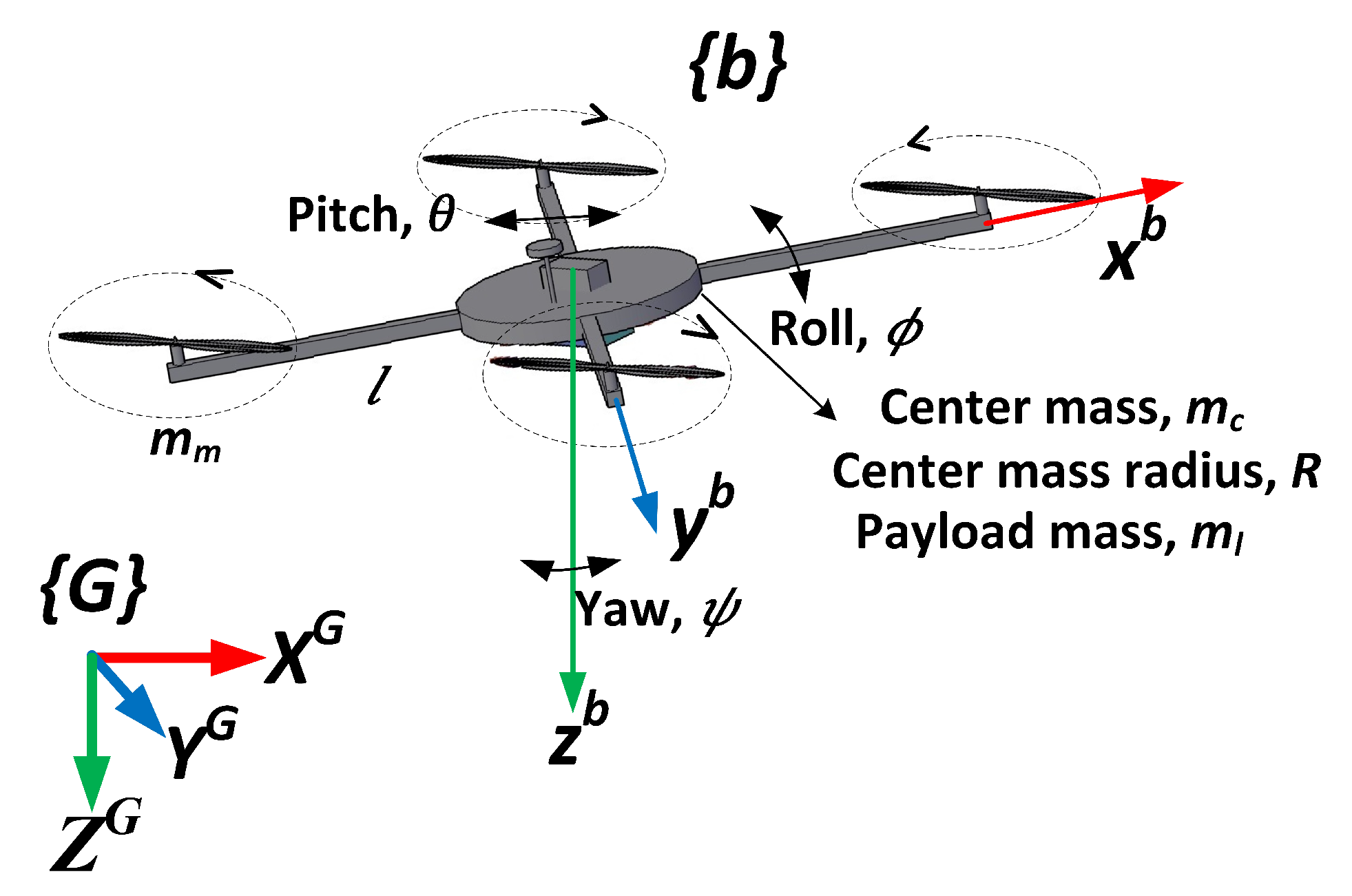
2. Dynamic Model of Quadcopter

Quadcopter is an underactuated type of UAV with four motors and six degrees of freedom (three translational and three rotations) and capable of landing and taking off in limited areas [37]. The evaluation of translation and rotation dynamics together in the motion control of a quadcopter is an important control problem. In the solution of this control problem, it is very important to take into account the non-linear parameters in the dynamics of the quadcopter. The main components of the quadcopter, Euler angles (roll, pitch, yaw), body frame, and global frame are illustrated in Figure 1.
The following parameters:
  • The frame of the quadcopter is symmetrical and the center of gravity is in the middle of the fuselage;
  • The thrust and friction of each motor of a quadcopter is proportional to the square of their motor speed;
  • Moment of inertia of the propellers;
  • During the flight of the qudcopter, the Earth is flat and non-rotating.
are assumed in the model of quadcopter [38]. Position changes during quadcopter flight are measured in the frame, accelerometer, and gyro values are measured in the body frame. For this reason, it is necessary to define the transformations between body and coordinate systems. In this study, c o s ( . ) , s i n ( . ) , and t a n ( . ) are represented by c ( . ) , s ( . ) , and t ( . ) , respectively. Considering these transformations, the velocity expression in the frame is obtained by using the velocity in body frame as:
X ˙ G Y ˙ G Z ˙ G = c ( ψ ) c ( θ ) c ( ψ ) s ( ϕ ) s ( θ ) c ( ϕ ) s ( ψ ) c ( ϕ ) c ( ψ ) s ( θ ) + s ( ϕ ) s ( ψ ) s ( ψ ) c ( θ ) s ( ϕ ) s ( ψ ) s ( θ ) + c ( ϕ ) c ( ψ ) c ( ϕ ) s ( ψ ) s ( θ ) c ( ψ ) s ( ϕ ) s ( θ ) c ( θ ) s ( ϕ ) c ( ϕ ) c ( θ ) x ˙ b y ˙ b z ˙ b
where X ˙ G , Y ˙ G , Z ˙ G velocities (m/s) ( X , Y , Z ) in global frame, ϕ , θ , ψ (roll, pitch, yaw angles), (rad), and x ˙ b , y ˙ b , z ˙ b velocities ( X , Y , Z ) in the body frame [38,39]. The equations of motion of the quadcopter consist of two main components, dynamic and kinematic. Dynamic components explain the motion of the quadcopter according to Newton’s second laws, while kinematic components explain the quadcopter’s transformation equations. The rotational kinematics of the quadcopter describe the relationship between the angular rate and Euler angles. According to this rotation kinematics, since the angular rate is given in the body frame and the Euler angles are given in the frame, the relation between each other is obtained as:
ϕ ˙ θ ˙ ψ ˙ = 1 s ( ϕ ) t ( θ ) c ( ϕ ) t ( θ ) 0 c ( ϕ ) s ( ϕ ) 0 s ( ϕ ) c ( θ ) c ( ϕ ) c ( θ ) p q r
by using the transformation matrix, where p, q, r roll, pitch, yaw rates (rad/s) and ϕ ˙ , θ ˙ , ψ ˙ , and (rad/s) time derivatives of Euler angles, respectively [38,40]. Translational s describes the linear motion of all forces acting on the quadcopter during flight according to the coordinate frame. Equations of motion resulting from translational s of the quadcopter are obtained as in Equation (3), according to Newton’s second law:
X ¨ G Y ¨ G Z ¨ G = 1 m ( [ c ( ϕ ) c ( ψ ) s ( θ ) + s ( ϕ ) s ( ψ ) ] u 1 K d x X ˙ G ) 1 m ( [ c ( ϕ ) s ( ψ ) s ( θ ) c ( ψ ) s ( ϕ ) ] u 1 K d y Y ˙ G ) 1 m ( [ c ( ϕ ) c ( θ ) ] u 1 K d z Z ˙ G ) + g
where X ¨ G , Y ¨ G , Z ¨ G accelerations (m/s 2 ) X , Y , Z in the coordinates, m mass of quadcopter (kg), K d x , K d y , K d z drag coefficients, X ˙ G , Y ˙ G , Z ˙ G velocities X , Y , Z in the coordinates, and u 1 is total thrust of all motors, respectively [41]. The rotational s of quadcopter describes the relationship:
ϕ ¨ θ ¨ ψ ¨ = [ ( J y J z ) q r J r q ( w 1 w 2 + w 3 w 4 ) + l K T u 2 ] J x [ ( J z J x ) p r + J r p ( w 1 w 2 + w 3 w 4 ) + l K T u 3 ] J y [ ( J x J y ) p q + K d u 4 ] J z
between the second derivatives of Euler angles ( ϕ ¨ , θ ¨ , ψ ¨ ) (rad/s 2 ) on each axis depending on the square of its motor speeds ( w 1 , w 2 , w 3 , w 4 ) (rad/s), namely, torques, and  J x , J y , and J z (kg m 2 ) quadcopter moments of ineartia on each axis. u 2 refers roll control input, u 3 describes pitch control input, u 4 indicates yaw control input, K T is the thrust coefficient,  K d is the drag torque proportionality constant, and l is the arm length of quadcopter (m) as in Equation (4) [38,41]. The quadcopter moments of inertia on each axis and mass of quadcopter are expressed [41]:
J x = J y = 2 ( m c + m l ) R 2 5 + 2 l 2 m m J z = 2 ( m c + m l ) R 2 5 + 4 l 2 m m m = 4 m m + m c + m l
where m c is the center mass of quadcopter (kg), R is the radius of center mass (m), m m is the motor mass (kg), and m l is the payload mass (kg). In this study, the total mass in the system model of the quadcopter is changed during the payload hold–release mission depending on the weight of the payload carried, and the moment of inertia in each axis is directly related to this mass change. To summarize, the dynamic and kinematic model of the quadcopter with six degrees of freedom is represented as Equations (1)–(4). The relationship between motor speeds and control variables is defined as:
u 1 u 2 u 3 u 4 = K T K T K T K T 0 l K T 0 l K T l K T 0 l K T 0 K d K d K d K d w 1 2 w 2 2 w 3 2 w 4 2
Note that the control variables are directly proportional to the squares of the motor speeds.

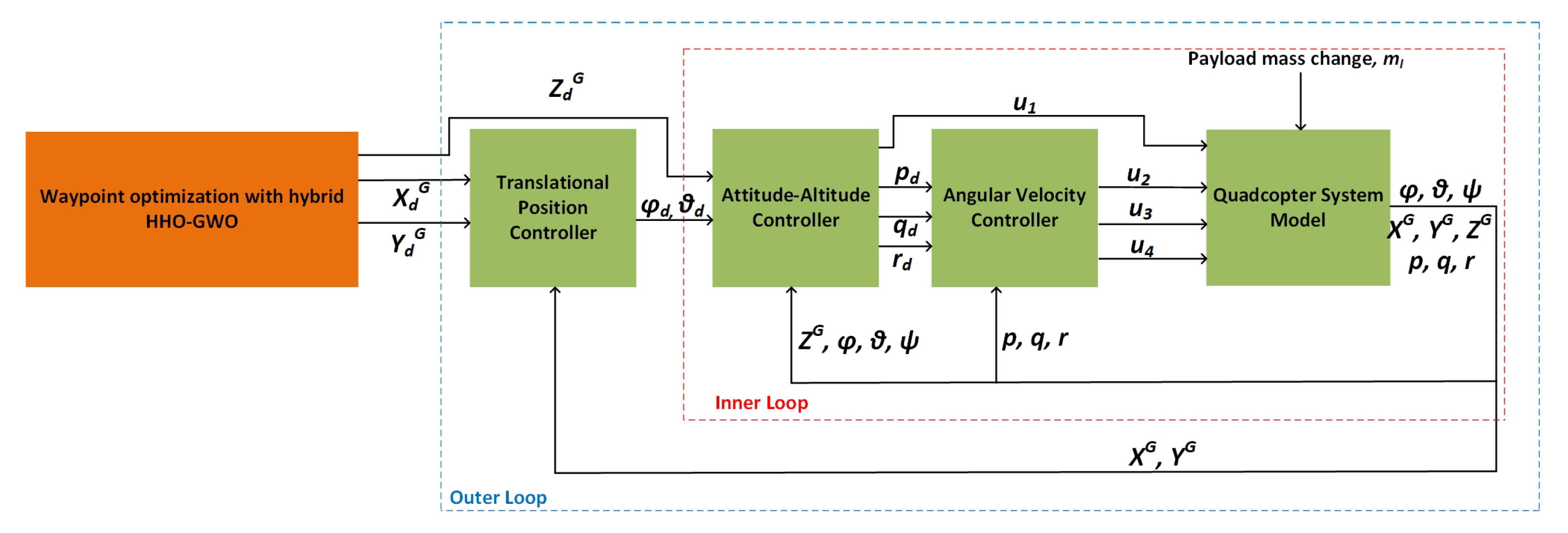
3. Proposed Control Approach for Path Planning and Tracking

The control strategy of this study consists of path planning and tracking. The hybrid HHO–GWO algorithm, which has high convergence speed and swarm intelligence that can avoid local minimum points, is proposed in this study in determining the optimum path. The path planning performances of the proposed optimization algorithm are compared with metaheuristic optimization algorithms such as PSO and GWO. The payload hold–release path determined by these optimization algorithms is generated with the shortest distance and avoiding the areas where there are obstacles. By analyzing the multi-objective function with metaheuristic optimization algorithms, waypoints to be followed by the UAV are generated. As seen in Figure 2, after the waypoints that the quadcopter are to follow are generated, the following of these waypoints, namely, the path tracking, is carried out with controller in a nested structure. The main idea of the study is that a new control strategy is proposed to carry out path planning and tracking together for the quadcopter’s payload hold–release mission. The section includes not only controller design of quadcopter but also metaheuristic algorithms such as PSO, GWO, and HHO.

3.1. Controller Design

The control strategy proposed in this study consists of two main steps: path planning and the tracking of the path. Path planning, which is the first step of the control strategy, is the process of determining the waypoints that the quadcopter is desired to track during payload transportation mission. Metaheuristic optimization algorithms such as PSO, GWO, and hybrid HHO–GWO are used to identify these waypoints. After determining the waypoints that the quadcopter is desired to track, path tracking is performed as the second step of control strategy. The path tracking process consists of four control structures: translational position, attitude–altitude, angular velocity controllers, and the system model of quadcopter. This path tracking controller is nested with each other. The motion control on the X and Y axes, attitude–altitude control and the angular velocity control of quadcopter are performed on the outer part, the inner part, and the innermost part, respectively. In the study, noise that occurs as a disruptive effect in attitude, altitude, and angular velocity control is suppressed by Kalman filter [42]. The position errors of quadcopter in X, Y, and Z axes are indicated as:
e x = X d G X G e y = Y d G Y G e z = Z d G Z G
where e x , e y , and e z refer the position errors; X d G , Y d G , and Z d G denote the desired positions; and  X G , Y G , and Z G define the measured positions in the X, Y, and Z axes, respectively. The errors of quadcopter in orientation angles are specified as:
e ϕ = ϕ d ϕ e θ = θ d θ e ψ = ψ d ψ
where e ϕ , e θ , and e ψ describe the orientation errors; ϕ d , θ d , and ψ d define the desired orientation angles; and  ϕ , θ , and ψ represent the measured orientation angles in the roll, pitch, and yaw angle, respectively. The angular velocity error is stated as:
e p = p d p e q = q d q e r = r d r
where e p , e q , and e r are the angular velocity errors; p d , q d , and r d define the desired angular velocity; and p, q, and r express the measured angular velocity along x b , y b , z b , respectively.

3.1.1. Translational Position Control

This controller is responsible for minimizing the measurement difference obtained from the desired position and the quadcopter system model output. As specified in Equations (10) and (11):
θ d ( t ) = K P X e x ( t ) + K I X 0 t e x ( τ ) d τ + K D X e ˙ x ( t )
ϕ d ( t ) = K P Y e y ( t ) + K I Y 0 t e y ( τ ) d τ + K D Y e ˙ y ( t )
the desired roll and pitch values are identified by the translational position controller as a result of the minimization of this error with the proportional–integral–derivative (PID) controller, and where K P X , K I X , K D X express PID gains that control the movement of the quadcopter in the X position, and K P Y , K I Y , K D Y indicate PID gains that control the movement of quadcopter in the Y position, respectively. The inputs of the translational position controller are desired the position ( X d G , Y d G ), the output of the quadcopter system model ( X G , Y G ), and the controller’s output are the desired pitch ( θ d ) and roll angles ( ϕ d ). The proposed controller also performs the tracking of waypoints specified in the X , Y plane with metaheuristic path planning algorithms [38].

3.1.2. Attitude–Altitude Control

The height and orientation angles (roll, pitch, yaw) of the quadcopter are controlled by the attitude–altitude controller. As stated in Equations (12)–(15):
u 1 ( t ) = 1 c o s ( ϕ ) c o s ( θ ) ( K P Z e z ( t ) + K I Z 0 t e z ( τ ) d τ + K D Z d e z ( t ) d t + m g )
p d ( t ) = K P ϕ e ϕ ( t ) + K I ϕ 0 t e ϕ ( τ ) d τ + K D ϕ d e ϕ ( t ) d t
q d ( t ) = K P θ e θ ( t ) + K I θ 0 t e θ ( τ ) d τ + K D θ d e θ ( t ) d t
r d ( t ) = K P ψ e ψ ( t ) + K I ψ 0 t e ψ ( τ ) d τ + K D ψ d e ψ ( t ) d t
K P Z , K I Z , K D Z express PID gains that control the movement of quadcopter in the Z position; K P ϕ , K I ϕ , K D ϕ specify PID gains that control the roll angle; K P θ , K I θ , K D θ describe PID gains that control the pitch angle; K P ψ , K I ψ , K D ψ denote PID gains that control the yaw angle. The inputs of the controller are desired and measured height, roll, pitch, and yaw angles; the outputs are u 1 ; and the desired angular velocities are ( p d , q d , r d ). u 1 obtained at the controller output is input into the quadcopter system, and this control variable enables the quadcopter to increase [38].

3.1.3. Angular Velocity Control

This controller performs angular velocity control, the main task of the controller is the minimization of error between desired and measured angular velocity components. The angular velocity control is denoted as:
u 2 ( t ) = K P P e p ( t ) + K I P 0 t e p ( τ ) d τ + K D P d e p ( t ) d t
u 3 ( t ) = K P Q e q ( t ) + K I Q 0 t e q ( τ ) d τ + K D Q d e q ( t ) d t
u 4 ( t ) = K P R e r ( t ) + K I R 0 t e r ( τ ) d τ + K D R d e r ( t ) d t
where K P P , K I P , K D P express PID gains that control the angular velocity along x b ; K P Q , K I Q , K D Q indicate PID gains that control the angular velocity along y b ; and K P R , K I R , K D R refer to PID gains that control the angular velocity along z b . The outputs of controller constitute the orientation control variables ( u 2 , u 3 , u 4 ) of the quadcopter [38].

3.1.4. Motor Control

Using the height and orientation control variables obtained from attitude–altitude and angular velocity controller outputs, the angular velocities required for the motors are obtained as in Equations (19) and (20) [38]. Thus, the thrust required for the movement of the quadcopter in the specified path is obtained by controlling the speed of the motors w i , i = 1 , 2 , 3 , 4 as:
w 1 2 = u 1 4 K T + u 3 2 l K T + u 4 4 K d w 2 2 = u 1 4 K T u 2 2 l K T u 4 4 K d
w 3 2 = u 1 4 K T u 3 2 l K T + u 4 4 K d w 4 2 = u 1 4 K T + u 2 2 l K T u 4 4 K d
The power consumed by each motor of quadcopter is indicated as:
P m k = P h k = ( 2 ρ A p ) ( K v K τ K t ) 3 w k 3 k = 1 , 2 , 3 , 4
where P m k denotes the power consumed by the kth motor, P h k explains the hovering power consumed by the kth motor, ρ is air density (kg/m 3 ), A p refers to the propeller cross-section (m 2 ), K v is the back electromotive force (EMF) constant, K τ is the torque proportionality constant, and K T is the thrust coefficient.

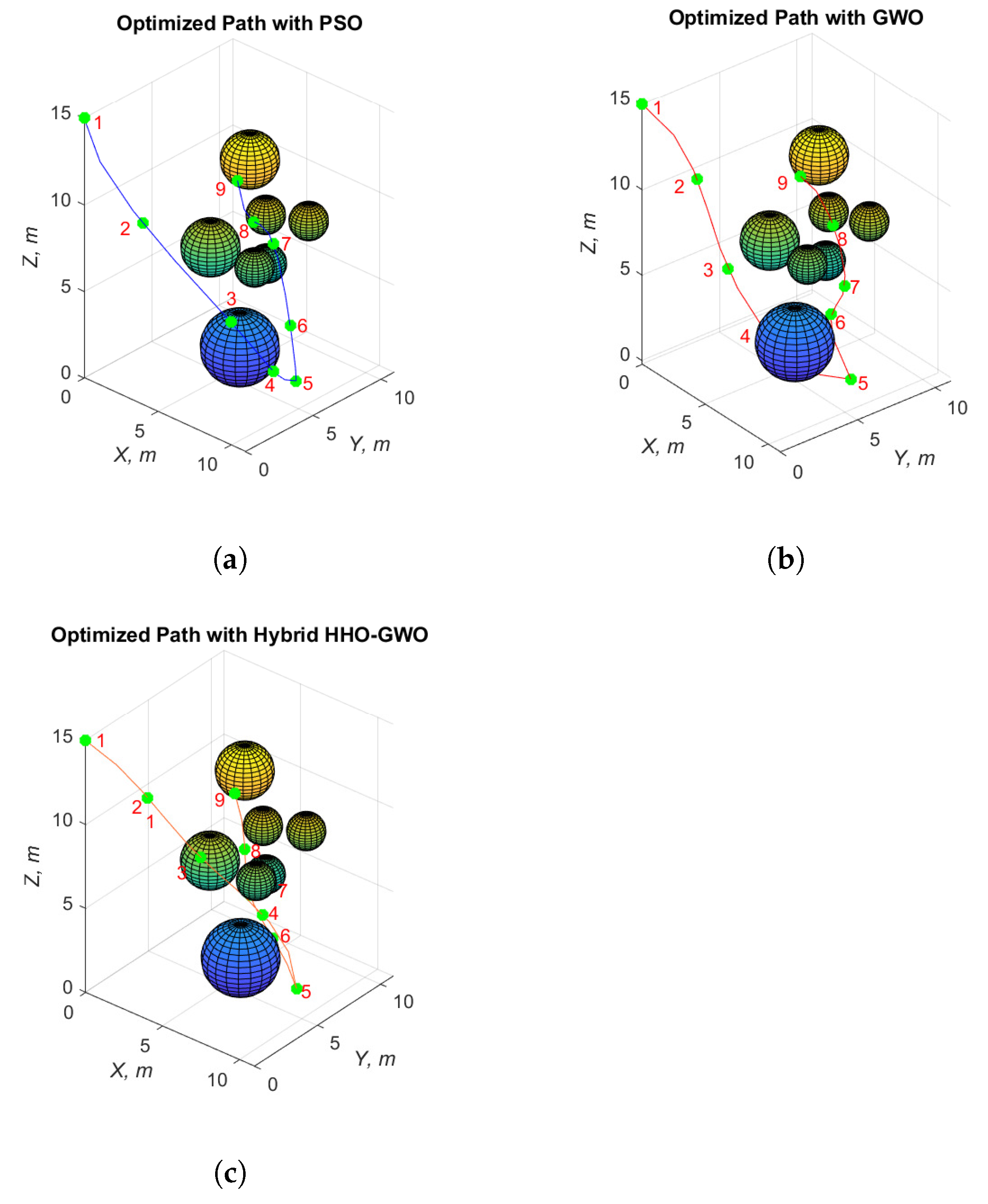
3.2. Three-Dimensional Path Planning Model of the Quadcopter

The 3D path planning algorithm proposed in this study is operated to define the optimum path by avoiding the obstacle region after the starting and ending point are determined. There are two limit values of the objective function, the starting ( x s , y s , z s ) and the ending points ( x t , y t , z t ). The number of waypoints to be generated, including starting, ending, payload hold, and payload release points, are entered. Afterwards, the locations of the spherical barriers on the map are defined as central positions ( x o b s , y o b s , z o b s ) and the radius ( r o b s ), and these locations are given as an input to the algorithm. The 3D path-planning algorithm presented in this study consists of three different objective functions. In the first part, the length of the generated path is indicated as:
d = i = 1 N p 1 d x i 2 + d y i 2 + d z i 2
where d x , d y , d z are the infinitesimal lengths traversed by the quadcopter along X, Y, Z axes, respectively, and N p is the number of generated points [43]. In the second part, the total energy consumed by the quadcopter is expressed as:
E t = K E i = 1 N p Δ t k = 1 4 w k i 3
where K E = ( 2 ρ A ) ( K v K τ K t ) 3 , and Δ t is the sampling period. Motor speeds w k ( k = 1 , 2 , 3 , 4 ) have been calculated in order to obtain d x i , d y i , d z i in each i by using Equation (6) to obtain u 1 , u 2 , u 3 , u 4 , as well as the UAV model Equations (3) and (4). The collision of the quadcopter with obstacles is represented as violation function. The violation function is calculated as indicated in Algorithm 1. In the third part, the distance of each point on the pathway to a specific obstacle is expressed as:
d o b s i = ( X i x o b s ) 2 + ( Y i y o b s ) 2 + ( Z i z o b s ) 2 + r u a v
r u a v = 2 ( l + Δ l )
where X i , Y i , Z i are the generated points, and Δ l is the propeller radius. If this distance is greater than the radius of the obstacle, then it is assumed that the obstacle is outside the quadcopter’s field of view. The feasible constraint takes the following form:
d o b s i r o b s
in Equation (26) [44]. The points chosen on the map representing the flight path attain a value calculated as:
v i = 0 , ( 1 d o b s i r o b s ) < 0 ( 1 d o b s i r o b s ) , ( 1 d o b s i r o b s ) > 0
in Equation (27). The average value of v i with respect to a particular obstacle is obtained. Subsequently, the average of v i with respect to the other obstacle is obtained, and the total violation function is expressed as:
V = 1 N p i = 1 N p j = 1 n o b s v i j
in Equation (28). The objective function is calculated by combining Equation (22), Equation (23), and Equation (28):
J E = m i n { ( d + E t ) ( 1 + ξ V ) }
where ξ and V are the violation coefficient and function, respectively.
Algorithm 1: Pseudo-code of proposed 3D path-planning algorithm.
Electronics 11 01208 i001

3.3. Proposed Path Planning and Tracking Optimization Algorithm

In recent years, many metaheuristic optimization algorithms that imitate living things in nature have been used extensively to solve complex nonlinear engineering problems. These algorithms stand out compared to traditional optimization techniques such as stochastic and deterministic approaches, with their flexibility, simplicity, avoidance of local optima, and ability to search randomly. In this study, in order to overcome the problem of planning the optimum path and tracking this path for the quadcopter, a swarm-based hybrid optimization approach is proposed, which contains GWO and HHO [45] algorithms and has high convergence speed and is capable of avoiding local minima. The proposed optimization algorithm allows the quadcopter to not only avoid obstacles but also to follow the planned path for payload holding-releasing with minimum error. The performance of the proposed algorithm is compared with PSO and GWO algorithms. The PSO, GWO, and hybrid GWO–HHO algorithms used for the quadcopter’s path planning and tracking are described in this section.

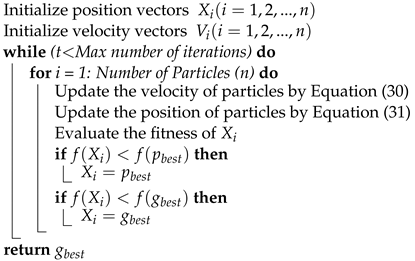
3.3.1. Particle Swarm Optimization

PSO is a population-based metaheuristic optimization algorithm developed in 1995 by Kennedy and Eberhart, inspired by the behavior of birds living in flocks in nature [46]. Generally, PSO is a population-based probability optimization method, which is preferred to produce solutions for multivariable and multiparameter optimization problems. It is frequently used in different optimization problems due to its high convergence speed and solutions. In adapting to various environmental conditions, such as avoiding predators or finding a rich food source, many animal swarms such as fish and birds communicate with each other, increasing their probability and speed of finding the real target. The essence of the PSO algorithm is a swarm and each particle is a part of it. In this swarm-based optimization algorithm, each particle consists of a position and velocity component, and an update is made in their positions by changing the velocity of the particles. Depending on the optimization problem, the updated positions of the particles are substituted in the objective function [46]. In the minimization process of the objective function, if the position value of the particle is smaller, than the best position value obtained, the new solution is kept in the memory in each iteration as shown in Algorithm 2. The position and velocity vectors of these particles are initially determined randomly, depending on the constraints. The velocities of randomly generated particles are computed as:
V i ( t + 1 ) = V i ( t ) + c 1 r a n d ( p b e s t X i ) + c 2 r a n d ( g b e s t X i )
in the next iteration, where X i , the position of i . particle, r a n d , is a uniformly random number between [0, 1]; p b e s t is the best position of the swarm; g b e s t is the best position within the group; and c 1 , c 2 are two constants which determine the weights of p b e s t and g b e s t , respectively. The position of the particles is obtained by adding the expression of velocity V i ( t + 1 ) to the current position X i as:
X i ( t + 1 ) = X i ( t ) + V i ( t + 1 )
In this optimization process, the position of each particle in the population is updated by changing the velocity vector. This update process consists of both the experimental knowledge of the particle and the knowledge it has socially acquired from neighboring particles.
Algorithm 2: Pseudo-code of PSO algorithm.
Electronics 11 01208 i002

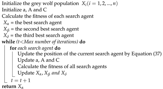
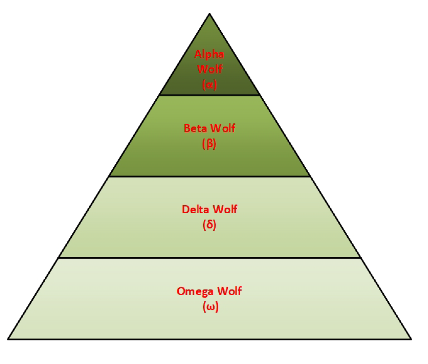
3.3.2. Grey Wolf Optimization

The GWO algorithm, inspired by the hunting hierarchy of grey wolves that live as a swarm in nature, is proposed by Mirjalili et al. [24]. As illustrated in Figure 3, the alpha wolf makes all hunting decisions in the herd, leads the swarm, and is located at the top of hunting pyramid. According to the order of social hierarchy in the herd, the top three wolves are alpha, beta, and omega, respectively. The candidate solutions are randomly generated in optimization process as with other metaheuristic optimization algorithms as shown in Algorithm 3. Among these candidate solutions, the best, the second, and the third candidate solution refers to to alpha ( X α ) , beta ( X β ) , and delta ( X δ ) positions, respectively. The other low candidate solution refers to the omega ( ω ) position. The hunting mechanism of grey wolves consists of following the prey and approaching, encircling, and attacking the prey. In the grey wolf optimization algorithm, the process of encircling the prey is carried out:
D = | C X p ( t ) X ( t ) |
X ( t + 1 ) = X p ( t ) A D
where t specifies the current iteration, A and C are constant vectors, X p is the position vector of the prey, and X defines the position vector of a grey wolf. A and D are calculated by:
A = 2 a r 1 a
C = 2 r 2
where a is linearly decreased from 2 to 0 over the course of the iterations, and r 1 and r 2 are random values generated between 0 and 1. The hunting process of grey wolves is expressed as:
D α = | C 1 X α X | D β = | C 2 X β X | D δ = | C 3 X δ X |
X 1 = X α A 1 D α X 2 = X β A 2 D β X 3 = X δ A 3 D δ
X ( t + 1 ) = X 1 + X 2 + X 3 3
where the positions of the best three agents are indicated by X α , X β , X δ ; the distance vectors ( D α , D β , D δ ) of candidate solutions are calculated according to the best three solutions; ( X 1 , X 2 , X 3 ) are the updated positions of the search agents; and X ( t + 1 ) is the next iteration position.
Algorithm 3: Pseudo-code of GWO algorithm.
Electronics 11 01208 i003

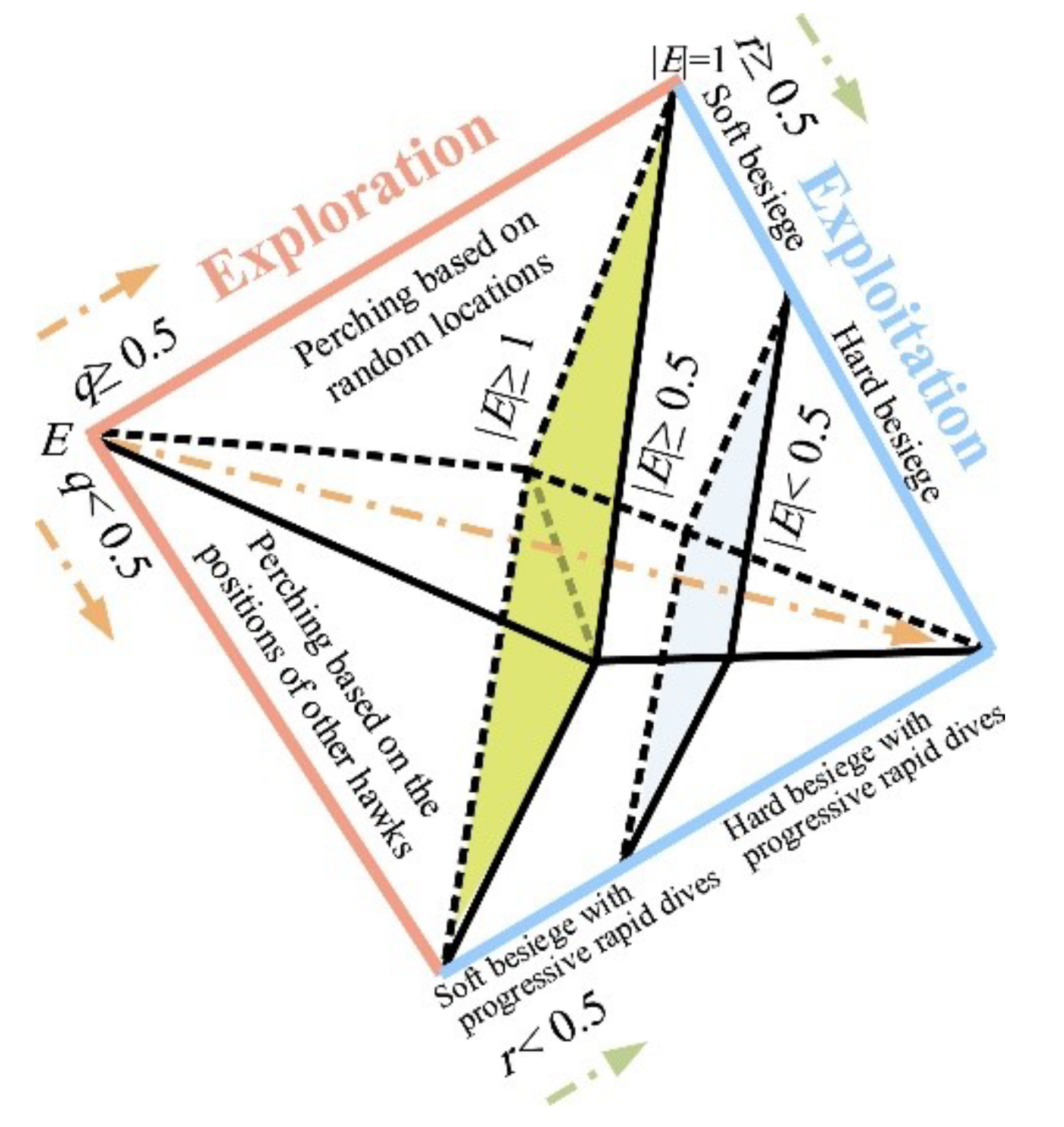
3.3.3. Harris Hawk Optimization

In this section, the exploration, transition from exploration to exploitation, and exploitation phases of the HHO component of the hybrid GWO–HHO algorithm proposed in the study are explained. In this algorithm, the hunting strategy of Harris hawks, one of the smart birds in nature, is imitated. Harris hawks act as a swarm, especially during the rabbit-hunting process. Each swarm has a leader. The leader and other members of the swarm primarily make exploration flights. After the prey is detected, the hunting process begins. HHO is gradient-free optimization method; hence, it can be applied to many nonlinear engineering problems depending on a suitable formulation [45]. Harris hawks’ main tactic in hunting is called the “surprise attack”. In this clever strategy, several hawks collaboratively try to attack from different directions and simultaneously approach the prey that has been found to have fled outside the shelter. The attack can be completed quickly, with the hawks catching their prey in a matter of seconds. All phases of the HHO’s exploration and exploitation processes are shown in Figure 4.
  • Exploration phase: Although Harris hawks have strong eyes, sometimes they may not be able to detect their prey easily. In this situation, Harris hawks often wait in the desert area and observe their surroundings. This process continues in a loop. Harris hawks in each loop are identified as candidate solutions. The hawk, who is in the best position in relation to the rabbit in the loop, represents the optimum solution. The HHO algorithm uses two different strategies in the hunt search process. These strategies can be described by [45]:
    X ( t + 1 ) = X r a n d ( t ) r 1 | X r a n d 2 r 2 X ( t ) | q 0.5 ( X r a b b i t ( t ) X m ( t ) ) r 3 ( L B + r 4 ( U B L B ) ) q < 0.5
    where X ( t + 1 ) represents the position of Harris hawks in the next iteration t ; X ( t ) denotes the current position of Harris hawks; X r a b b i t indicates the position of the rabbit; X m ( t ) is the average position of the current population of Harris Hawks; X r a n d ( t ) represents a randomly selected Harris hawk from the current population; r 1 , r 2 , r 3 , r 4 , and q are random numbers between [ 0 , 1 ] ; and U B and L B show the upper and lower bounds of the variables, respectively. The average position of hawks is determined by:
    X m ( t ) = 1 N i = 1 N X i ( t )
    where N represents the total number of Harris hawks, and X i ( t ) indicates the location of each Harris hawk in iteration t.
  • Transition from exploration to exploitation phase: Harris hawks begin the exploitation phase by developing different attack models according to the energy of the prey after the exploration process is completed. This process is modelled in [45] as:
    E = 2 E 0 ( 1 t T )
    where E 0 is the initial energy value of the prey randomly defined in the range of [ 0 , 1 ] , E is the energy of the escaping prey, and T is the maximum number of iterations.
  • Exploitation phase: At this phase, the Harris hawk attacks its prey and makes the surprise attack move. In response to this situation, the prey tries to escape. In this case, the Harris hawk basically develops four different strategies. The energy of the prey and the chance of catching the escaping prey are indicated by E and r, respectively:
    Soft besiege ( r 0.5 and | E | 0.5 )
    In this strategy, the Harris hawk makes misleading jumps at its prey and tries to reduce the energy of its prey. This soft besiege strategy is mathematically described by:
    X ( t + 1 ) = Δ X ( t ) E | J X r a b b i t ( t ) X ( t ) |
    Δ X ( t ) = X r a b b i t ( t ) X ( t )
    where Δ X ( t ) is the difference between the current position in the t-th iteration and the current position of the prey, and J is a value that changes with each iteration to simulate the natural motion of the prey.
    Hard besiege ( r 0.5 and | E | < 0.5 )
    In this strategy, the energy of the prey is very low. The hawk hardly makes any besiege to throw his surprise claws on its prey. This strategy can be mathematically modeled as:
    X ( t + 1 ) = X r a b b i t ( t ) E | Δ X ( t ) |
    where X r a b b i t ( t ) represents the current position of prey, Δ X ( t ) is the difference between the current position in the t-th iteration and the current position of the prey.
    Soft besiege with progressive rapid dives ( r < 0.5 and | E | 0.5 )
    In this strategy, the prey has enough energy to escape. The Harris hawk is still performing the soft besiege strategy before the surprise jump. This process is smarter than the previous strategy. Before the hawks start their soft besiege, they decide their next move based on the following calculation:
    Y = X r a b b i t ( t ) E | J X r a b b i t ( t ) X ( t ) |
    where X r a b b i t ( t ) indicates the current position of the prey, and J is a value that changes with each iteration to simulate the natural motion of the prey. This situation is compared with the previous dive to decide whether such a move would be a good dive. If the situation is unfavorable, the hawks dive into their prey suddenly. When deciding on this, a Levy-flight-based movement structure is used. This situation is defined by:
    Z = Y + S × L F ( D )
    where Z is the variable that decides whether the hawk will make a move on its prey, Y indicates its position in relation to the decreasing energy of the prey, D is the size of the problem, S is a random vector of size 1 x D , and  L F is the Levy flight function and is defined by:
    L F ( x ) = 0.01 u × σ | v | 1 β σ = Γ ( 1 + β ) × s i n ( π β 2 ) Γ ( 1 + β 2 ) × β × 2 ( β 1 2 ) 1 β
    where u and v are the random numbers between (0, 1), and β is 1.5. Note that the Levy flight algorithm is added to the exploitation phase to ensure that the local search process can be continued without becoming stuck at local optimum points. The positions of the hawks in the soft besiege phase are updated by:
    X ( t + 1 ) = Y if F ( Y ) < F ( X ( t ) ) Z if F ( Z ) < F ( X ( t ) )
    where Y and Z are obtained using Equations (40) and (41).
    Hard besiege with progressive rapid dives ( r < 0.5 and | E | < 0.5 ) In this strategy, the prey does not have enough energy to escape. The Harris hawk makes a fierce siege before its surprise jump to catch its prey. The hard besiege situation is expressed by:
    X ( t + 1 ) = Y if F ( Y ) < F ( X ( t ) ) Z if F ( Z ) < F ( X ( t ) )
    where Y and Z are defined as:
    Y = X r a b b i t ( t ) E | J X r a b b i t ( t ) X m ( t ) |
    Z = Y + S × L F ( D )

3.3.4. The Proposed Optimization Algorithm

In this study, a hybrid HHO–GWO algorithm is proposed by combining the HHO algorithm with its random search capability and high convergence speed and the GWO algorithm, which has a high performance in avoiding local optima, so that the quadcopter can both avoid obstacles and track the planned path with minimum error. This algorithm ensures the robustness of the controller, even with sudden mass changes in the quadcopter during payload hold and release. The pseudo-code of the proposed algorithm for this study is presented in Algorithm 4.
Algorithm 4: Pseudo-code of hybrid HHO–GWO algorithm
Electronics 11 01208 i004

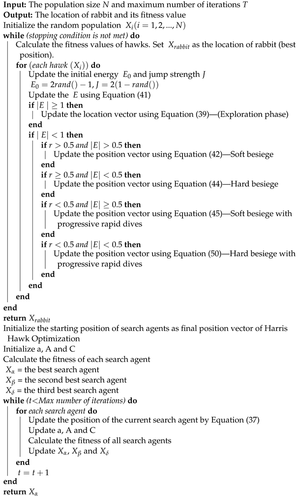
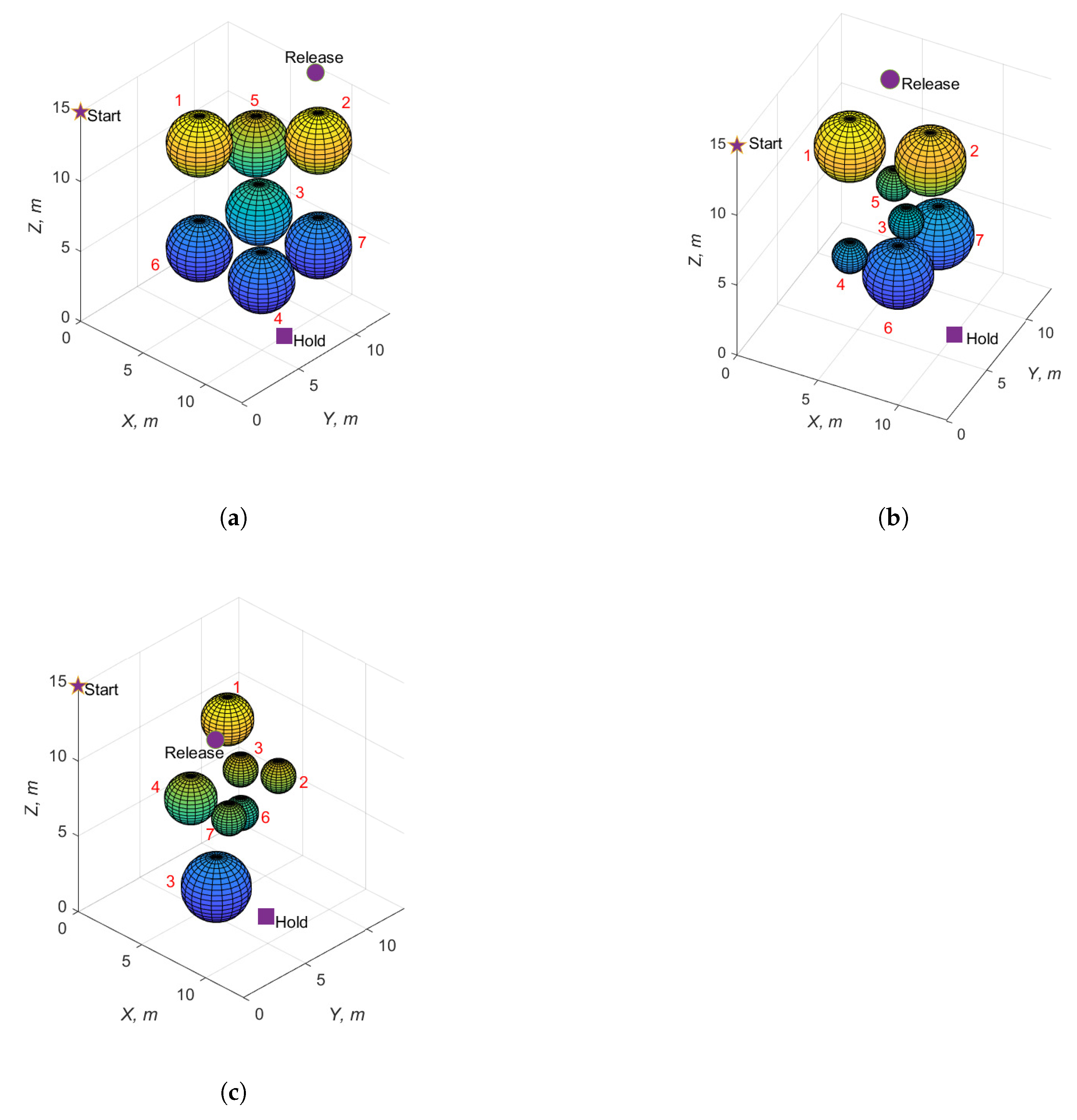
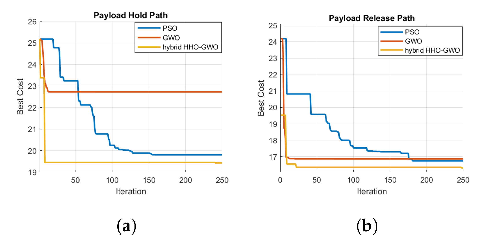
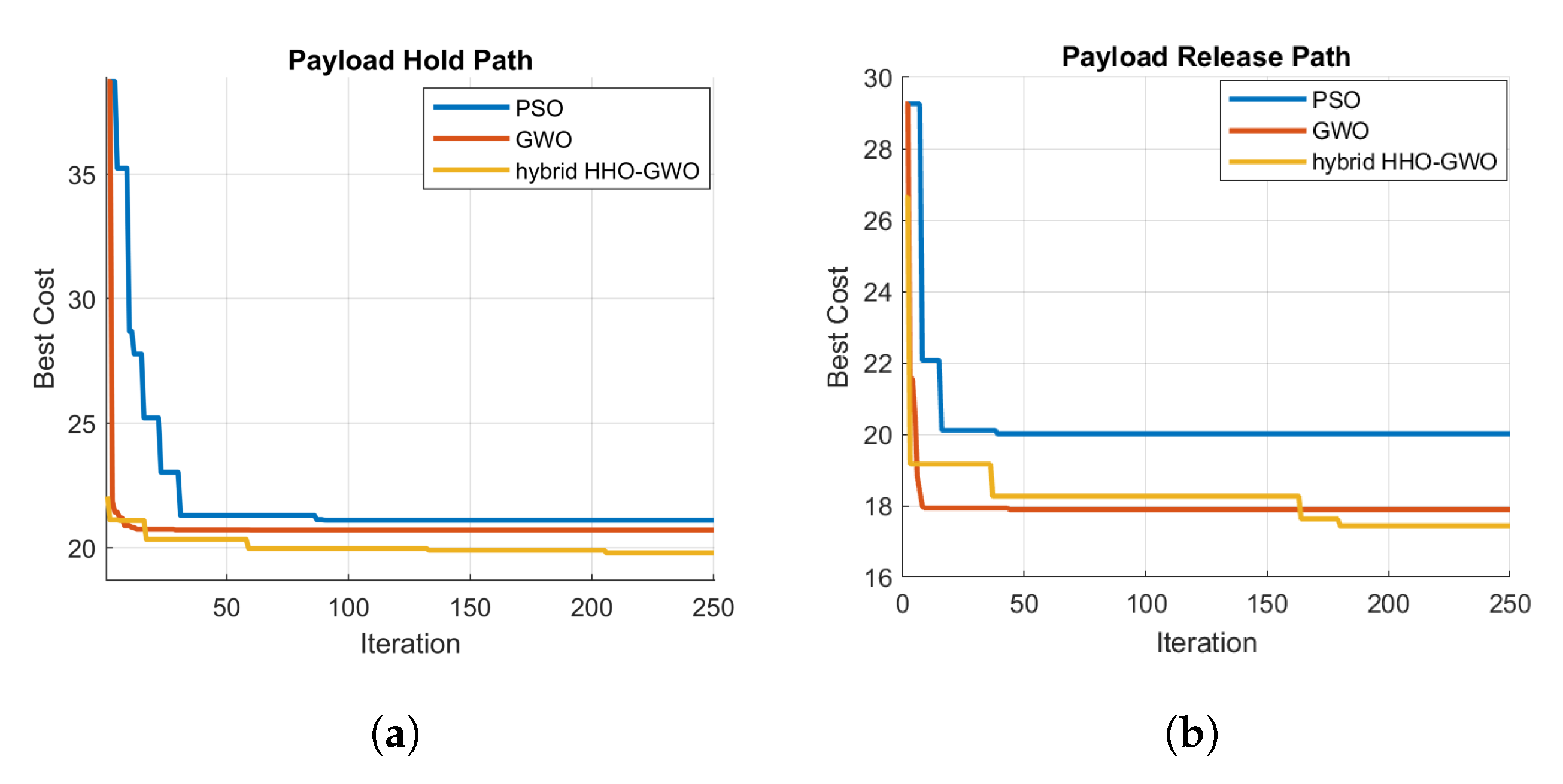
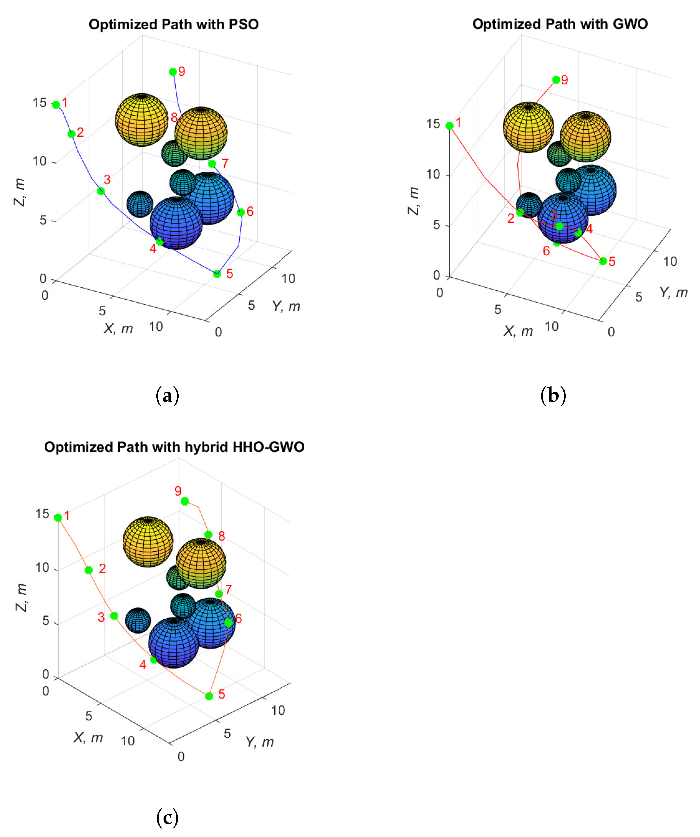
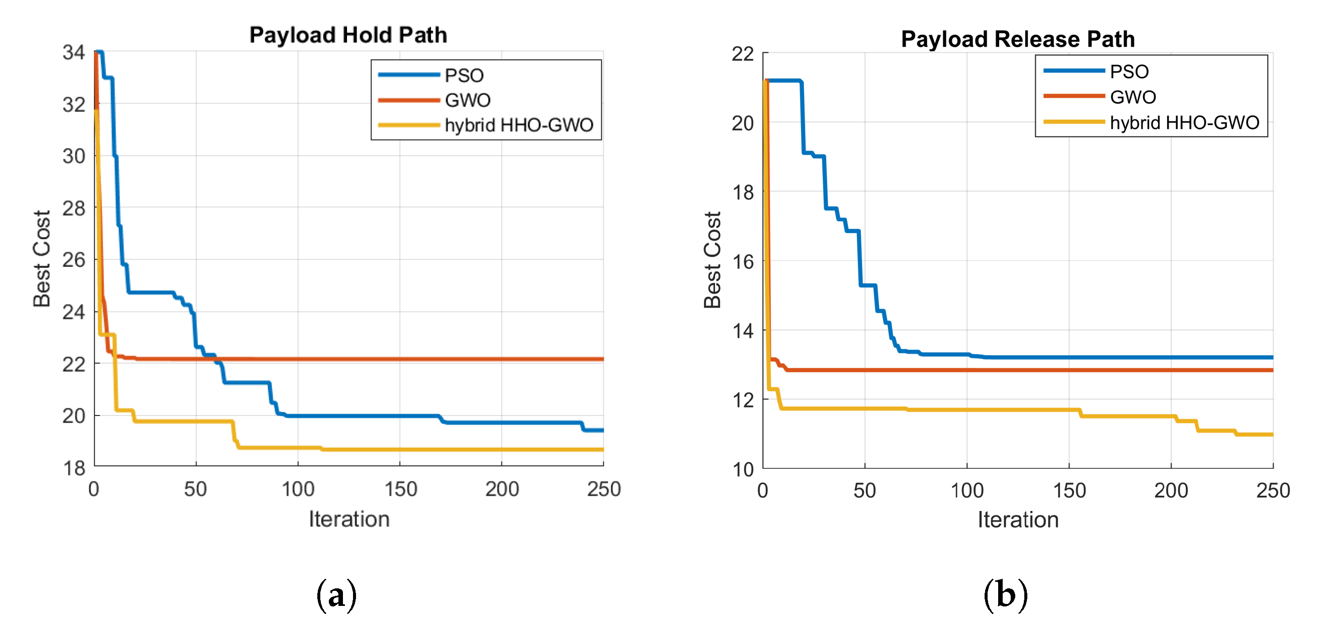
4. Payload Hold-Release Mission Planning

In this study, a path planning and tracking algorithm is proposed on three different maps. In order to guarantee that the algorithms run do not memorize the path, three maps with different starting and ending points, containing obstacles at different locations, are generated. On the first map, there are obstacles of equal size with a radius of 2 m. On the second map, there are obstacles of two different sizes with radii of 1 m and 2 m. On the third map, there are obstacles in three different sizes with radii of 1 m, 1.5 m, and 2 m. The environmental difficulty level of Map 1, Map 2, and Map 3 range from weak to strong, respectively, in performing the payload hold-and-release mission by coping with obstacles. Seven separate spherical obstacles are placed on each of the maps. The locations of these spherical barriers on three different maps are given in Table 1. As stated in the Table 1, the location of each obstacle in 3D space is expressed as the X, Y, Z positions and radius R. These spherical barriers are positioned in 3D space, as shown in Figure 5. Here, the point where the quadcopter starts its mission, holds and releases the payload is shown as star, square and circle, respectively. In addition, the numbers on the figure are used to label the obstacles. The numbers on the figure are used to name the obstacles. Considering the safe and shortest path conditions of the quadrotor on these generated maps, waypoints are determined by metaheuristic optimization algorithms such as PSO, GWO, and hybrid HHO–GWO. By following this determined path, the payload hold–release performance of the quadrotor has been analyzed.

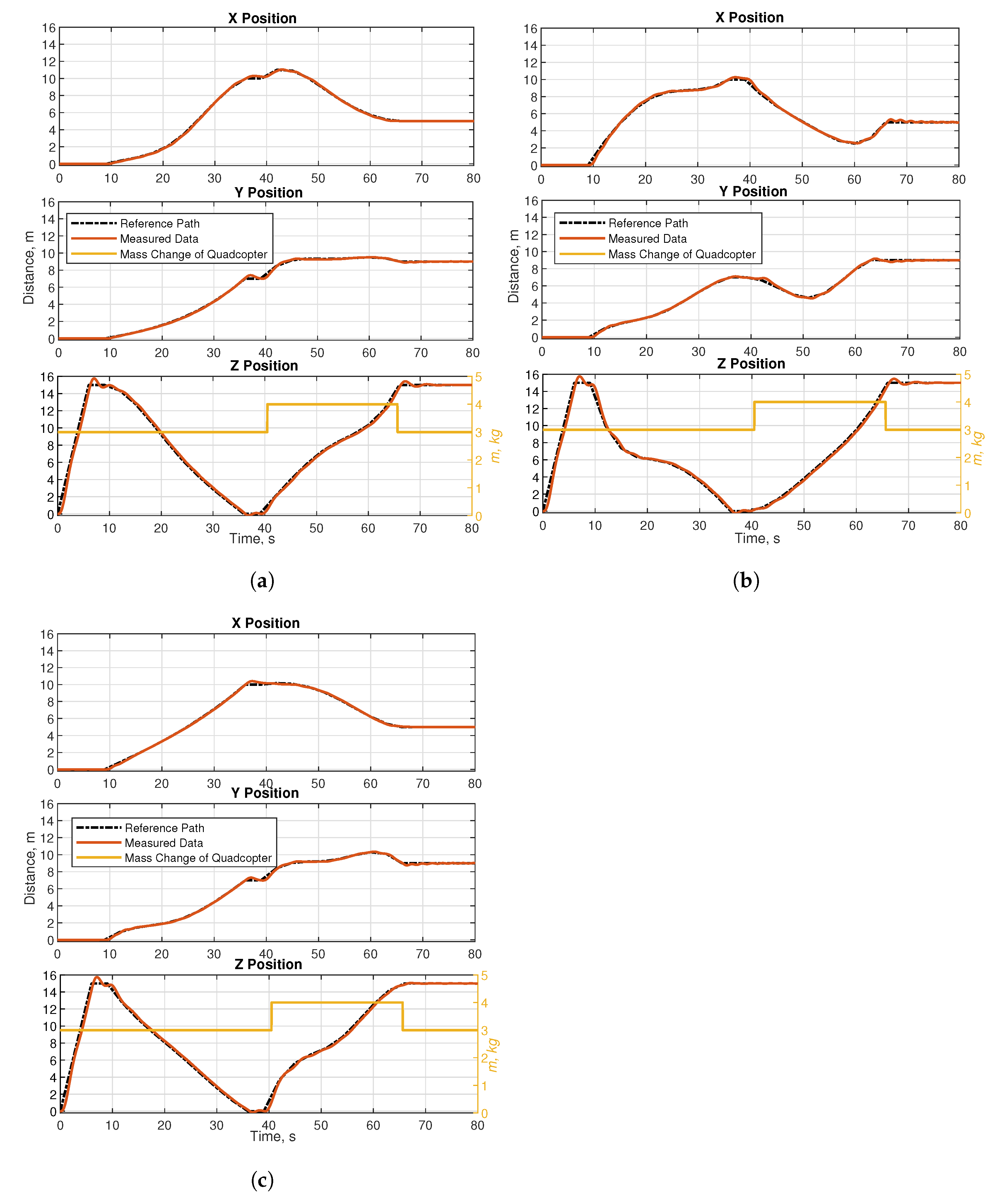
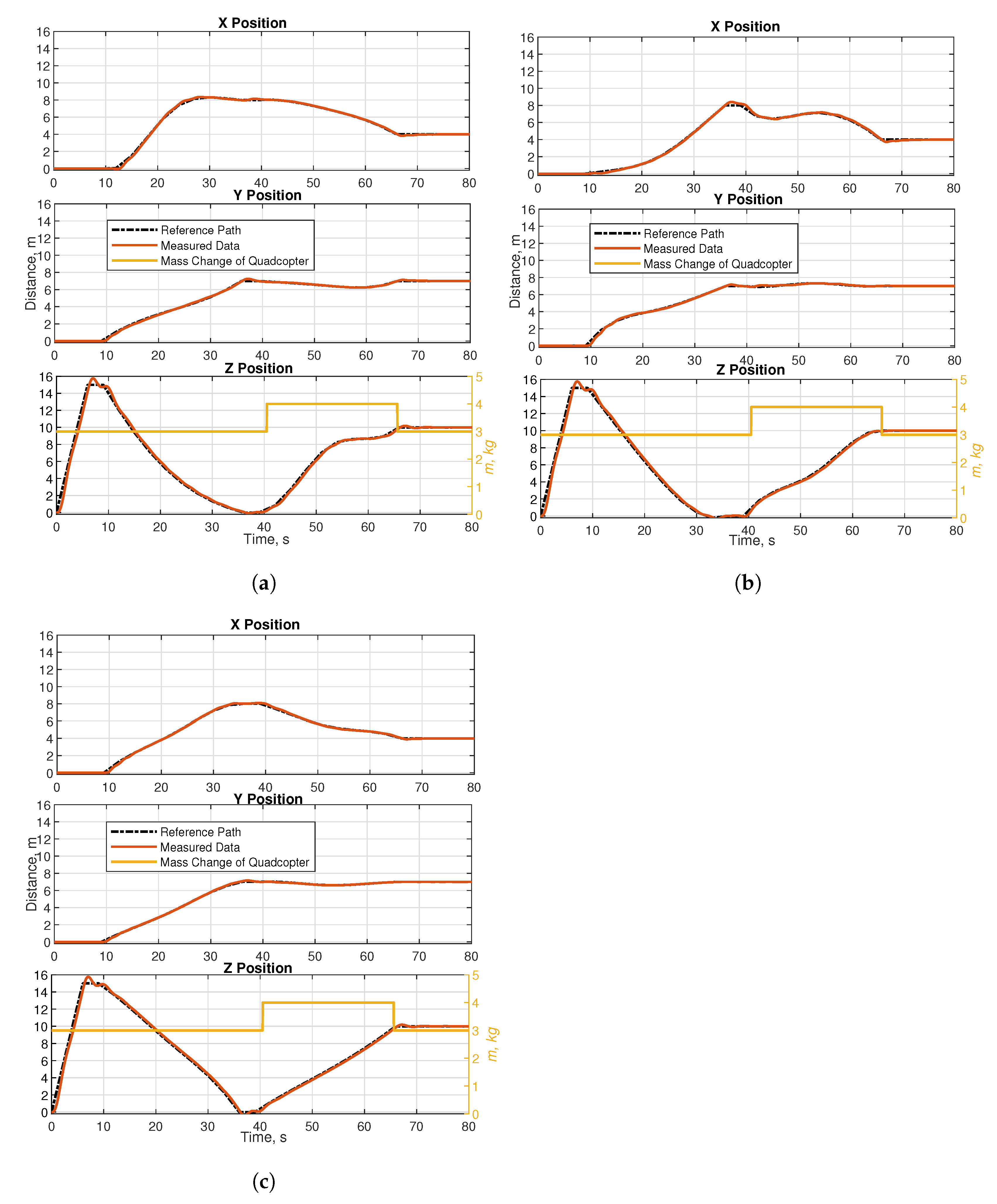
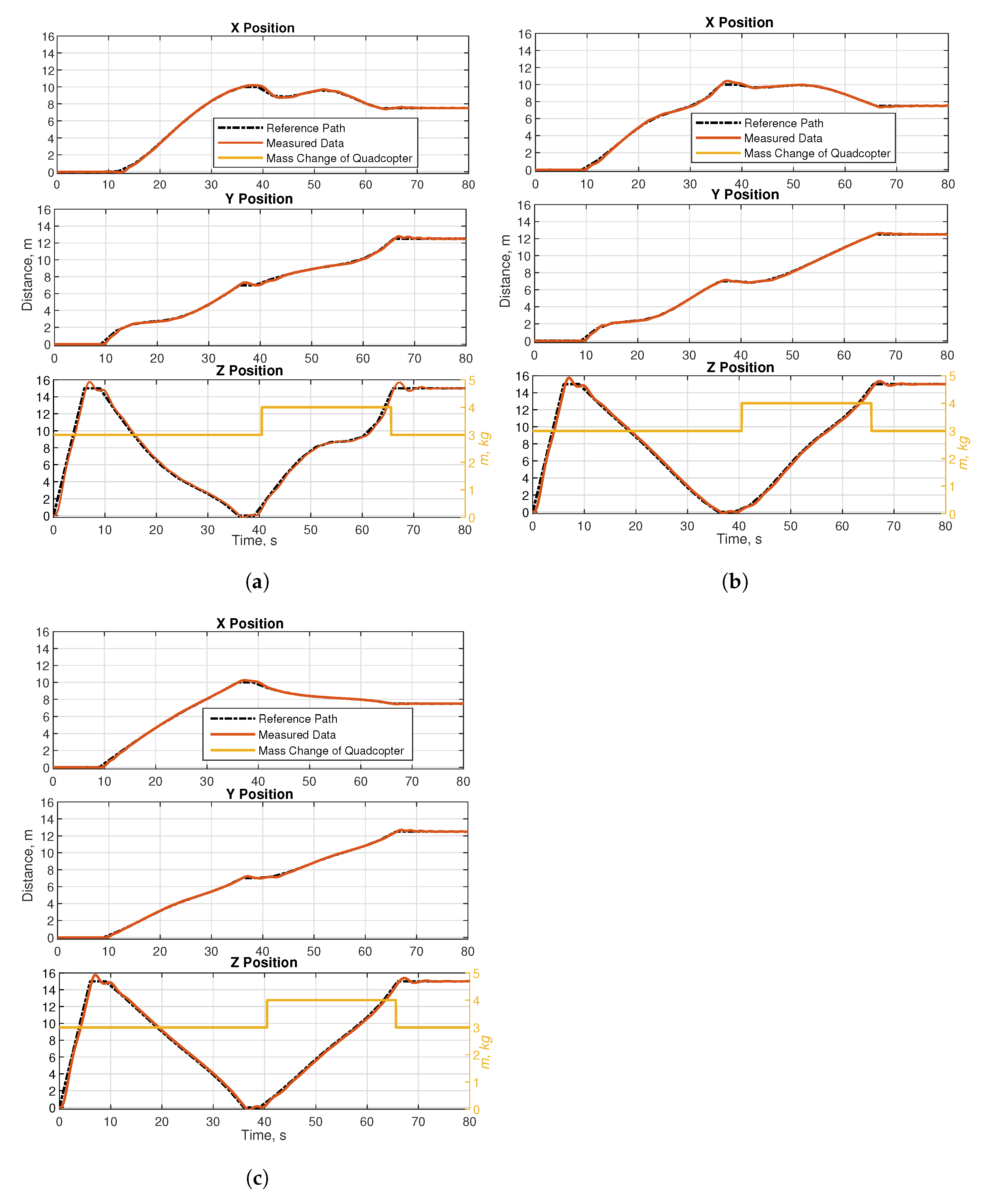
5. Experimental Results and Discussion

The performance comparison of the path planning and tracking control strategy is presented in this section. Firstly, the path planning performance of the quadcopter is examined on three different maps. Generating the shortest and safest path of quadcopter on all three maps is performed with the PSO, GWO, and hybrid HHO–GWO algorithms. The quadcopter at origin point (0, 0, 0) rises by 15 m along the Z-axis in all 3 maps. Afterwards, the payload holds the path from the first to the fifth waypoints, and the payload release path from the fifth to ninth waypoints are generated by metaheuristic optimization algorithms such as PSO, GWO, and hybrid HHO–GWO. The mass of payload is 1 kg. Therefore, the total mass of quadcopter has been changed from 3 kg to 4 kg in all missions. The root mean squared error (RMSE) performance criterion in path planning and tracking is denoted as:
R M S E = 1 N m i = 1 N m ( X r e f i X i ) 2 + ( Y r e f i Y i ) 2 + ( Z r e f i Z i ) 2
where X r e f i , Y r e f i , and Z r e f i are reference positions of the quadcopter; X i , Y i , and Z i are measured positions of the quadcopter in X, Y, and Z axes, respectively; and the total number of measurements is expressed with N m . The energy efficiency can be calculated as:
E e f f = E b E t E b × 100
where E b is the total energy of the battery, and E t is the total energy consumed by the quadcopter. The generated waypoints are presented for Scenario 1 in Table 2. The distances of the paths created are 37.53 m, 36.26 m, 35.68 m in Scenario 1 for the PSO, GWO, and hybrid HHO–GWO, respectively. The performance of the payload hold and release path is demonstrated in Figure 6. The path generated by metaheuristic optimization algorithms is illustrated on Scenario 1 with obstacles in Figure 7. When the convergence rate and minimum point are investigated, the maximum convergence rate and minimum point has been obtained for the proposed hybrid HHO–GWO algorithm. The shortest distance path is obtained with the hybrid HHO–GWO on Scenario 1.
The generated waypoints are introduced for Scenario 2 in Table 3. The distances of the paths created are 37.47 m, 40.72 m, and 36.73 m in Scenario 2 for the PSO, GWO, and hybrid HHO–GWO, respectively. The performance of the payload hold-and-release path is displayed in Figure 8. The paths generated by the metaheuristic optimization algorithms are indicated in Scenario 2 with obstacles in Figure 9. When the convergence rate and minimum point are investigated, the maximum convergence rate and minimum point has been obtained for the proposed hybrid HHO–GWO algorithm. The generated minimum path distance is obtained for the hybrid HHO–GWO in Scenario 2.
The generated waypoints are demonstrated for Scenario 3 in Table 4. The distances of the paths created are 31.32 m, 32.24 m, and 29.59 m on Map 3 for the PSO, GWO, and hybrid HHO–GWO, respectively. The performance of the payload hold-and-release path is displayed in Figure 10. The paths generated by the metaheuristic optimization algorithms are shown in Scenario 3 with obstacles in Figure 11. The numbers on Figure 7, Figure 9 and Figure 11 are used to label the waypoints obtained by the optimization algorithms. When the convergence rate and minimum point are investigated, the maximum convergence rate and minimum point were obtained for the proposed hybrid HHO–GWO algorithm. The generated minimum path distance is obtained for hybrid HHO–GWO in Scenario 3. To summarize, the path planning on all three maps is obtained for the proposed hybrid HHO–GWO algorithm for minimum distance and the maximum converge rate. The PSO algorithm is run 500 times for Scenarios 1–3, and the average running times for each scenario are determined as 66.14 s, 66.16 s, and 66.01 s, respectively. The GWO algorithm is run 500 times for Scenarios 1–3, and the average running times for each scenario are 65.12 s, 65.25 s, and 65.11 s, respectively. The proposed hybrid HHO–GWO algorithm is run 500 times for Scenarios 1–3, and the average running times for each scenario are measured as 64.09 s, 64.68 s, and 64.71 s, respectively. Note that all algorithms mentioned in the study are run on a PC device, which has an Intel i7-10750H, 6 cores, 2.6 GHz Turbo, and 32 GB RAM. All codes are compiled with MATLAB 2020b.
The path tracking performance of the quadcopter is analyzed with these generated waypoints. The payload hold and release are carried out in waypoints 5 and 9, respectively. The performance of the quadcopter under both path tracking and sudden payload change is examined. The path tracking in a payload hold–release mission is illustrated in Figure 12, Figure 13 and Figure 14 for Scenarios 1, 2, and 3, respectively. The total path, RMSE, target time, and energy efficiency performance criteria of metaheuristic algorithms are presented in Table 5. The total measured paths are 53.025 m, 51.631 m, and 50.7 m, and the mean square errors are 21.76 m, 19.98 m, and 19.57 m for PSO, GWO, and hybrid HHO–GWO, respectively, in Scenario 1. The total times of the payload hold–release mission in Scenario 1 are 66.15 s, 65.01 s, and 64.12 s for the PSO, GWO, and hybrid HHO–GWO, respectively. The energy efficiencies of the quadcopter in Scenario 1 are obtained as 64.51%, 67.42%, and 68.08% for the PSO, GWO, and hybrid HHO–GWO respectively. The total measured paths are 52.92 m, 56.52 m, and 52.51 m, and the mean square errors are 19.86 m, 22.7 m, and 19.35 m for the PSO, GWO, and hybrid HHO–GWO, respectively, in Scenario 2. The total mission times are 66.18 s, 65.24 s, and 64.76 s, and the energy efficiencies obtained are 67.92%, 63.33%, and 68.74% for the PSO, GWO, and hybrid HHO–GWO, respectively, in Scenario 2. The total measured paths are 46.87 m, 47.80 m, and 44.72 m, and the mean square errors are 17.65 m, 18.49 m, and 16.92 m for the PSO, GWO, and hybrid HHO–GWO, respectively, in Scenario 3. The total mission times are 65.99 s, 65.01 s, and 64.71 s, and the energy efficiencies are 66.74%, 65.5%, and 68.81% for the PSO, GWO, and hybrid HHO–GWO, respectively, in Scenario 3. The minimum total path, mean square error, target time, and energy efficiency are obtained for the hybrid HHO–GWO in all Scenarios. When the path tracking performance of the quadcopter in Figure 14 for Scenario 3, which has the highest environmental difficulty level, is evaluated, it is seen that the least change in the Z-axis occurs with the proposed algorithm. This shows that the energy is used optimally. The results show that the hybrid HHO–GWO algorithm has the highest energy efficiency.
To summarize, the path planning and tracking control strategy of the quadcopter have been proposed in this study. The path planning has been achieved via PSO, GWO, and the proposed hybrid HHO–GWO algorithms. The results of path planning show that the shortest and safest paths are obtained for all scenarios. After this, the path-tracking performance of the quadcopter in a payload hold–release mission is investigated for all scenarios. The path-tracking results express that the minimum total path, mean square error, target time and energy efficiency of quadcopter in payload transportation mission have been obtained for all scenarios. The path-tracking error due to the mass uncertainty of the quadcopter has been minimized in all scenarios with obstacles. The contributions of this study are the following:
  • A hybrid HHO–GWO optimization algorithm with high convergence speed for path planning has been proposed,
  • The position error of the quadcopter caused by the sudden change during payload holding and releasing is examined;
  • The errors that occur in path tracking under sudden payload changes are minimized with the newly proposed control strategy.

6. Conclusions and Future Work

In this study, a new metaheuristic path planning and tracking algorithm for payload hold–release mission is proposed to avoid obstacles. A hybrid HHO–GWO algorithm is proposed by combining the HHO algorithm, with high convergence speed, and the GWO algorithm, which has a high performance in avoiding local optima, so that the quadcopter can both avoid obstacles and track the planned path with minimum error. The performance of the proposed path-planning algorithm is compared with PSO and GWO. The minimum path distance and maximum convergence rate have been obtained with the newly proposed hybrid HHO–GWO metaheuristic optimization algorithm. The waypoints that the quadcopter desires to track are generated with the optimization algorithm not only minimizing distance but also energy. The path tracking has been carried out by these generated waypoints. The payload hold-and-release mission has been realized with a path-tracking controller. The mass component in the quadcopter model is changed during payload holding and releasing. The position errors occur in path tracking with the sudden mass change of the quadcopter in this payload holding and releasing task. The results of path tracking are indicated by the minimum total path, mean square error, total time and consumed energy have been obtained for the newly proposed hybrid HHO–GWO. The most important contribution of this study is that the proposed control strategy and the position error caused by this mass uncertainty can be minimized. It is planned to perform environmental tests of the proposed metaheuristic-based approach by embedding it on a single UAV in the future. By comparing the results obtained with the results of our current study, studies will be focused on the optimum solution of path generation and tracking problems with the cooperation of multiple UAVs.

Author Contributions

Conceptualization, E.B., A.A. and R.H.; methodology, E.B., A.A. and R.H.; software, E.B., A.A. and R.H.; writing—original draft preparation, E.B. and A.A.; writing—review and editing, E.B., A.A. and R.H. All authors have read and agreed to the published version of the manuscript.

Funding

This research received no external funding.

Conflicts of Interest

The authors declare no conflict of interest.

References

  1. Yu, X.; Li, C.; Zhou, J. A constrained differential evolution algorithm to solve UAV path planning in disaster scenarios. Knowl.-Based Syst. 2020, 204, 106209. [Google Scholar] [CrossRef]
  2. Ropero, F.; Muñoz, P.; R-Moreno, M.D. TERRA: A path planning algorithm for cooperative UGV–UAV exploration. Eng. Appl. Artif. Intell. 2019, 78, 260–272. [Google Scholar] [CrossRef]
  3. Sivčev, S.; Rossi, M.; Coleman, J.; Omerdić, E.; Dooly, G.; Toal, D. Collision detection for underwater ROV manipulator systems. Sensors 2018, 18, 1117. [Google Scholar] [CrossRef] [PubMed] [Green Version]
  4. De Vivo, F.; Battipede, M.; Johnson, E. Infra-red line camera data-driven edge detector in UAV forest fire monitoring. Aerosp. Sci. Technol. 2021, 111, 106574. [Google Scholar] [CrossRef]
  5. Altan, A.; Hacıoğlu, R. Model predictive control of three-axis gimbal system mounted on UAV for real-time target tracking under external disturbances. Mech. Syst. Signal Process. 2020, 138, 106548. [Google Scholar] [CrossRef]
  6. Silvagni, M.; Tonoli, A.; Zenerino, E.; Chiaberge, M. Multipurpose UAV for search and rescue operations in mountain avalanche events. Geomat. Nat. Hazards Risk 2017, 8, 18–33. [Google Scholar] [CrossRef] [Green Version]
  7. Cui, L.; Zhang, R.; Yang, H.; Zuo, Z. Adaptive super-twisting trajectory tracking control for an unmanned aerial vehicle under gust winds. Aerosp. Sci. Technol. 2021, 115, 106833. [Google Scholar] [CrossRef]
  8. Causa, F.; Fasano, G. Multiple UAVs trajectory generation and waypoint assignment in urban environment based on DOP maps. Aerosp. Sci. Technol. 2021, 110, 106507. [Google Scholar] [CrossRef]
  9. Sun, P.; Boukerche, A. Performance modeling and analysis of a UAV path planning and target detection in a UAV-based wireless sensor network. Comput. Netw. 2018, 146, 217–231. [Google Scholar] [CrossRef]
  10. Zhang, Z.; Li, J.; Wang, J. Sequential convex programming for nonlinear optimal control problems in UAV path planning. Aerosp. Sci. Technol. 2018, 76, 280–290. [Google Scholar] [CrossRef]
  11. Huang, Y.; Mei, W.; Xu, J.; Qiu, L.; Zhang, R. Cognitive UAV communication via joint maneuver and power control. IEEE Trans. Commun. 2019, 67, 7872–7888. [Google Scholar] [CrossRef] [Green Version]
  12. Zhang, Y.; Zhang, R.; Li, H. Graph-based path decision modeling for hypersonic vehicles with no-fly zone constraints. Aerosp. Sci. Technol. 2021, 116, 106857. [Google Scholar] [CrossRef]
  13. Radmanesh, R.; Kumar, M.; French, D.; Casbeer, D. Towards a PDE-based large-scale decentralized solution for path planning of UAVs in shared airspace. Aerosp. Sci. Technol. 2020, 105, 105965. [Google Scholar] [CrossRef]
  14. Pehlivanoglu, Y.V. A new vibrational genetic algorithm enhanced with a Voronoi diagram for path planning of autonomous UAV. Aerosp. Sci. Technol. 2012, 16, 47–55. [Google Scholar] [CrossRef]
  15. Baumann, M.; Leonard, S.; Croft, E.A.; Little, J.J. Path planning for improved visibility using a probabilistic road map. IEEE Trans. Robot. 2010, 26, 195–200. [Google Scholar] [CrossRef]
  16. Bayili, S.; Polat, F. Limited-Damage A*: A path search algorithm that considers damage as a feasibility criterion. Knowl.-Based Syst. 2011, 24, 501–512. [Google Scholar] [CrossRef]
  17. Moon, C.B.; Chung, W. Kinodynamic planner dual-tree RRT (DT-RRT) for two-wheeled mobile robots using the rapidly exploring random tree. IEEE Trans. Ind. Electron. 2014, 62, 1080–1090. [Google Scholar] [CrossRef]
  18. Battulwar, R.; Winkelmaier, G.; Valencia, J.; Naghadehi, M.Z.; Peik, B.; Abbasi, B.; Parvin, B.; Sattarvand, J. A Practical Methodology for Generating High-Resolution 3D Models of Open-Pit Slopes Using UAVs: Flight Path Planning and Optimization. Remote. Sens. 2020, 12, 2283. [Google Scholar] [CrossRef]
  19. Huang, L.; Qu, H.; Ji, P.; Liu, X.; Fan, Z. A novel coordinated path planning method using k-degree smoothing for multi-UAVs. Appl. Soft Comput. 2016, 48, 182–192. [Google Scholar] [CrossRef] [Green Version]
  20. Dorigo, M.; Birattari, M.; Stutzle, T. Ant colony optimization. IEEE Comput. Intell. Mag. 2006, 1, 28–39. [Google Scholar] [CrossRef]
  21. Ali, Z.A.; Zhangang, H.; Hang, W.B. Cooperative path planning of multiple UAVs by using max–min ant colony optimization along with cauchy mutant operator. Fluct. Noise Lett. 2021, 20, 2150002. [Google Scholar] [CrossRef]
  22. Shao, S.; Peng, Y.; He, C.; Du, Y. Efficient path planning for UAV formation via comprehensively improved particle swarm optimization. ISA Trans. 2020, 97, 415–430. [Google Scholar] [CrossRef] [PubMed]
  23. Dewangan, R.K.; Shukla, A.; Godfrey, W.W. Three dimensional path planning using grey wolf optimizer for UAVs. Appl. Intell. 2019, 49, 2201–2217. [Google Scholar] [CrossRef]
  24. Mirjalili, S.; Mirjalili, S.M.; Lewis, A. Grey wolf optimizer. Adv. Eng. Softw. 2014, 69, 46–61. [Google Scholar] [CrossRef] [Green Version]
  25. Ganguly, S. Multi-objective distributed generation penetration planning with load model using particle swarm optimization. Decis. Mak. Appl. Manag. Eng. 2020, 3, 30–42. [Google Scholar] [CrossRef]
  26. Negi, G.; Kumar, A.; Pant, S.; Ram, M. Optimization of complex system reliability using hybrid grey wolf optimizer. Decis. Mak. Appl. Manag. Eng. 2021, 4, 241–256. [Google Scholar] [CrossRef]
  27. Das, M.; Roy, A.; Maity, S.; Kar, S.; Sengupta, S. Solving fuzzy dynamic ship routing and scheduling problem through new genetic algorithm. Decis. Mak. Appl. Manag. Eng. 2021. [Google Scholar] [CrossRef]
  28. Sasongko, R.A.; Rawikara, S.; Tampubolon, H.J. UAV obstacle avoidance algorithm based on ellipsoid geometry. J. Intell. Robot. Syst. 2017, 88, 567–581. [Google Scholar] [CrossRef]
  29. Singla, A.; Padakandla, S.; Bhatnagar, S. Memory-based deep reinforcement learning for obstacle avoidance in UAV with limited environment knowledge. IEEE Trans. Intell. Transp. Syst. 2019, 22, 107–118. [Google Scholar] [CrossRef]
  30. Iacono, M.; Sgorbissa, A. Path following and obstacle avoidance for an autonomous UAV using a depth camera. Robot. Auton. Syst. 2018, 106, 38–46. [Google Scholar] [CrossRef]
  31. Zheng, L.; Zhang, P.; Tan, J.; Li, F. The obstacle detection method of UAV based on 2D LIDAR. IEEE Access 2019, 7, 163437–163448. [Google Scholar] [CrossRef]
  32. Liu, Y.; Rajappa, S.; Montenbruck, J.M.; Stegagno, P.; Bülthoff, H.; Allgöwer, F.; Zell, A. Robust nonlinear control approach to nontrivial maneuvers and obstacle avoidance for quadrotor UAV under disturbances. Robot. Auton. Syst. 2017, 98, 317–332. [Google Scholar] [CrossRef]
  33. Altan, A.; Aslan, Ö.; Hacıoğlu, R. Real-time control based on NARX neural network of hexarotor UAV with load transporting system for path tracking. In Proceedings of the 2018 6th International Conference on Control Engineering & Information Technology (CEIT), Istanbul, Turkey, 25–27 October 2018; pp. 1–6. [Google Scholar]
  34. Shirani, B.; Najafi, M.; Izadi, I. Cooperative load transportation using multiple UAVs. Aerosp. Sci. Technol. 2019, 84, 158–169. [Google Scholar] [CrossRef]
  35. Lee, H.I.; Yoo, D.W.; Lee, B.Y.; Moon, G.H.; Lee, D.Y.; Tahk, M.J.; Shin, H.S. Parameter-robust linear quadratic Gaussian technique for multi-agent slung load transportation. Aerosp. Sci. Technol. 2017, 71, 119–127. [Google Scholar] [CrossRef] [Green Version]
  36. Hashemi, D.; Heidari, H. Trajectory planning of quadrotor UAV with maximum payload and minimum oscillation of suspended load using optimal control. J. Intell. Robot. Syst. 2020, 100, 1369–1381. [Google Scholar] [CrossRef]
  37. Kuantama, E.; Vesselenyi, T.; Dzitac, S.; Tarca, R. PID and Fuzzy-PID control model for quadcopter attitude with disturbance parameter. Int. J. Comput. Commun. Control. 2017, 12, 519–532. [Google Scholar] [CrossRef] [Green Version]
  38. Selby, W.C. Autonomous Navigation and Tracking of Dynamic Surface Targets On-Board a Computationally Impoverished Aerial Vehicle. Ph.D. Thesis, Massachusetts Institute of Technology, Cambridge, MA, USA, 2011. [Google Scholar]
  39. Luukkonen, T. Modelling and control of quadcopter. Indep. Res. Proj. Appl. Math. Espoo 2011, 22, 22. [Google Scholar]
  40. Wang, P.; Man, Z.; Cao, Z.; Zheng, J.; Zhao, Y. Dynamics modelling and linear control of quadcopter. In Proceedings of the 2016 International Conference on Advanced Mechatronic Systems (ICAMechS), Melbourne, VIC, Australia, 30 November–3 December 2016; pp. 498–503. [Google Scholar]
  41. Beard, R. Quadrotor Dynamics and Control Rev 0.1. 2008. Available online: https://scholarsarchive.byu.edu/cgi/viewcontent.cgi?article=2324&context=facpub (accessed on 10 April 2022).
  42. Koksal, N.; Jalalmaab, M.; Fidan, B. Adaptive linear quadratic attitude tracking control of a quadrotor UAV based on IMU sensor data fusion. Sensors 2019, 19, 46. [Google Scholar] [CrossRef] [Green Version]
  43. Abhishek, B.; Ranjit, S.; Shankar, T.; Eappen, G.; Sivasankar, P.; Rajesh, A. Hybrid PSO-HSA and PSO-GA algorithm for 3D path planning in autonomous UAVs. SN Appl. Sci. 2020, 2, 1805. [Google Scholar] [CrossRef]
  44. Ghambari, S.; Lepagnot, J.; Jourdan, L.; Idoumghar, L. A comparative study of meta-heuristic algorithms for solving UAV path planning. In Proceedings of the 2018 IEEE Symposium Series on Computational Intelligence (SSCI), Bangalore, India, 18–21 November 2018; pp. 174–181. [Google Scholar]
  45. Heidari, A.A.; Mirjalili, S.; Faris, H.; Aljarah, I.; Mafarja, M.; Chen, H. Harris hawks optimization: Algorithm and applications. Future Gener. Comput. Syst. 2019, 97, 849–872. [Google Scholar] [CrossRef]
  46. Kennedy, J.; Eberhart, R. Particle swarm optimization. In Proceedings of the ICNN’95—International Conference on Neural Networks, Perth, WA, Australia, 27 November–1 December 1995; Volume 4, pp. 1942–1948. [Google Scholar]
Figure 1. The main components of quadcopter.
Electronics 11 01208 g001
Figure 2. The proposed control strategy of the quadcopter.
Electronics 11 01208 g002
Figure 3. The hunting hierarchy of grey wolves.
Electronics 11 01208 g003
Figure 4. All phases of Harris hawk optimization algorithm [45].
Electronics 11 01208 g004
Figure 5. Maps created for testing the performance of quadcopter path planning and tracking (a) for Scenario 1, (b) for Scenario 2, (c) for Scenario 3.
Electronics 11 01208 g005
Figure 6. The optimized payload hold (a) and release (b) path performance of metaheuristic optimization algorithms for Map 1.
Electronics 11 01208 g006
Figure 7. The optimized path for Map 1 (a) using PSO, (b) using GWO, and (c) using hybrid HHO–GWO.
Electronics 11 01208 g007
Figure 8. The optimized payload hold (a) and release (b) path performance of metaheuristic optimization algorithms for Map 2.
Electronics 11 01208 g008
Figure 9. The optimized path for Map 2 (a) using PSO, (b) using GWO, and (c) using hybrid HHO–GWO.
Electronics 11 01208 g009
Figure 10. The optimized payload hold (a) and release (b) path performance of metaheuristic optimization algorithms for Map 3.
Electronics 11 01208 g010
Figure 11. The optimized path for Map 3 (a) using PSO, (b) using GWO, and (c) using hybrid HHO–GWO.
Electronics 11 01208 g011
Figure 12. The path-tracking performance of the quadcopter for Map 1 (a) using PSO, (b) using GWO, and (c) using hybrid HHO–GWO.
Electronics 11 01208 g012
Figure 13. The path-tracking performance of quadcopter for Map 2 (a) using PSO, (b) using GWO, and (c) using hybrid HHO–GWO.
Electronics 11 01208 g013
Figure 14. The path-tracking performance of quadcopter for Map 3 (a) using PSO, (b) using GWO, and (c) using hybrid HHO–GWO.
Electronics 11 01208 g014
Table 1. Positions of obstacles with 3 different scenarios.
Obstacle NumberMap 1Map 2Map 3
(xobs, yobs, zobs, robs), (m)
1(5, 5, 12.5, 2)(4, 6, 12, 2)(3, 9, 10, 1.5)
2(10, 10, 12.5, 2)(8, 8, 11, 2)(7, 9, 8, 1)
3(7.5, 7.5, 7.5, 2)(7, 7, 7, 1)(6, 5, 2, 2)
4(10, 5, 5, 2)(5, 4, 6, 1)(4, 5, 7, 1.5)
5(5, 10, 10, 2)(6, 7.5, 9, 1)(5, 8, 8, 1)
6(5, 5, 5, 2)(7, 6, 4, 2)(6, 7, 6, 1)
7(10, 10, 5, 2)(8, 9, 5, 2)(7, 5, 7, 1)
Table 2. Optimized waypoints for Scenario 1.
Waypoint NumberPSOGWOHybrid HHO–GWO
X d G (m), Y d G (m), Z d G (m)
1(0, 0, 15)(0, 0, 15)(0, 0, 15)
2(1.23, 2.44, 9.35)(2.89, 2.14, 11.10)(2.94, 1.85, 11.37)
3(4.78, 2.90, 5.13)(5.90, 2.62, 7.38)(5.60, 3.82, 7.69)
4(8.05, 4.45, 2.82)(7.29, 4.62, 3.30)(7.82, 5.26, 4.30)
5(10, 7, 0)(10, 7, 0)(10, 7, 0)
6(8.9, 8.33, 5.26)(9.71, 7.21, 2.81)(8.74, 7.85, 3.39)
7(9.63, 9.16, 8.48)(9.93, 8.81, 7.32)(8.25, 9.41, 7.05)
8(8.23, 9.97, 9.05)(9.02, 10.74, 10.6)(8, 10.68, 10.31)
9(7.5, 12.5, 15)(7.5, 12.5, 15)(7.5, 12.5, 15)
Path Distance37.53 m36.26 m35.68 m
Table 3. Optimized waypoints for Scenario 2.
Waypoint NumberPSOGWOHybrid HHO–GWO
X d G (m), Y d G (m), Z d G (m)
1(0, 0, 15)(0, 0, 15)(0, 0, 15)
2(0.85, 0.84, 12.33)(5.32, 1.71, 6.99)(1.96, 1.51, 10.33)
3(2.71, 2.08, 7.35)(8.25, 2.73, 5.90)(4.17, 2.21, 6.81)
4(6.72, 4.05, 3.26)(8.77, 4.99, 3.89)(6.77, 4.14, 3.13)
5(10, 7, 0)(10, 7, 0)(10, 7, 0)
6(10.75, 9.24, 4.44)(6.63, 5.61, 1.71)(10.01, 9.11, 5.95)
7(8.2, 9.3, 7.85)(4.23, 4.71, 5.16)(8.7, 9.32, 7.94)
8(5.9, 9.49, 10)(2.52, 7.58, 8.98)(6.43, 10.25, 12.01)
9(5, 9, 15)(5, 9, 15)(5, 9, 15)
Path Distance37.47 m40.72 m36.73 m
Table 4. Optimized waypoints for Scenario 3.
Waypoint NumberPSOGWOHybrid HHO–GWO
X d G (m), Y d G (m), Z d G (m)
1(0, 0, 15)(0, 0, 15)(0, 0, 15)
2(1.98, 2.19, 8.8)(0.51, 3.15, 9.64)(1.96, 1.51, 10.33)
3(6.71, 3.59, 4.31)(1.71, 4.16, 4.62)(4.17, 2.21, 6.81)
4(8.32, 4.95, 1.54)(4.48, 5.41, 0.74)(6.77, 4.14, 3.13)
5(8, 7, 0)(8, 7, 0)(8, 7, 0)
6(7.82, 6.76, 3.22)(6.44, 7.01, 3.07)(10.01, 9.11, 5.95)
7(6.95, 6.45, 7.77)(7.12, 7.33, 4.89)(8.7, 9.32, 7.94)
8(5.82, 6.24, 8.66)(6.48, 7.1, 8.27)(6.43, 10.25, 12.01)
9(4, 7, 10)(4, 7, 10)(4, 7, 10)
Path Distance31.32 m32.24 m29.59 m
Table 5. Performance criteria of metaheuristic optimization algorithms for path planning and tracking.
Map NumberAlgorithmsTotal Path (m)RMSE (m)Target Time (s)Energy Efficiency (%)
1PSO53.0321.7666.1564.51
1GWO51.6319.9865.0167.41
1hybrid HHO–GWO50.7019.5764.1268.08
2PSO52.9219.8666.1867.92
2GWO56.5222.7065.2463.33
2hybrid HHO–GWO52.1119.3564.7668.74
3PSO46.8717.6565.9966.74
3GWO47.8018.4965.0165.50
3hybrid HHO–GWO44.7216.9264.7168.81
Publisher’s Note: MDPI stays neutral with regard to jurisdictional claims in published maps and institutional affiliations.

