Deep Learning-Based Consensus Control of a Multi-Agents System with Unknown Time-Varying Delay

Abstract

Despite the enormous progress in consensus control of a multi-agents system (MAS), amodel-based consensus control is valid only when the assumption on the system environment and on the model is valid. To overcome this limitation, several deep learning (DL) based consensus controls directly learn how to generate a control signal from the model-based control. Depending on the exploitation of knowledge from the model-based control structure, four different deep learning models were considered. Numerical simulations of MAS with unknown time-varying delays and disturbance verify that, while providing comparable performance to the model-based control for many different system configurations, the DL-based controls with explicit knowledge of the control signal structure are preferred to that with implicit knowledge of the control signal or no knowledge, which shows the promising potential of DL-based control with supervised learning.

1. Introduction

With the progress in an autonomous system and in control theory, significant attention has been paid to consensus control for the last decade. A consensus control tries to synchronize the state or the output of multiple agents in a fully distributed way. The consensus control has very broad applicability in many practical problems. Specifically, locally generated voltages of micro grids were synchronized with a consensus algorithm to increase power efficiency [1]. Low-Earth-orbit satellites were set to fly in a formation without collision [2]. Multiple parts inside a machine operate in coordination to flip the paper [3]. There are many other areas to apply consensus control such as formation control [4,5], distributed control for freeway traffic [6], coordination of multi-robots [7], load balancing in a network [8], and decision making in a social network [9].

With some early foundational research [10,11,12,13], the consensus on MAS has made significant progress. The convergence of the consensus protocol depends on the second smallest eigenvalue of the Laplacian matrix, while there is a tradeoff between the maximum degree of the network and the robustness to time delays in the communication link [13]. The optimal linear quadratic regulator (LQR)consensus control for a first order leader–follower network was proven to be given by the Laplacian matrix [14]. To save communication and computation resources, an event-triggered consensus of MAS has also been paid great attention [1,15]. To deal with a more complex MAS, a hierarchical LQR was proposed to achieve consensus locally, while the global goal was achieved through interaction with a higher layer [3]. While early research focused on a homogeneous MAS, recent study has been on the consensus protocol for a heterogeneous MAS such as a multiplex proportional–integral control [16] and robust output consensus in the presence of aperiodic sampling and cyber attack [17]. To make the consensus algorithm applicable to practical problems, more concrete issues in the implementation points of view such as cyber physical security [18], system model uncertainties [19], and communication and packet drops [20] were also addressed. A consensus control was extended to distributed estimation to estimate over multiple sensors in a distributed way to reduce the complexity of estimation with Kalman–Consensus filter (KCF) [21] and a generalized KCF for wide-area camera networks [22].

Despite the enormous progress in consensus control, one critical issue still remains. The consensus control is valid only when the assumption on the system environment and on a model is valid. Since the mathematical model is an abstraction of a physical phenomenon, it is very hard to model a real system precisely. To overcome this limitation, data collected at a real system was exploited to develop a robust control to modeling error, which is called data-driven control (DDC) [23]. One major direction in DDC is to exploit reinforcement learning (RL) which finds a control for a Markov decision process (MDP) without explicit model knowledge in contrast to dynamic programming with explicit model knowledge [24]. While traditional reinforcement learning can be applicable to a small problem such as a system with a small number of discrete actions and a small number of discrete states, deep RL (DRL)—such as a deep Q network [25], trust region policy optimization [26], and a proximal policy optimization algorithm [27] that combines deep learning (DL) with RL to determine an action—can be applicable to a much larger problem such as a system with continuous actions and continuous states. Thus, DRL as DDC has been exploited to the consensus of MAS extensively. The use of a DRL composed of a critic network to approximate a value function and an actor network to predict a consensus control was shown to achieve the consensus of MAS with linear dynamics [28]. An actor-critic neural network (NN) with similar architecture was exploited to the bipartite consensus control of multiple agents in cooperative and competitive interactions [29] and distributed regulation of reactive power in a power grid [30]. A neural network is exploited to approximate the value functions with which a Nash equilibrium on the policies of agents can be found for the consensus of MAS with nonlinear dynamics without model knowledge [31]. Eight quadrotors built on an open-source platform and a very small deep learning network were experimentally shown to achieve movements with maintaining formation [32].

Even though RL is an intriguing approach to achieve consensus without model knowledge, it has drawbacks such as a dependency on initial value [32] and convergence withunmeaningful policies [33]. In addition, extending RL from a single agent to multi-agents lays down some challenges such as the heterogeneity of agents, definition of a global goal, knowledge sharing, and the scalability of the number of agents [33]. To deal with some of the issues in applying RL to the consensus of MAS, we propose several DL-based controls which directly learn how to decide a control signal from the model-based control. The contributions of this paper are as follows. To the best of the authors’ knowledge, no attempt has been made to develop DL-based consensus control for MAS with unknown time-varying delay. This work elucidates the applicability of the DL-based consensus control in this environment. Existing RL-based consensus controls have been developed for a system without delay. The development of RL-based consensus control for a system with delay can be a nontrivial work since the development of the algorithm necessitates the data-based control structure from solving the Hamilton–Jacobi–Bellman (HJB) equations, which is a hard problem for a system with delay. Alternatively, the proposed method can be developed simply by learning from the train data generated by a proper consensus control. Four different DL-based algorithms were proposed to address the dependency on the degrees of exploitation of knowledge on the control structure knowledge further. The articulated exploitation of the existing knowledge to the development of the DL-based consensus control was shown to help to improve performance. While RL may experience poor performance while training, the trained model with supervised learning from the model-based control may be directly applicable without losing performance. Depending on the exploitation of knowledge from the model-based control structure, four different deep learning models were considered. The proposed models were also trained with different datasets of which data is generated with different maximum delays. The numerical simulations of MAS with unknown time-varying delays and disturbance verify that the DL-based controls with explicit knowledge of the control signal structure provide more robust performance than the DL-based controls with implicit knowledge of the control signal or no knowledge. They provide comparable performance to the model-based control for many different system configurations even though DL-based consensus control was trained for different system configurations, which shows some promising potential for DL-based control with supervised learning.

This paper is organized as follows. In Section 2, a second-order MAS with a leader–follower and a model-based consensus protocol with a sliding mode control are presented. In Section 3, four different DL-based consensus controls that exploit different degrees of the knowledge of the control signal structure are proposed. In Section 4, simulation cases to generate the dataset are first described. After training the proposed algorithms with three different datasets, the performances of the proposed DL-based controls are compared for several different system configurations. Some concluding remarks are made in Section 5.

2. System Model and Problem Formulation

We consider a second-order MAS with one leader and $N$ followers. It is assumed that each agent can send information to their neighbor agents only. It is also assumed that each agent has the perfect measurement of position, velocity, and acceleration for simplicity. If there is measurement noise, it may be addressed by an observer such as a Kalman filter. The acceleration of the $k$ th agent can be expressed as

$${\ddot{x}}_k=u_k+v_k,$$

(1)

where $u_k$ is the control signal of the $k$ th agent, $v_k$ is the disturbance at the $k$ th agent, and ${\ddot{x}}_k$ is the second derivative of the $x_k$ with respect to time. With the assumption that each axis can be controlled independently, $x_k$ is a scalar value. This model can be applied to the two or the three dimensional space without loss of generality.

The communication among agents can be described by a graph $G=(V_{N+1},E_{N+1})$ where $V_{N+1}$ is a set of nodes which are agents, and $E_{N+1}$ is a set of edges, which represents the unidirectional communication among the agents. With $E_{N+1}$, an adjacency matrix $A_{N+1}$ can be defined as

$$a_{k,l}=\{\begin{array}{l}1,\hspace{0.17em}\hspace{0.17em}if\hspace{0.17em}{p}_{k,l}\in E_{N+1}\\ 0,\hspace{0.17em}\hspace{0.17em}else\end{array},$$

(2)

where $a_{k,l}$ is the element of $A_{N+1}$ at the $k$ th row and the $l$ th column, and $p_{k,l}$ is the communication path from the $k$ th agent to the $l$ th agent.

Depending on system environments and conditions, many different types of model-based consensus algorithms were proposed [34,35,36]. Among others, the communication delay is one of the critical components in designing consensus algorithms. Whether it is fixed or time-varying, unknown or known, or deterministic or stochastic, the design of the consensus algorithm can be different. Since this paper is focused on the DL-based consensus algorithm, the consensus algorithm developed in [34] was considered as a baseline model. This algorithm was shown to be robust to unknown time-varying delay in the presence of the disturbance. Some of the results in [34] are reproduced here for clarification. The consensus algorithm in [34] adopts the sliding mode control to make it robust to uncertainties. The sliding mode control is a nonlinear control that derives the state into the sliding surface defined only with states without uncertainties. Thus, it provides a very robust control performance to uncertainties such as disturbance, delay, and system model error [37]. The SMC has been shown to provide robust performance for the consensus of MAS with disturbance [38], actuator faults [39], and delay [40]. The consensus protocol of the $k$ th agent designed for a MAS without communication delay is given as [34]

$$u_k^{nd}=c{\dot{e}}_k+a_{k,sum}^{-1}{\displaystyle \sum _{l=0}^N{a}_{k,l}}{\ddot{x}}_k-k_{u}sign(s_k^{nd}),$$

(3)

where $c$ is a positive constant to control the convergence of a sliding variable $s_k^{nd}$, which is defined as $s_k^{nd}=c{e}_k+a_{k,sum}^{-1}{\dot{e}}_k$, $a_{k,sum}={\displaystyle \sum _{l=0}^N{a}_{k,l}}$, $e_k$ is the $k$ th element of the disagreement vector which is defined as $e_k={\displaystyle \sum _{j=0}^N{a}_{k,l}(x_k-x_l)}$, $k_u$ is a positive constant to play a role in dealing with uncertainties, and $sign()$ is a sign function which has the output 1, 0, or −1 depending on the sign of the input. Similarly, the consensus protocol of the $k$ th agent designed for a MAS with unknown time-varying communication delay is given as [34]

$$u_k^d=-c{\dot{x}}_k+a_{k,sum}^{-1}{\displaystyle \sum _{l=0}^N{a}_{k,l}}{\dot{x}}_l(t-{\tau }_{k,l})-k_{u}sign(s_k^d),$$

(4)

where ${\tau }_{k,l}$ is an unknown time-varying communication delay between the agent $k$ and the agent $l$, and a sliding variable $s_k^d$ is defined as $s_k^{nd}=c{e}_k+{\dot{e}}_k$. Equation (3) was provento achieve the asymptotic perfect consensus in the absence of delay while Equation (4) was provento achieve the asymptotic bounded consensus in the presence of the unknown time-varying delay.

To make the considered system clear, the following assumptions are made further as in [34]. A leader sends information to at least one follower. The graph defining the information flow of the followers has a rooted directed spanning tree. The bounds of the magnitude of disturbances are known. The information between agents can be delivered without error.

3. Deep Learning-Based Consensus Algorithms

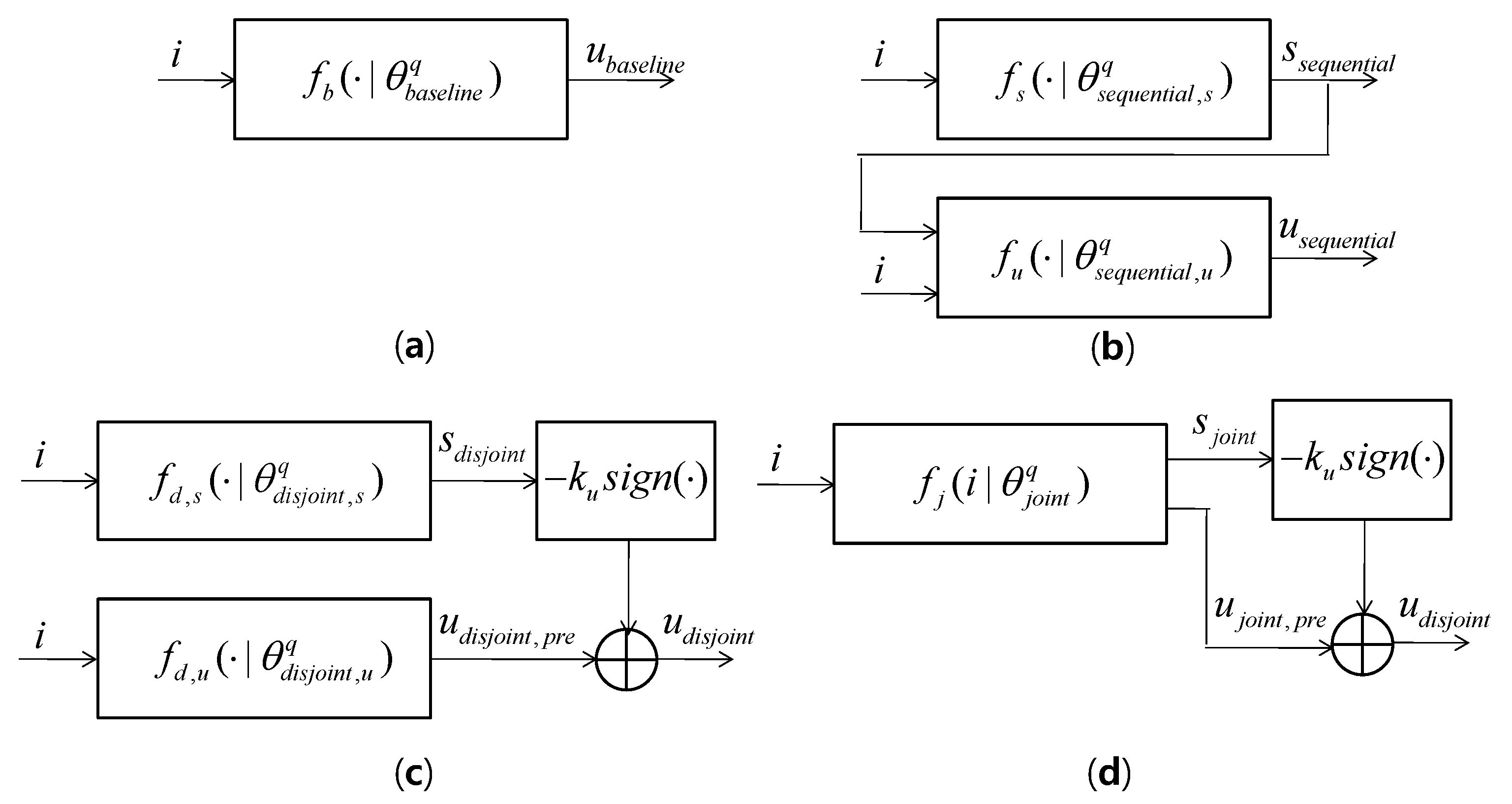
In this section, several DL-based consensus algorithms are proposed. The difference in the proposed consensus algorithms mainly comes from the knowledge adopted in developing a consensus algorithm. All proposed algorithms are designed with the same input to be compared fairly. DL usually requires the input to have the same dimension. However, depending on the number of neighbors, the required information to generate a control signal can be different. Thus, one common rule adopted for designing a neural network is to have separate networks for a different number of neighbors. For example, when the numbers of neighbors in the communication graph are one, two, and three, three different networks will be developed for each algorithm such that each network is dedicated to working on a specific number of neighbors. The structure of the proposed DL-based algorithms at a high level was described in Figure 1:$f_a(\cdot |\theta )$ is a functional abstraction of the neural network of which a set of parameters is represented by $\theta$, where $a$ is a subscript for distinguishing each algorithm with different letters. For example, the single layer network $f_a(\cdot |\theta )$ without activation and bias can be expressed as $f_a(i|\theta )=Wi$ where $i$ is an input to the neural network and $W$ is a weight matrix which can be considered as $\theta$.

3.1. Baseline DL

One of the most naive forms of deep learning for the consensus of MAS is likely to estimate the control signal directly from the input. This network is called the“baseline DL” throughout this paper. An input to the neural network is defined as

$$i_k=\left[\begin{array}{cccc}{e}_k& x_k& {\dot{x}}_k& \begin{array}{cccc}{x}_{{\pi }_k(1)}& {\dot{x}}_{{\pi }_k(1)}& {\ddot{x}}_{{\pi }_k(1)}& \begin{array}{cccc}\cdots & x_{{\pi }_k(Nr(k))}& {\dot{x}}_{{\pi }_k(Nr(k))}& {\ddot{x}}_{{\pi }_k(Nr(k))}\end{array}\end{array}\end{array}\right],$$

(5)

where ${\pi }_k(q)$ is the index of the $q$ th neighbor agent of the agent $k$, and $Nr(k)$ is thenumber of neighbor agents of the agent $k$. The dimension of $i_k$ is $3(Nr(k)+1)$. The selection of input feature is based on the observation of the sliding variables, $s_k^d$ and $s_k^{nd}$, and on the control signals, $u_k^d$ and $u_k^{nd}$, which depend on the elements of $i_k$.Let the baseline DL network used for the agents with $q$ neighbors be denoted as $f_b(i|{\theta }_{baseline}^q)$ where $i$ is the input to the network and ${\theta }_{baseline}^q$ is a set of parameters trained for the baseline DL network. With this definition, the control signal generated by the baseline DL network can be expressed as

$$u_{baseline}=f_b(i|{\theta }_{baseline}^q).$$

(6)

3.2. Sequential DL

The baseline DL network in the previous section does not use any information from designing a control signal. It is observed that the control signals in Equations (3) and (4) depend on a sliding variable. Thus, it may be desirable to predict the sliding variable such that it can be used for predicting the control signal. To this end, two separate networks will be designed such that the first network can predict the sliding variable and the second can predict the control signal with additional information from the first network. This network is called the “sequential DL” throughout this paper. Let the network of the sequential DL used for predicting the sliding variable of the agents with $q$ neighbors be denoted as $f_s(i|{\theta }_{sequential,s}^q)$ where $i$ is the input to the network and ${\theta }_{sequential,s}^q$ is a set of parameters trained for predicting the sliding variable of the sequential DL. With this definition, the sliding variable predicted by the sequential DL can be expressed as

$$s_{sequntial}=f_s(i|{\theta }_{sequential,s}^q).$$

(7)

The predicted sliding variable can be used for predicting the control signal. Let the network of the sequential DL used for predicting the control signal of the agents with $q$ neighbors be denoted as $f_u(i,s_{sequential}|{\theta }_{sequential,u}^q)$ where $i$ is the input to the network and ${\theta }_{sequential,u}^q$ is a set of parameters trained for predicting the control signal of the sequential DL. With this definition, the control signal predicted by the sequential DL can be expressed as

$$u_{sequential}=f_u(i,s_{sequential}|{\theta }_{sequential,u}^q),$$

(8)

3.3. Disjoint DL

Even though the sequential DL uses the predicted sliding variable, it does not use the model structure in the design of the control signal based on sliding mode control. With the intuition that the control performance may get better with more information, a method for explicitly using a control signal structure is considered. This network is called the“disjoint DL” throughout this paper in which two separate networks independently predict the sliding variable and the part of the control signal. Let the network of the disjoint DL used for predicting the sliding variable of the agents with $q$ neighbors be denoted as $f_{d,s}(i|{\theta }_{disjoint,s}^q)$ where $i$ is the input to the network and ${\theta }_{disjoint,s}^q$ is a set of parameters trained for predicting the sliding variable of the disjoint DL. With this definition, the sliding variable predicted by the disjoint DL can be expressed as

$$s_{disjoint}=f_{d,s}(i|{\theta }_{disjoint,s}^q),$$

(9)

$u_k^d$ in (3) can be decomposed into two parts such that $u_k^d$ can be expressed as $u_{k,pre}^d-k_{u}sign(s_k^d)$. $u_k^{nd}$ can be also decomposed in the same way. With this observation, let the network of the disjoint DL used for predicting the first part of the control signal of the agents with $q$ neighbors be denoted as $f_{d,u}(i|{\theta }_{disjoint,u}^q)$ where $i$ is the input to the network and ${\theta }_{disjoint,u}^q$ is a set of parameters trained for predicting the first part of the control signal of the disjoint DL. With this definition, the first part of the control signal predicted by the sequential DL can be expressed as

$$u_{disjoint,pre}=f_{d,u}(i|{\theta }_{disjoint,u}^q),$$

(10)

Finally, the control signal of the disjoint DL can be expressed with the knowledge of the sliding mode control as

$$u_{disjoint}=u_{disjoint,pre}-k_{u}sign(s_{disjoint}),$$

(11)

3.4. Joint DL

The disjoint DL leverages the knowledge of the sliding mode control. It separately predicts the parts of the control with two independent neural networks. However, since the two parts build on similar input features, they may share some common latent features. In some cases, the performance of DL can be improved through multi-task learning which leverages common feature extraction. Thus, predicting both values from a single network may result in better control performance. This network is called the“joint DL” throughout this paper. Let the network of the joint DL used for predicting both parts of the control signal of the agents with $q$ neighbors be denoted as $f_j(i|{\theta }_{joint}^q)$ where $i$ is the input to the network and ${\theta }_{joint}^q$ is a set of parameters trained for predicting both parts of the control signal of thejoint DL. With this definition, both parts of the control signal predicted by the joint DL and the corresponding control signal can be expressed as

$$(u_{joint,pre},s_{joint})=f_j(i|{\theta }_{joint}^q),$$

(12)

$$u_{joint}=u_{joint,pre}-k_{u}sign(s_{joint}),$$

(13)

3.5. Architecture of the Network

Since the input is a low dimensional vector and the DL problem itself is defined as a prediction problem, a conventional fully connected network with multi layers is considered as a basic architecture of the proposed DL. A linear rectifier function was used as an activation function for all layers except the output layer which did not use an activation function. A loss function for an optimization of the network is defined as a mean squared error.

4. Numerical Results and Discussion

To experiment with the proposed DL-based consensus algorithm, the proposed DLs were trained with train data first. Depending on the types of train data, four different versions of trained DL consensus algorithms were compared for consensus performance. The maximum number of neighbors of each agent is limited to two for simplicity. This means that the DL for degree one and the DL for degree two will be trained separately. For each system configuration, control signals and inputs to the neural network were sampled with a period of 0.001 for both training and testing. The simulation time for generating train data for each configuration was 10 s after which the model-based control achieves the consensus for most of the system configurations. Neural networks for each algorithm were trained with Tensorflow 2.0 in Python. The simulation of MAS was also implemented with Python after training the neural networks was completed. Datasets used for the experiments are available at https://github.com/jy-korea/dataset (accessed on 5 April 2022).

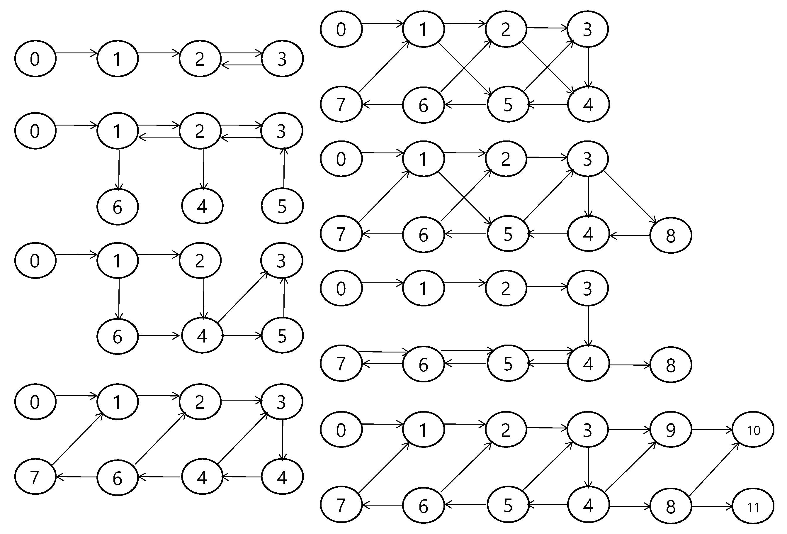
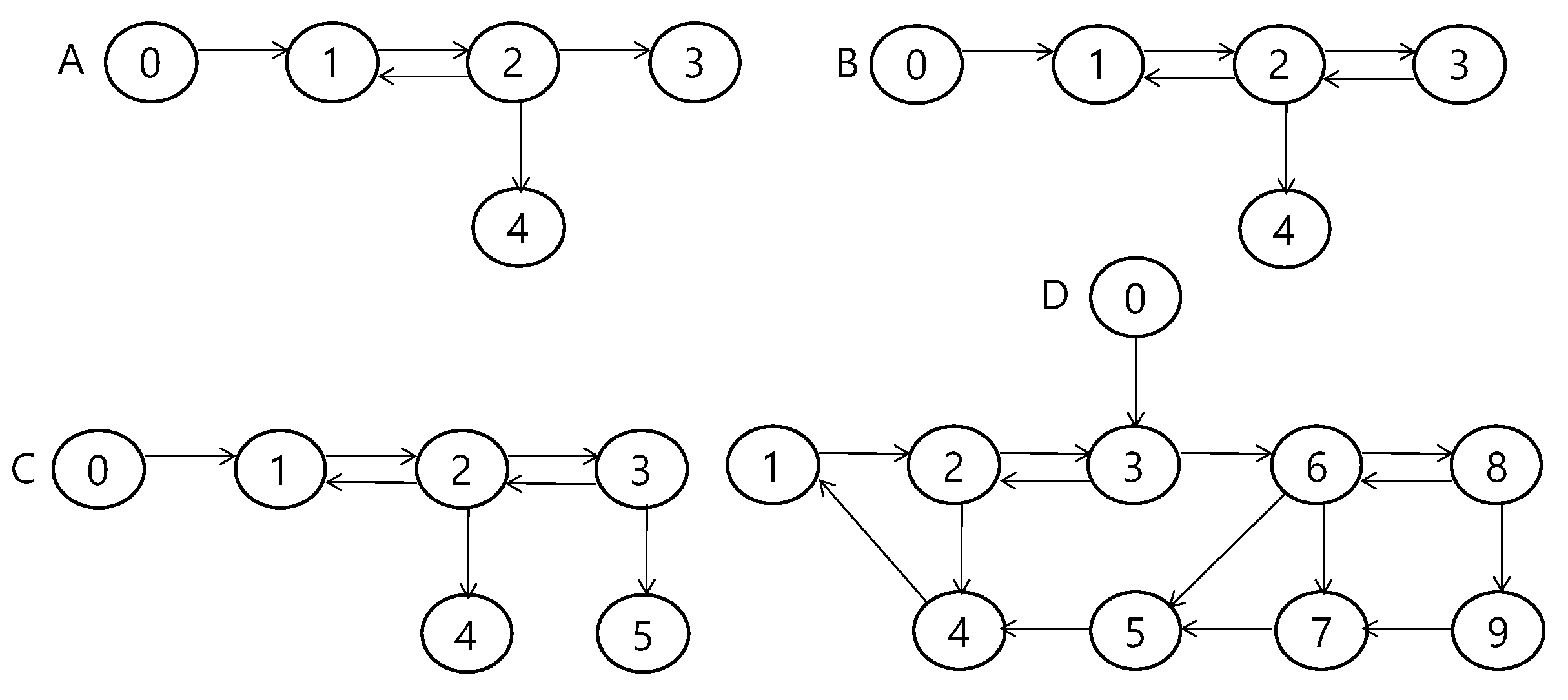
4.1. Train Data Generation

It is very important to have a large number of training data to train a DL network well. To train data, it is also important to have uniformly sampled training data to avoid over-fitting. To this end, train data is generated from varying the leader dynamics, disturbances, and communication graphs. Eight different communication graphs in Figure 2 were used for generating train data. The number of follower agents is 3, 6, 7, 8, or 11. For each communication graph, seven cases with a different acceleration of leader agent and disturbance in

Table 1. Acceleration of leader agent and disturbance used for data generation.

Case	Acceleration of Leader Agent	Disturbance
1	$1/(1+\exp (-0.1gt))$	$\sin (gt)$
2	$\sin (gt)(1+e^{-0.1gt})$	$\cos (gt)[1-e^{-0.1gt}]$
3	$\sin (gt)(1+e^{-t/g}){(1+0.5\cos (gt))}^{-1}$	$\cos (gt)[1-e^{-0.1gt}]$
4	$\sin (gt)(1+e^{-t/g}){(1+0.5\cos (gt))}^{-1}$	$(1+e^{-t/g}){(1+0.5\cos (gt))}^{-1}$
5	$(1+e^{-t/g}){(1+\cos (t)/(g+1))}^{-1}$	$\cos (gt)(1+e^{-t/g}){(1+\cos (gt))}^{-1}$
6	$(1+5e^{-0.1t}){(1+\cos (gt)/(g+1))}^{-1}$	$\sin (gt)(1+e^{-0.1gt})$
7	$(1+5e^{-0.1t}){(1+\cos (gt)/(g+1))}^{-1}$	$\sin (gt)(1+5e^{-0.1gt})$

were simulated. It is observed that the acceleration of leader agent and disturbances are bounded. There can be an infinite number of choices in selecting the acceleration and the disturbance. Even though this choice may not be optimal, it is not particularly bad when it is considered from the simulation results in the subsequent section. Thus, a total of 56 different system configurations were considered. A delay was generated with ${\tau }_{k,l}=a(1+\cos (kt)\sin (lt))$ where $a$ was a parameter to determine the maximum delay. Three different train data were generated. They are called no delay train data, small delay train data, and large delay train data, respectively. The consensus control (3) was used with $a$ being 0 to generate the no delay train data while the consensus control (4) was used with 0.05 and 0.5 to generate the small delay train data and the large delay train data, respectively. Both $k_u$ and $c$ were kept as 10. Finally, each train data has 1,399,860 examples.

4.2. Training the Proposed DL

The hyper-parameters of the fully connected network used for the proposed DL were determined heuristically through trial and error since this research focused on the characterization of supervised learning-based DL for consensus control rather than finding the best DL. Five hidden layers were constructed with each layer having the same number of neurons which is $60(b+1)$ where $b$ is the number of neighbor agents. Thus, network complexity is proportional to the dimension of input. The weighted Adam optimizer with a learning rate of 0.001 and a weight decay of 0.0001 was configured to train the network. The number of epochs was either 50 or 100 at which convergence was confirmed. The MSE performance of DL was not presented since the MSE cannot be a measure for a good DL-based consensus control.

4.3. Simulation Setup

To evaluate the performance of the proposed DL-based consensus control fairly, six different system configurations are considered, They are ssummarized in

Table 2. Acceleration of leader agent, disturbance, and delay used for performance evaluation.

Case	Acceleration of Leader Agent	Disturbance	Graph	Delay
1	$\cos (7t)+\cos (3t)$	$\sin (11t)+\cos (13t)$	A	$0.5{\tau }_{\max }(1+\cos (t+(k+l)\pi /7))$
2	$[\cos (7t)+\cos (3t)](2-e^{-t})$	$\sin (11t)[3-e^{-t}]$	A	$0.5{\tau }_{\max }(1+\cos (111t+(k+l)\pi /7))$
3	$[\cos (7t)+\cos (3t)](2-e^{-t})$	$\sin (11t)[3-e^{-t}]$	B	${\tau }_{\max }{(1+{\mathrm{e}}^{-0.1(k+l)t})}^{-1}$
4	$[\cos (7t)+\cos (3t)](2-e^{-t})$	$\sin (11t)[3-e^{-t}]$	C	${\tau }_{\max }(1-{(1+{\mathrm{e}}^{-0.1(k+l)t})}^{-1})$
5	$[\cos (7t)+\cos (3t)](2-e^{-t})$	$\sin (11t)[3-e^{-t}]$	D	${\tau }_{\max }(1+\cos (t+(k+l)\pi /7)){(2+{\mathrm{e}}^{-0.1(i+j)t})}^{-1}$
6	$\cos (17t)(3-e^{-t}){(2+\cos (13t))}^{-1}$	$\cos (23t)(e^{-0.t}+1)-e^{-t}$	D	${\tau }_{\max }(1-0.5*(1+\cos (t+(k+l)\pi /7)){\mathrm{e}}^{-0.1(k+l)t})$

and Figure 3. To abstract the simulation environment without redundant details, it is assumed that the best way to deal with this comment is to provide the assumption that the individual agents can communicate with each other whilst maintaining their essential autonomy. The system configurations used for generating testing data are different from those for training to have a fair comparison with the model-based consensus algorithm. In Table 2, $k$ and $l$ are the indices of the two agents so that a delay over a communication link can be different, while ${\tau }_{\max }$ is the maximum delay. The initial positions of each agent are randomly selected, while they are the same for all considered algorithms to avoid dependency of performance on initialization. To deal with the delay in the simulation, each agent was initially set to run without control for one second. After applying the proposed consensus algorithms for 10s, which was found to be enough time for convergence, the performance was measured for the final one second.

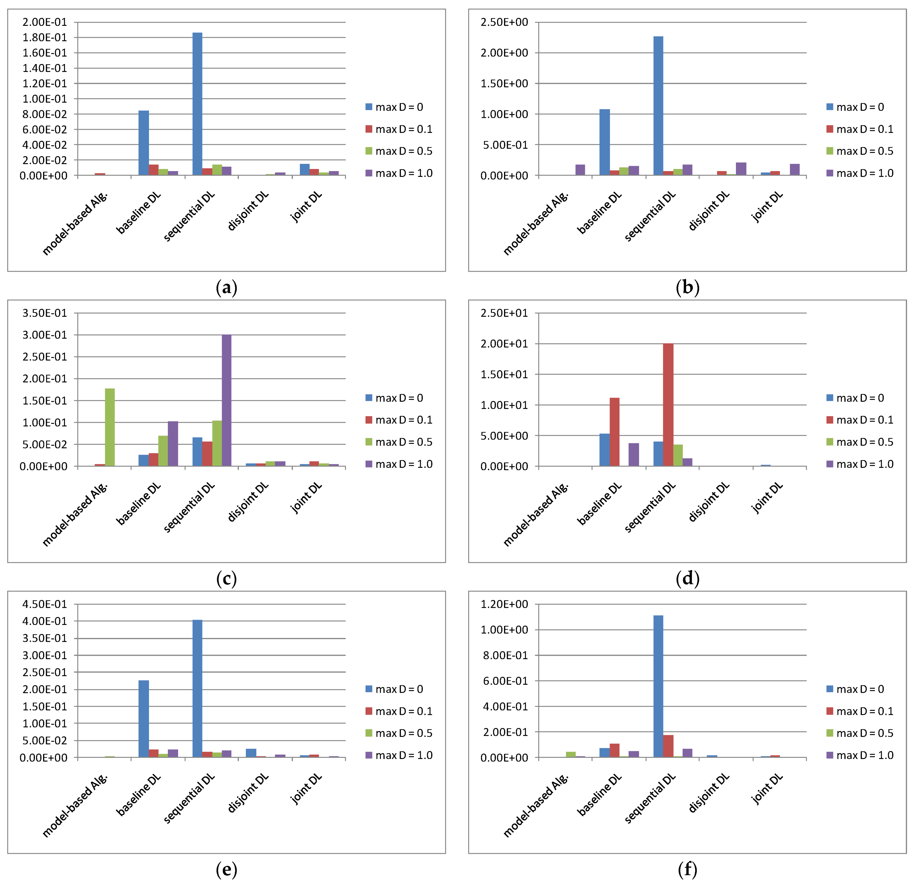
4.4. Simulation Results

The proposed DL consensus algorithms trained with large delay train data were compared with the model-based algorithm presented in Equations (3) and (4). The considered performance metric is the mean square of the disagreement, which is shown in Figure 4 for all simulation cases. It is observed that the model-based algorithm has the mean square of the disagreement close to 0, as it was theoretically proven in [34]. The disjoint DL and the joint DL which explicitlyexploit the sliding mode control structure are found to have better performance than the baseline DL and the sequential DL, while their performances are comparable to that of the model-based DL. It is interesting to note that the mean square of the disagreement of the proposed DLs does not seem to be proportional to the maximum delay as they learn from the model-based control of which performance does not have a dependency on the maximum delay as long as it satisfies some conditions. It is also observed that the disjoint DL and the joint DL have a consistent performance with respect to different delays and the number of agents in a graph. While the baseline DL and the sequential DL provide comparable performance to the model-based for some cases, their performances are marginally worse inmany cases. These results may imply that DL-based consensus control can be further improved with exploiting additional well-crafted side information, whichcan be addressed further in future research.

The proposed DL-based consensus algorithms trained with different train data were compared with the model-based algorithms in Figure 5 and in

Table 3. Average mean square of disagreement over all simulation cases for different train data.

	No Delay Train Data	Small Delay Train Data	Large Delay Train Data
model-based alg.	4.62 × 10−2	7.64 × 10−3	1.82 × 10−2
baseline DL	1.72 × 103	1.28 × 100	9.47 × 10−1
sequential DL	1.49 × 103	1.11 × 100	1.42 × 100
disjoint DL	1.42 × 100	4.55 × 10−1	1.87 × 10−2
joint DL	1.70 × 101	8.68 × 10−2	3.70 × 10−2

. The considered performance metrics are the mean square of the disagreement and the mean square of the displacement from the leader position. The value in Figure 5 is that averaged over sixdifferent cases in Table 2. It was plotted on a log scale to make the results more discernable. As with the large delay train data case, the disjoint DL and the joint DL are found to have a more robust performance than the baseline DL and the sequential DL for the no delay train data and the small delay train data. However, the mean square of disagreement does not seem to be a good measure to represent the degree of the displacement, even though the very large value and the very small value of the mean square of the disagreement are found to be a relatively large value and a relatively small value in the mean square of the displacement. For example, the baseline DL for the maximum delay of 1.0 and the sequential DL for the maximum delay of 0.5 have a similar mean square of the disagreement in Figure 5a. However, they have a very different mean square of the displacement in Figure 5b. Similarly, they have a similar large value of more than 1000 in Figure 5e, while they have a very different value in Figure 5f. These results can be attributed to delay, the nature of the DL-based algorithm, and the multiple edges in a communication graph. Small disagreement in the presence of a delay means the difference between the sum of differences between the delayed neighbor position and the position of an agent is small. Thus, a large delay can incur a large displacement insome cases, particularlyin cases wherethere ismore than one neighbor edge. Since the disagreement is the sum of the differences between the position of an agent and those of its neighbors, the sum of a large positive difference and a large negative difference can result in a small disagreement. Moreover, DL-based algorithms work on a sliding surface learned by train data rather than the actual sliding surface, which is not explicitly defined. Table 3 and

Table 4. Average mean square of displacement from the leader position over all simulation cases for different train data.

	No Delay Train Data	Small Delay Train Data	Large Delay Train Data
model-based alg.	7.03 × 100	5.97 × 100	3.58 × 100
baseline DL	9.66 × 103	2.53 × 101	2.85 × 101
sequential DL	2.10 × 103	2.36 × 101	1.11E × 101
disjoint DL	8.56 × 100	2.05 × 101	3.81 × 100
joint DL	6.69 × 101	9.07 × 100	4.21 × 100

show the mean square of the disagreement and the mean square of the displacement averaged over all simulation cases. It is observed that the disjoint DL and the joint DL with a large delay train data has better performance, while the disjoint DL has a similar performance to that of the model-based for both metrics. It is conjectured that a large delay train data can give an opportunity to find a robust control since the DL-based algorithm may have a chance to explore sample space more uniformly.

Table 5. The execution time for training and for inference for 1000,000 examples.

	Training (s)	Inference (s)
baseline DL	6.11 × 100	1.29 × 101
sequential DL	1.26 × 101	1.27 × 101
disjoint DL	1.26 × 101	2.47 × 101
joint DL	7.77 × 100	1.67 × 101

compares the execution time for training and inference. It was measured on a desktop computer with an Intel i-9 processor, 128GB RAM, and a Nvidia RTX 3090 graphic card. The training time was measured for 1,000,000 examples over 1 epoch. Similarly, the inference time was measured for 1,000,000 examples. Training times for the sequential DL and the disjoint DL are almost twice that of the baseline DL, since these two methods are required to train two networks. The training time of the joint DL is marginally larger than the baseline DL since the network has common lower hidden layers and separate higher hidden layers, which results in a larger number of parameters. It is observed that the inference time for the disjoint DL is twice that of the baseline DL since it consists of two networks. The inference time of the sequential DL is found to be comparable to the baseline DL, which is believed to be parallel processing by the graphic card. In summary, the proposed algorithms are found to have similar computational complexity.

Even though the comparison of the proposed DL-based algorithms with the model- based showed that the proposed algorithms are good enough to be compatible with the model-based, comparison with the RL-based consensus is likely to corroborate the advantage of the proposed algorithms. To this end, the comparison of the disjoint DL with the RL-based consensus was plotted in Figure 6. The maximum delay was set as 0.1 for the simulation. The RL-based algorithm in [41] was implemented after a heuristic search over proper parameterizations, during which the algorithm was found to often diverge and to be very sensitive. The trajectories of each agent can be seen for a system setup corresponding to case 1 in Table 2. Figure 6ashows that the disjoint DL achieves convergence after several seconds while the RL-based algorithm does not for the considered time period. This result is believed to be slow convergence of the RL-based algorithm. To verify the convergence characteristic of the RL-based algorithm, disagreement errors were plotted in Figure 6b,c for the system setup of case 3 in Table 2. For this particular case, the disagreement vector oscillates around 0 after approximately 2s. However, the RL-based algorithm in [41] was found to converge very slowly. It did not seem to converge fully after 30s. This result clearly shows the proposed DL-based algorithm provides a much faster convergence than the RL-based, which is an important issue in the implementation of the consensus algorithm for practical systems.

5. Conclusions

In this paper, several different DL-based consensus control algorithms were proposed. The proposed DL-based consensus algorithms were found to have different performances depending on the degree of knowledge on the control structure. The disjoint DL and the joint DL which explicitly exploit the control structure are found to have better performance in the average mean square error sense. The simulation results also showed that they provided robust performance with respect to different delays, disturbances, and the number of agents in a graph. The performance of the proposed algorithm was shown to depend on the train data. The algorithm trained with large delay train data provided a better performance than with no delay train data and a small delay train data. This implies that, depending on the task, articulated generation of train data is necessitated.

To develop a deep learning-based algorithm with better performance and practical importance, several issues need to be further addressed. Even though the disjoint DL are found to be robust to various system environments, other DL-based algorithms have a better performance in a specific case. Thus, the articulated ensemble model may have provided more robust control, which further improves the performance. Moreover, the proposed DL-based algorithms can be combined with RL so that RL can quicklylearn with the aid of the proposed methods. The DL-based algorithm for a heterogeneous MAS or a nonlinear MAS needs to be studied to make it applicable to many different practical systems.

References

1. Ding, L.; Han, Q.; Ge, X.; Zhang, X. An Overview of Recent Advances in Event-Triggered Consensus of Multiagent Systems. IEEE Trans. Cybern. 2018, 48, 1110–1123. [Google Scholar] [CrossRef] [PubMed] [Green Version]
2. Li, Z.; Duan, Z.; Chen, G.; Huang, L. Consensus of Multiagent Systems and Synchronization of Complex Networks: A Unified Viewpoint. IEEE Trans. Circuits Syst. 2010, 57, 213–224. [Google Scholar] [CrossRef]
3. Nguyen, D.H. A sub-optimal consensus design for multi-agent systems based on hierarchical LQR. Automatica 2015, 55, 88–94. [Google Scholar] [CrossRef]
4. Oh, K.K.; Park, M.C.; Ahn, H.S. A survey of multi-agent formation control. Automatica 2015, 53, 424–440. [Google Scholar] [CrossRef]
5. Li, S.E.; Zheng, Y.; Li, K.; Wang, J. An overview of vehicular platoon control under the four-component framework. In Proceedings of the IEEE Intelligent Vehicles Symposium, Seoul, Korea, 28 June–1 July 2015. [Google Scholar] [CrossRef]
6. Kim, B.; Ahn, H. Distributed Coordination and Control for a Freeway Traffic Network Using Consensus Algorithms. IEEE Syst. J. 2016, 10, 162–168. [Google Scholar] [CrossRef]
7. Trianni, V.; De Simone, D.; Reina, A.; Baronchelli, A. Emergence of Consensus in a Multi-Robot Network: From Abstract Models to Empirical Validation. IEEE Robot. Autom. Lett. 2016, 1, 348–353. [Google Scholar] [CrossRef] [Green Version]
8. Amelina, N.; Fradkov, A.; Jiang, Y.; Vergados, D.J. Approximate Consensus in Stochastic Networks With Application to Load Balancing. IEEE Trans. Inf. Theory 2015, 61, 1739–1752. [Google Scholar] [CrossRef]
9. Zhang, Z.; Gao, Y.; Li, Z. Consensus reaching for social network group decision making by considering leadership and bounded confidence. Knowl. Based Syst. 2020, 204, 106240. [Google Scholar] [CrossRef]
10. Jadbabaie, A.; Lin, J.; Morse, A.S. Coordination of groups of mobile autonomous agents using nearest neighbor rules. IEEE Trans. Autom. Control 2003, 48, 988–1001. [Google Scholar] [CrossRef] [Green Version]
11. Moreau, L. Stability of multi-agent systems with time-dependent communication links. IEEE Trans. Autom. Control 2005, 50, 169–182. [Google Scholar] [CrossRef]
12. Ren, W.; Beard, R.W. Consensus seeking in multi-agent systems under dynamically changing interaction topologies. IEEE Trans. Autom. Control 2005, 50, 655–661. [Google Scholar] [CrossRef]
13. Olfati-Saber, R.; Fax, J.A.; Murray, R.M. Consensus and Cooperation in Networked Multi-Agent Systems. Proc. IEEE 2007, 95, 215–233. [Google Scholar] [CrossRef] [Green Version]
14. Cao, Y.; Ren, W. Optimal Linear-Consensus Algorithms: An LQR Perspective. IEEE Trans. Syst. Man Cybern. Part B Cybern. 2010, 40, 819–830. [Google Scholar] [CrossRef]
15. Yang, D.; Ren, W.; Liu, X.; Chen, W. Decentralized event-triggered consensus for linear multi-agent systems under general directed graphs. Automatica 2016, 69, 242–249. [Google Scholar] [CrossRef] [Green Version]
16. Lomban, D.A.B.; Bernardo, M. Multiplex PI control for consensus in networks of heterogeneous linear agents. Automatica 2016, 67, 310–320. [Google Scholar] [CrossRef] [Green Version]
17. Zhang, D.; Liu, L.; Feng, G. Consensus of Heterogeneous Linear Multiagent Systems Subject to Aperiodic Sampled-Data and DoS Attack. IEEE Trans. Cybern. 2019, 49, 1501–1511. [Google Scholar] [CrossRef]
18. Li, X.M.; Zhou, Q.; Li, P.; Li, H.; Lu, R. Event-Triggered Consensus Control for Multi-Agent Systems Against False Data-Injection Attacks. IEEE Trans. Cybern. 2019, 50, 1856–1866. [Google Scholar] [CrossRef]
19. Wang, Q.; Wang, J.L.; Wu, H.N.; Huang, T. Consensus and H∞ Consensus of Nonlinear Second-Order Multi-Agent Systems. IEEE Trans. Netw. Sci. Eng. 2020, 7, 1251–1264. [Google Scholar] [CrossRef]
20. Zheng, J.; Xu, L.; Xie, L.; You, K. Consensus ability of Discrete-Time Multiagent Systems with Communication Delay and Packet Dropouts. IEEE Trans. Autom. Control 2019, 64, 1185–1192. [Google Scholar] [CrossRef]
21. Olfati-Saber, R. Kalman-Consensus Filter: Optimality, Stability, and Performance. In Proceedings of the 48th IEEE Conference on Decision and Control, Shanghai, China, 16–18 December 2009. [Google Scholar] [CrossRef]
22. Kamal, A.T.; Ding, C.; Song, B.; Farrell, J.A.; Roy-Chowdhury, A.K. A Generalized Kalman Consensus Filter for Wide-Area Video Network. In Proceedings of the 50th IEEE Conference on Decision and Control and European Control Conference (CDC-ECC), Orlando, FL, USA, 12–15 December 2011. [Google Scholar] [CrossRef]
23. Hou, Z.S.; Wang, Z. From model-based control to data-driven control: Survey, classification and perspective. Inf. Sci. 2013, 235, 3–35. [Google Scholar] [CrossRef]
24. Barto, A.G. Reinforcement learning control. Curr. Opin. Neurobiol. 1994, 4, 888–893. [Google Scholar] [CrossRef]
25. Mnih, V.; Kavukcuoglu, K.; Silver, D.; Graves, A.; Antonoglou, I.; Wierstra, D.; Riedmiller, M. Playing atari with deep reinforcement learning. arXiv 2013, arXiv:1312.5602. Available online: https://arxiv.org/abs/1312.5602 (accessed on 5 April 2022).
26. Schulman, J.; Levine, S.; Abbeel, P.; Jordan, M.; Moritz, P. Trust region policy optimization. In Proceedings of the International Conference on Machine Learning, Lille, France, 6–11 July 2015. [Google Scholar]
27. Schulman, J.; Wolski, F.; Dhariwal, P.; Radford, A.; Klimov, O. Proximal policy optimization algorithms. arXiv 2017, arXiv:1707.06347. Available online: https://arxiv.org/abs/1707.06347 (accessed on 9 February 2022).
28. Zhang, H.; Jiang, H.; Luo, Y.; Xiao, G. Data-Driven Optimal Consensus Control for Discrete-Time Multi-Agent Systems with Unknown Dynamics Using Reinforcement Learning Method. IEEE Trans. Ind. Electron. 2017, 64, 4091–4100. [Google Scholar] [CrossRef]
29. Peng, Z.; Hu, J.; Shi, K.; Luo, R.; Huang, R.; Ghosh, B.K.; Huang, J. A novel optimal bipartite consensus control scheme for unknown multi-agent systems via model-free reinforcement learning. Appl. Math. Comput. 2020, 369, 124821. [Google Scholar] [CrossRef]
30. Gao, Y.; Wang, W.; Yu, N. Consensus Multi-Agent Reinforcement Learning for Volt-VAR Control in Power Distribution Networks. IEEE Trans. Smart Grid 2021, 12, 3594–3604. [Google Scholar] [CrossRef]
31. An, N.; Zhao, X.; Wang, Q.; Wang, Q. Model-Free Distributed Optimal Consensus Control of Nonlinear Multi-Agent Systems: A Graphical Game Approach. J. Franklin Inst. 2022, in press. [Google Scholar] [CrossRef]
32. Batra, S.; Huang, Z.; Petrenko, A.; Kumar, T.; Molchanov, A.; Sukhatme, G.S. Decentralized Control of Quadrotor Swarms with End-to-end Deep Reinforcement Learning. arXiv 2017, arXiv:2109.07735. Available online: https://arxiv.org/abs/2109.07735 (accessed on 9 February 2022).
33. Nguyen, T.T.; Nguyen, N.D.; Nahavandi, S. Deep Reinforcement Learning for Multiagent Systems: A Review of Challenges, Solutions, and Applications. IEEE Trans. Cybern. 2020, 50, 3826–3839. [Google Scholar] [CrossRef] [Green Version]
34. Yang, J. A Consensus Control for a Multi-Agent System with Unknown Time-Varying Communication Delays. IEEE Access 2021, 9, 55844–55852. [Google Scholar] [CrossRef]
35. Li, Y.; Li, H.; Wang, S. Finite-Time Consensus of Finite Field Networks with Stochastic Time Delays. IEEE Trans. Circuits Syst. II: Express Briefs 2020, 67, 3128–3132. [Google Scholar] [CrossRef]
36. Wang, X.; Wang, H.; Li, C.; Huang, T.; Kurths, J. Consensus Seeking in Multiagent Systems with Markovian Switching Topology Under Aperiodic Sampled Data. IEEE Trans. Syst. Man Cybern. Syst. 2020, 50, 5189–5200. [Google Scholar] [CrossRef]
37. Ahmed, S.F.; Raza, Y.; Mahdi, H.F.; Muhamad, W.M.W.; Joyo, M.K.; Shah, A.; Koondhar, M.Y. Review on Sliding Mode Controller and Its Modified Types for Rehabilitation Robots. In Proceedings of the 6th International Conference on Engineering Technologies and Applied Sciences (ICETAS), Kuala Lumpur, Malaysia, 20–21 December 2019. [Google Scholar] [CrossRef]
38. Yu, S.; Long, X. Finite-time consensus for second-order multi-agent systems with disturbances by integral sliding mode. Automatica 2015, 54, 158–165. [Google Scholar] [CrossRef]
39. Qin, J.; Zhang, G.; Zheng, W.X.; Kang, Y. Adaptive Sliding Mode Consensus Tracking for Second-Order Nonlinear Multiagent Systems with Actuator Faults. IEEE Trans. Cybern. 2019, 49, 1605–1615. [Google Scholar] [CrossRef]
40. Zhang, J.; Lyu, M.; Shen, T.; Liu, L.; Bo, Y. Sliding Mode Control for a Class of Nonlinear Multi-agent System with Time Delay and Uncertainties. IEEE Trans. Ind. Electron. 2018, 65, 865–875. [Google Scholar] [CrossRef]
41. Li, J.; Ji, L.; Li, H. Optimal consensus control for unknown second-order multi-agent systems: Using model-free reinforcement learning method. Appl. Math. Comput. 2021, 410, 126451. [Google Scholar] [CrossRef]
Figure 1. The structure of the proposed DL-based consensus control (a) baseline DL; (b) sequential DL; (c) disjoint DL; (d) joint DL.
Electronics 11 01176 g001
Figure 2. Communication graphs used for train data generation.
Electronics 11 01176 g002
Figure 3. Communication graphs used for performance evaluation.
Electronics 11 01176 g003
Figure 4. The mean square of disagreement of the proposed DL consensus algorithm trained with large delay train data (max D is the maximum delay τ max ) (a) case 1; (b)case 2; (c)case 3; (d)case 4; (e)case 5; (f) case 6.
Electronics 11 01176 g004
Figure 5. The mean square of disagreement and the mean square of the displacement from the leader position of the proposed DL consensus algorithms trained with different train data (max D is the maximum delay τ max ) (a) the mean square of disagreement—no delay train data; (b) the mean square of the displacement from the leader position—no delay train data; (c) the mean square of disagreement—small delay train data; (d) the mean square of the displacement from the leader position—small delay train data; (e) the mean square of disagreement—large delay train data; (f) the mean square of the displacement from the leader position—large delay train data.
Electronics 11 01176 g005
Figure 6. Comparison of the disjoint DL with the RL-based algorithm by Li, 2021 (a) state trajectory for case 1; (b) disagreement error of the disjoint DL for case 3; (c) disagreement error of the RL-based algorithm in [41] for case 3.
Electronics 11 01176 g006