Optimal Scheduling of Time-Sensitive Networks for Automotive Ethernet Based on Genetic Algorithm

Abstract

In this paper, we proposed a scheduling method to optimize a time-critical traffic using genetic algorithm in automotive ethernet networks. The proposed traffic scheduling method aims to generate a transmission schedule to minimize end-to-end delay, variation of reception time at the destination (jitter), and bandwidth utilization. These indicators should be simultaneously considered when generating a schedule since they are closely related to the performance of the networks. However, it is not easy to schedule the traffic considering these indicators together since they have different sizes and units. To solve this problem, the fitness function to evaluate performance of a chromosome has normalized indicators as parameters. A chromosome in the genetic algorithm consists of genes containing information (size, transmission period, and network delay) of messages to be scheduled. Finally, the applicability of the proposed schedule optimization method was examined by simulating an extended automotive Ethernet network for an autonomous vehicle.

1. Introduction

In recent years, to satisfy level three or higher autonomous driving levels defined by the Society of Automotive Engineers, vehicles should have a high level of stability and reliability [1]. These vehicles navigate using information obtained from many advanced driver-assistance-system sensors and the vehicle’s external infrastructure. However, the rapidly increasing information for autonomous driving requires a high network bandwidth that cannot be supported by existing vehicle network technologies such as the Control Area Network and FlexRay [2,3]. Furthermore, since the loss and latency of time-critical data in a network can adversely affect the control of autonomous driving vehicles, a vehicle network that can reliably transmit time-critical data in real-time is required for these vehicles [4,5,6,7,8].

For the fulfilment of the high requirements for autonomous driving networks, considerable attention has been paid to the ethernet protocol. The widely known ‘ethernet standard’ has been evolving to support high bandwidths and various traffic types, and its applicability extends from office environments to the aerospace and automotive industries and smart factories [9]. Generally, ethernet provides a best effort delivery service in which messages within a given bandwidth are transmitted regardless of the frame importance. However, this service may involve frame loss or high delay as the network traffic increases, and this may cause serious problems for autonomous vehicles, which should make decisions based on the most up-to-date and complete information for safe and reliable autonomous driving. Thus, an improved ethernet technology is required to guarantee the reliability and real-time transmission of time-critical traffic for autonomous vehicles.

Deterministic ethernet, which was proposed to improve the limitations of conventional ethernet, offers accurate time synchronization between devices in a network, extremely low frame loss, and bounded delay time [10]. Time-sensitive networking (TSN) is one of the deterministic ethernet technologies. Some of the sub-standards of the IEEE 802.1 ethernet standard established by the IEEE TSN task group support time synchronization, stream reservation, seamless redundancy, frame preemption, and scheduled traffic. In particular, scheduled traffic based on time synchronization can minimize the delay in a transmission queue for time-critical traffic, and guarantee bounded latency and real-time response even in a congested network.

IEEE 802.1Qbv for TSN is a standard related to scheduled traffic, and it specifies the transmission mechanism of scheduled traffic (ST) in an egress port [11]. In IEEE 802.1Qbv, the network traffic can be divided into eight queues at an egress port according to priority, and transmission is determined according to the queue state. Here, the queue state is determined to be open or closed by the time scheduler in the gate controller list (GCL). IEEE 802.1Qbu, which is another standard associated with scheduling, prioritizes ST transmission through frame preemption, even if the network is occupied by another traffic [12]. Using these standards, autonomous driving networks can transmit high-priority control and sensor messages according to a predefined schedule and minimize delays [13].

In a general network environment, ST is delivered to the destination via several links in its path. Therefore, in all links used for ST transmission, the transmission timing should be scheduled to guarantee real-time transmission through the minimization of the end-to-end delay of ST [14]. This task is similar to job shop schedule problem with NP-hard complexity [15]. If we need to schedule n ST messages on a link, we will have n! possible schedules. In addition, if these ST messages have to travel over m links, we will have almost (n!)^m choices that can amount to a significantly large number. Various scheduling approaches have been proposed to solve the schedule optimization problem of deterministic ethernet. Generally, to solve the traffic scheduling problem in the networks, many researchers proposed mathematical techniques such as integer programming (ILP) or satisfiability modulo theories. Santos et al. proposed a scheduling technique involving a satisfiability modulo theories (SMT) solver to generation automated schedule for TSN [16]. Craciunas et al. formalized the scheduling problem using logical constraints and proposed an optimization method based on SMT and maximum intensity projection [17]. Pang et al. proposed a schedule generation mechanism to achieve update transmission consistency using an enhanced ILP method [18]. Shen et al. have researched on synchronization and state estimation issues of complex dynamic networks (CDNs) for stabilization [19,20]. However, these approaches are limited since the scheduling problem is classified as an NP-complete problem. Although new and powerful methods based on mathematical techniques have been proposed, they are still difficult to formulate [21,22]. Gavriluţ applied the greedy randomized adaptive search procedure to schedule all TSN and AVB traffic in industrial applications [23]. Furthermore, Durr defined critical data scheduling as a no-wait job shop scheduling problem and proposed a schedule compression algorithm that reduced the wasted bandwidth utilization due to the guard band [24].

This paper proposes a method for optimizing a traffic scheduling problem in an environment that simulates a time-synchronized autonomous driving network. The method employs a genetic algorithm. In particular, ST was expressed as a gene to apply the genetic algorithm to the traffic scheduling problem. Scheduling was performed according to the order of ST frames in the gene, which was represented by a Gantt chart, and the final schedule was created by applying schedule compression to reduce the number of occurrences of guard bands in the complete schedule. The performance of the schedule was evaluated by using a fitness function involving three performance indicators: end-to-end (E2E) delay of ST, jitter, and bandwidth utilization for the guard band (BUGB). The fitness function was calculated using a weighted sum of the normalized performance indicators. Finally, an autonomous driving network was simulated to evaluate the optimization algorithm’s performance and applicability. The contributions of this paper are summarized as follows:

(1)

We assumed that the scheduling problem in TSN is to find an appropriate schedule order of ST, and it has been shown through simulation that it can be solved with a genetic algorithm using order-based representation.

(2)

To optimize the schedule, fitness function is defined as weighted sum of normalized indicators; end-to-end delay, jitter, and BUGB. This means that the ST can be scheduled by reflecting three indicators at once, and scheduling will be able to consider network requirements by adjusting the weights.

(3)

The proposed approach is simulated in the topology of autonomous vehicle networks and verified for its applicability.

This paper consists of six sections. In Section 2, the network model used for scheduling is explained, and in Section 3 the genetic algorithm (GA) used for scheduling optimization is elucidated. Section 4 describes the GA-based schedule optimization algorithm, and in Section 5 the performance evaluation environment and results are discussed. Finally, Section 6 presents our conclusions.

2. Network Model for Scheduling

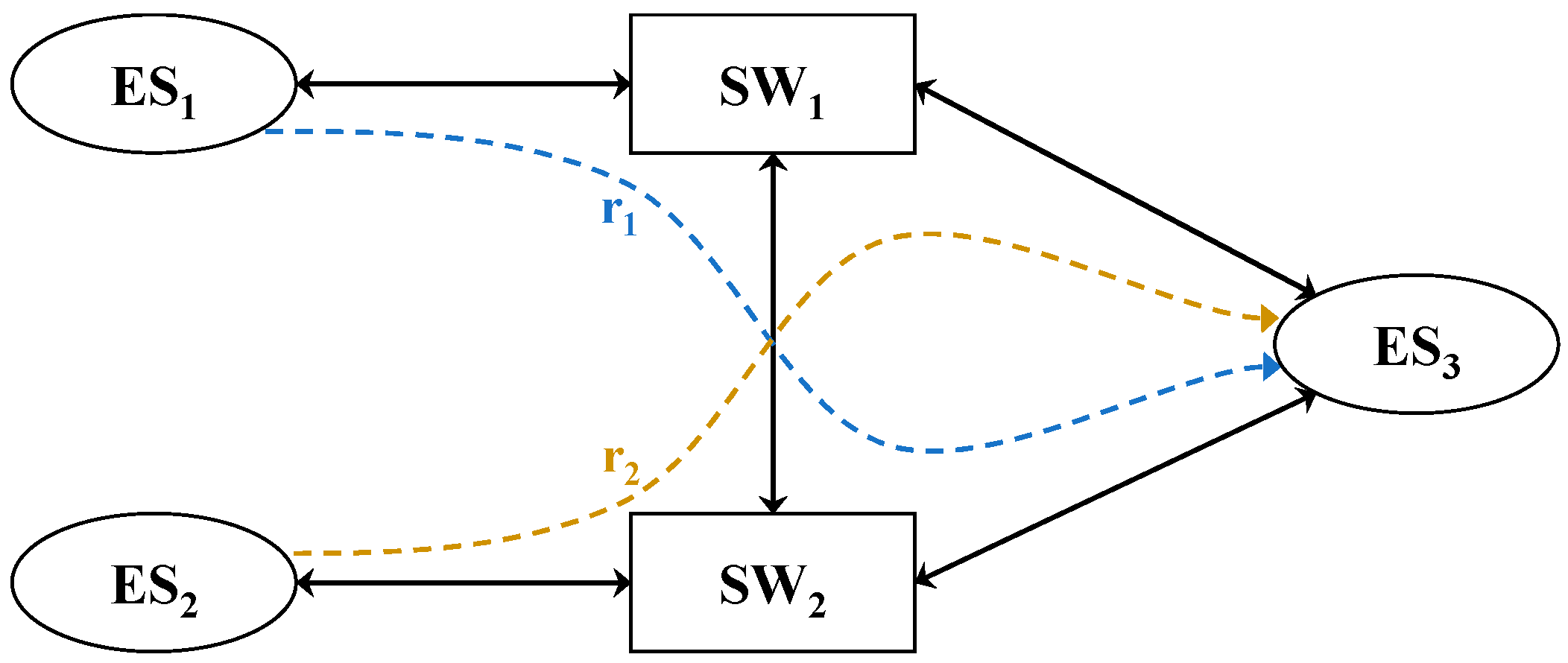
2.1. Architecture Model

An architecture model that represents a physical connection in a network with abstraction and that includes end systems (ESs), switches (SWs), and links can be modeled using a directed graph $\mathcal{G}\left(E, V\right)$ [25]. Here, $V$ (vertices) represents ESs and SWs, which are devices in the network, and is defined as $V=ES\cup SW$. $E$ (edge) refers to a physical data link, and when $v_a,v_b\in V$, a link connected from $v_a$ to $v_b$ can be expressed as $\left[v_a,v_b\right]\in E$. Each edge has three attributes: transmission rate, propagation delay, and queue number. Here, the transmission rate means the number of bits transmitted per second in the link, which is defined as $\left[v_a,v_b\right].s$. The propagation delay refers to the time that it takes for the electrical signal to reach the destination from the source through physical media, and it is expressed as $\left[v_a,v_b\right].d$. Finally, the queue number refers to the number of queues in an egress port. In the TSN standard, up to eight queues are permitted in an egress port. Here, the $n$th queue in an egress port is expressed as $\left[v_a,v_b\right].n$. Figure 1 shows a network topology consisting of three ESs and two SWs. The traffic transmission route is denoted by $r_k$, which refers to an ordered sequence of edges from the source to the destination when traffic is transmitted. For $r_1$ in Figure 1, the source is ES1 and the destination is ES3, and the route can be expressed in terms of a list of edges as $r_1=\left(\left[E{S}_1, S{W}_1\right],[S{W}_1, S{W}_2\left], [S{W}_1, E{S}_3\right]\right)$.

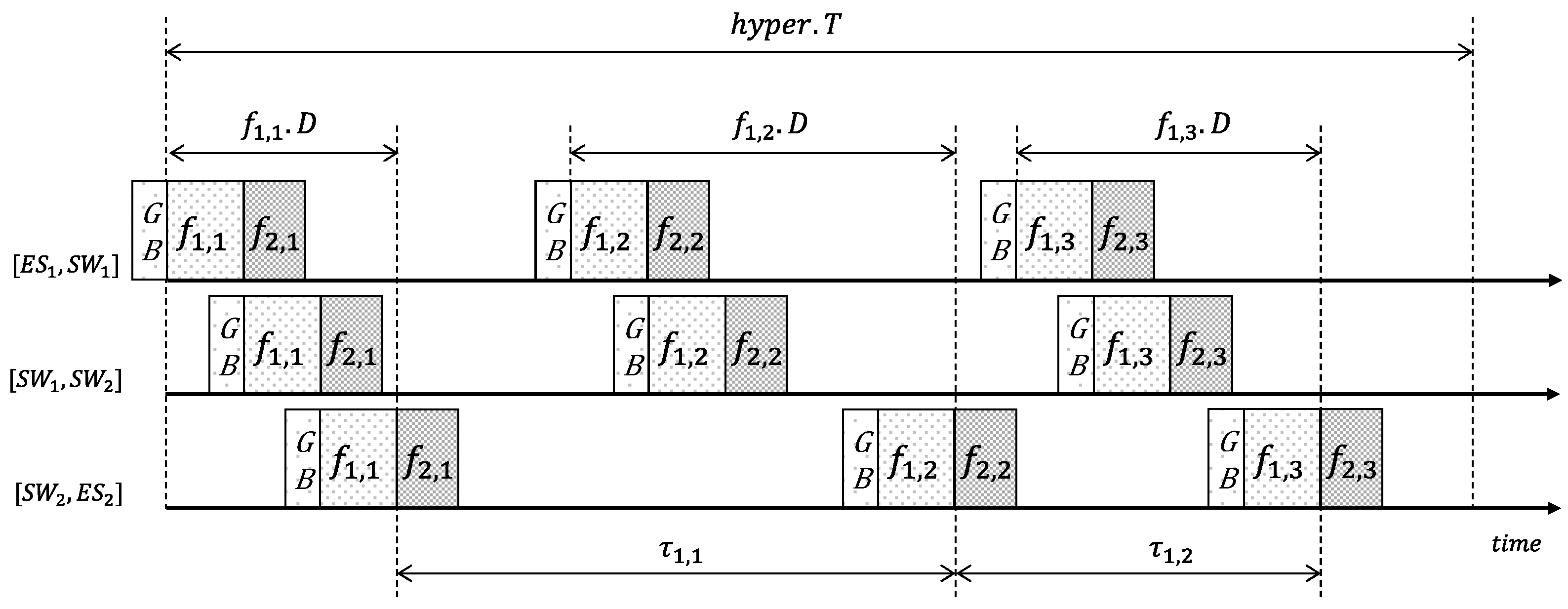
2.2. Application Model

An application model represents information about messages required for TSN scheduling and time information required to operate the GCL, and it is expressed as $\mathcal{T}\left(\mathit{S},\mathit{C}\right)$. The parameter $\mathit{S}$ is a set of flows $s_i$, with $s_i\in \mathit{S}$. Here, flow $s_i$ is an abstract expression of messages transmitted periodically in a specific route. In this paper, $s_i$ is defined as the $i$th ST. The flow transmission period and flow transmission route are expressed as $s_i.T$ and $s_i.r_k$, respectively. The parameter $\mathit{C}$ refers the open or closed state of the GCL, and the GCL state is determined by the schedule. Frame transmission is allowed only while the corresponding gate is open.

Frame $f$, with $f\in \mathit{F}$, is a unit of data exchanged in the Ethernet network, and $\mathit{F}$ denotes a set of frames. The $m$th frame of flow $s_i$ transmitted through link $\left[v_a,v_b\right]$ is denoted by $f_{i,m}^{\left[v_a,v_b\right]}$, where the frame size is expressed as $f_{i,m}^{\left[v_a,v_b\right]}.B$. Equation (1) presents the expression for the network delay $f_{i,m}^{\left[v_a,v_b\right]}.D$ when a frame is transmitted through a link $\left[v_a,v_b\right]$. The network delay is defined as the sum of the processing delay, queuing delay, transmission delay, and propagation delay. Here, the processing delay, expressed as $f_{i,m}^{\left[v_a,v_b\right]}.p$, refers to the time taken to determine the destination by checking the header when the frame is received at $v_a$ and checking the error. The transmission delay is expressed as $f_{i,m}^{\left[v_a,v_b\right]}.t$, which is the value of frame size $f_{i,m}^{\left[v_a,v_b\right]}.B$ divided by the transmission rate $\left[v_a,v_b\right].s$. The last term in Equation (1) denotes propagation delay that equals to the physical length of $\left[v_a,v_b\right]$ divided by the speed of electromagnetic or optical signal.

$$f_{i,m}^{\left[v_a,v_b\right]}.D=f_{i,m}^{\left[v_a,v_b\right]}.p+f_{i,m}^{\left[v_a,v_b\right]}.q+f_{i,m}^{\left[v_a,v_b\right]}.t+\left[v_a,v_b\right].d$$

(1)

The bandwidth utilization rate $f_{i,m}^{\left[v_a,v_b\right]}.U$ per second by a frame, which is the frame size divided by the transmission rate, is given by

$$f_{i,m}^{\left[v_a,v_b\right]}.U=\frac{f_{i,m}^{\left[v_a,v_b\right]}.B}{\left[v_a,v_b\right].s}$$

(2)

Equation (3) presents an expression for the frame reception completion time $f_{i,m}^{\left[v_a,v_b\right].n}.R$ at the $n$th queue of the egress port at $v_a$, and $f_{i,m}^{\left[v_a,v_b\right].n}.R$ is the sum of the network delay $f_{i,m}^{\left[v_a,v_b\right]}.D$ and the frame reception completion time $f_{i,m}^{\left[v_{\overline{a}},v_a\right].n}.R$ at the queue $\left[v_{\overline{a}},v_a\right].n$ in the immediately previous link. The frame reception completion time $f_{i,m}^{\left[v_a,v_b\right].n}.R$ is used as a variable to determine whether frames collide during the schedule generation process.

$$f_{i,m}^{\left[v_a,v_b\right].n}.R=f_{i,m}^{\left[v_{\overline{a}},v_a\right].n}.R+f_{i,m}^{[v_a,v_b]}.D$$

(3)

3. Genetic Algorithm for TSN Scheduling

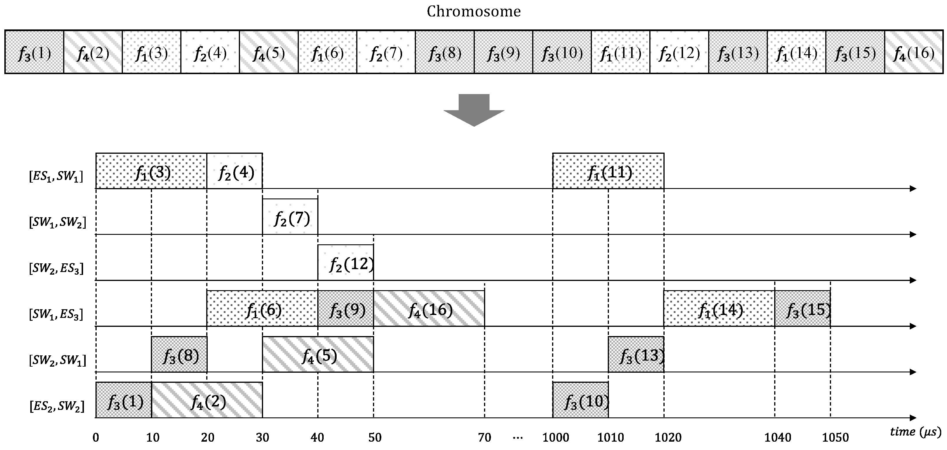
3.1. Chromosome Representation

GA represents a problem solution as a form of chromosomes consisting of genes and finds the optimal chromosome to solve the problem through the evolution mechanism [26]. In the present study, chromosome refers to frames of ST arranged following the order of consideration in the schedule generation process. That is, the first (last) gene in the chromosome represents the frame of ST that is considered first (last) in the schedule generation process. Since the performance of the schedule is determined by the order of genes in the chromosome, the scheduling result can be improved by optimizing the order of genes [27].

In the GA used for schedule optimization, the chromosome length $(CL$) represents the total number of frames transmitted during the hyper period ($hyper.T$) for all routers in the network. Here, $hyper.T$ refers to the shortest period of which the transmission pattern of all flows is repeated, and it is calculated as the least common multiple (LCM) of the periods of all flows, as expressed in Equation (4). Finally, $CL$ can be calculated as in Equation (5) where the value of $hyper.T$ divided by $s_i.T$ means how many times a flow $s_i$ should be sent during $hyper.T$ and $num\left(s_i.r\right)$ is the number of links a flow should cross to reach its destination.

$$hyper.T=LCM\left(\forall s_i.T\right)$$

(4)

$$CL={\displaystyle \sum }_{\forall s_i}\left\{\frac{hyper.T}{s_i.T}\times num\left(s_i.r\right)\right\}$$

(5)

Table 1. Attributes of frames on the network shown in Figure 1.

Frame	Period (ms)	Network Delay (us)	Route
$f_1$	1000	20	[ES1, SW1] [SW1, ES3]
$f_2$	2000	10	[ES1, SW1] [SW1, SW2] [SW2, ES3]
$f_3$	1000	10	[ES2, SW2] [SW2, SW1] [SW1, ES3]
$f_4$	2000	20	[ES2, SW2] [SW2, SW1] [SW1, ES3]

presents the period, the transmission delay, and a route example of the frames transmitted in the network in Figure 1. Using this information, $hyper.T$ and the length of the chromosome required for chromosome generation can be calculated. Figure 2 shows an example of a chromosome created using the information in Table 1. The created chromosome consists of 16 genes, and the schedule is performed in sequence according to the denoted number.

3.2. Fitness Function

GA should define an appropriate fitness function for the problem to be solved since the chromosomes in current generation should be evaluated for transferring superior chromosomes to the next generation. This study selected three indicators directly relevant to the performance of the TSN network over which scheduling was performed. The selected performance indicators were a frame’s end-to-end (E2E) delay, bandwidth utilization by guard bands (BUGB), and reception jitter at the destination. Since the performance indicators had different units and different semantics with each other, they were normalized for use as parameters in the fitness function.

3.2.1. End-To-End Delay

The E2E delay refers to the sum of all delays in the transfer of a frame from the source to the destination node. Since the E2E delay of each frame varies with the number of hops in the link through which the frame passes, an additional calculation process is required. Equation (6) presents the E2E delay performance indicator. The term $f_{i,m}^{s_i.r}.D_{real}$ is the measured E2E delay when a frame is transmitted according to the schedule, and $f_{i,m}^{s_i.r}.D_{ideal}$ is defined as the E2E delay under the assumption that there is no queuing delay, i.e., there is no other frames when the frame is transmitted. Here, the E2E delay performance indicator was calculated as the sum of the ratios of the difference between the real $f_{i,m}^{s_i.r}.D_{real}$ and the ideal $f_{i,m}^{s_i.r}.D_{ideal}$ to $f_{i,m}^{s_i.r}.D_{ideal}$. The variable n refers to the number of flows, and $k_i$ refers to the number of the frames transmitted during the hyper period in the $i$th flow.

$$E2Edelay={\displaystyle \sum }_{i=1}^n\{{\displaystyle \sum }_{m=1}^{k_i}(\frac{f_{i,m}^{s_i.r}.D_{real}-f_{i,m}^{s_i.r}.D_{ideal}}{f_{i,m}^{s_i.r}.D_{ideal}})\}$$

(6)

3.2.2. Jitter

Jitter refers to the variation in E2E delay (it is also called latency variation). In this study, the jitter represented the deviation in the interval between successive frame reception instants at the destination during the hyper period. It was defined as zero for frames that were transmitted only once during the hyper period. Equation (7) presents the jitter performance indicator, which is the mean of the jitters of all frames. Here, ${\tau }_{i,m}$ is the difference between the reception times of the $m$th and $\left(m+1\right)$th frames at the destination in the flow $s_i$ during the hyper period, $\overline{\tau }$ is the mean of ${\tau }_{i,m}$ measured during the hyper period, $k_i$ is the number of frames in the flow $s_i$, and $n$ refers to the number of flows.

$$Jitter=\frac{1}{n}{\displaystyle \sum }_{i=1}^n\sqrt{{\displaystyle \sum }_{m=1}^{k_i-1}\left(\frac{{\left({\tau }_{i,m}-\overline{\tau }\right)}^2}{k_i}\right)}$$

(7)

3.2.3. Bandwidth Utilization by Guard Bands

To prevent the interference of non-ST with ST transmission, IEEE 802.1Qbv blocks the former by setting the guard band of the maximum frame size (MFS, 1542 bytes) before transmitting ST at the defined time on the transmission schedule [12]. This guarantees the bounded latency of critical frames. It should be noted that guard band is not needed when two or more STs are transmitted successively. IEEE 802.1Qbu can reduce the guard band size to 124 bytes through frame preemption [12]. In any case, an increase in the number of guard bands could cause waste of network bandwidth. Thus, a schedule to minimize the guard band count is required. The right-hand side of Equation (8) is the ratio of the sum of the transmission times of all guard bands in a link to the hyper period. In the equation, $l\in E$ denotes the links in the network, $GB.cn{t}_l$ is the guard band count used in link $l$, $GB.size$ is the guard band size in bits, and $rate.l$ is the transmission speed of link $l$.

$$BUGB=\frac{1}{hyper.T}{\displaystyle \sum }_{\forall l\in E}\frac{GB.cn{t}_l\times GB.size}{rate.l}$$

(8)

Figure 3 shows an example of a schedule represented by a Gantt chart; frame $f_1$ is transmitted thrice. The E2E delay of $f_1$ is $f_{1,i}.D$ (i = 1, 2, 3), and the reception interval of successive frames is represented by ${\tau }_{1,j}$ (j = 1, 2). The guard band count can be checked since the guard band occurs before the frame transmission for each link.

4. Scheduling of Time-Sensitive Networks for Automotive Ethernet

4.1. Schedule Generation Method

Information required for schedule generation is acquired from the architecture model and the application model. The chromosome is made up of frames of ST which are represented as genes and the frames on each chromosome are initially arranged randomly. Next, the schedule is generated by placing a frame on the links from its source to destination on the Gannt chart, in the order of frames of the chromosome. For schedule generation, the transmission route of the frames, size, and period should be considered. A frame should be placed as earliest as possible, and if it is scheduled on a link over the route, the schedule on the next link should start from the transmission completion time on the preceding link. In addition, a frame should be placed immediately after the end of transmission of another frame being transmitted on the same link. The complete schedule, with all of the ST in the chromosome represented on the Gantt chart, can be generated by repeating the above method. Figure 4 shows the Gantt chart created during schedule generation for the chromosome in Figure 2. The sequence number is mentioned after the frame number to indicate the scheduling order. Since $f_3$ is the first frame in Figure 2, it is placed on $\left[E{S}_2,S{W}_2\right]$ according to the route in Table 1, and $f_4$, which is represented as the second gene, is arranged in the same link. Frame $f_1$, which is represented as the third gene, is placed on $\left[E{S}_1,S{W}_1\right]$. This process is iterated to obtain the result in Figure 4.

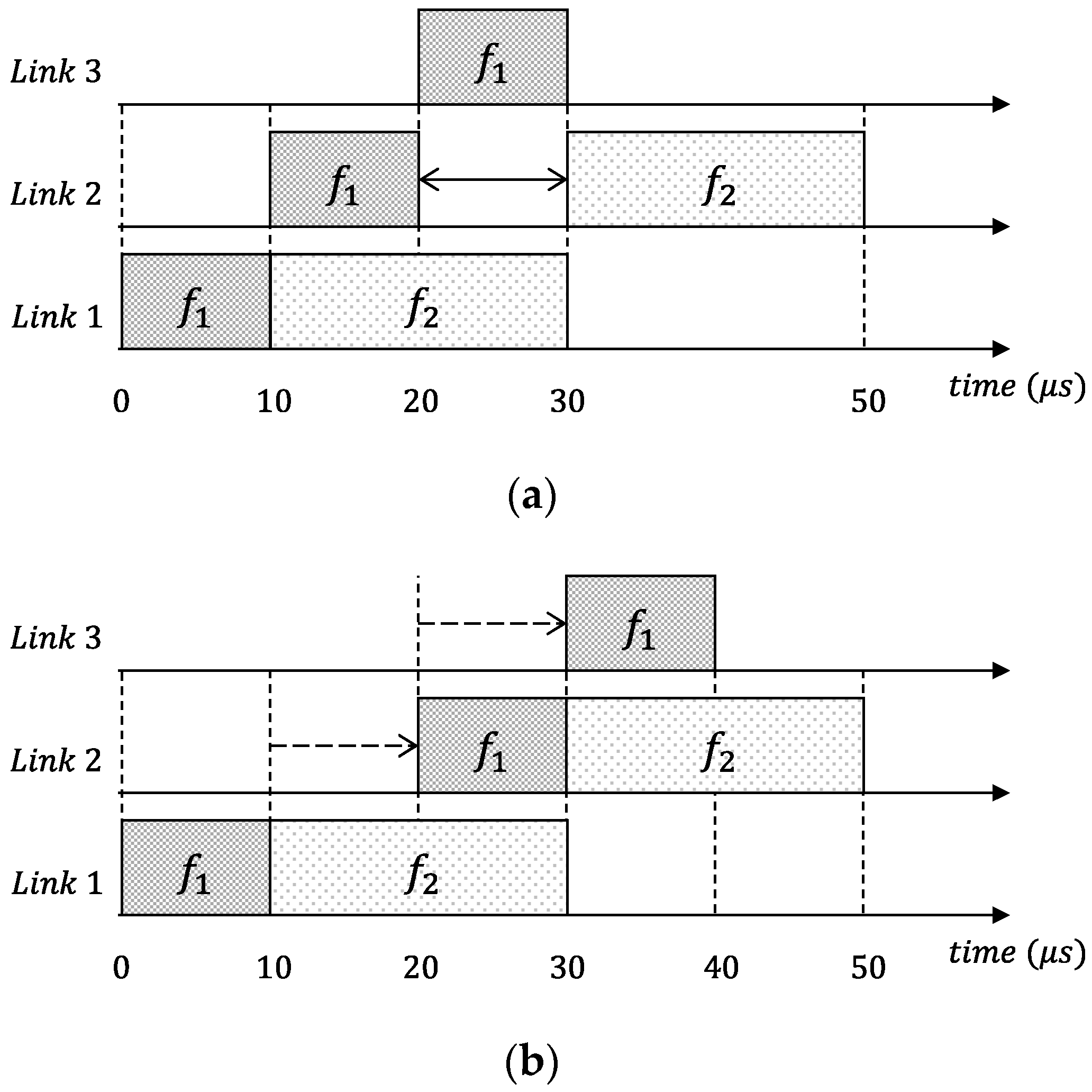
4.2. Schedule Compression Method

The schedule generated for the chromosome may have slacks between frames. For example, in Figure 4, a slack of 10 µs is present between frames $f_3$ and $f_4$ in the link $\left[S{W}_2,S{W}_1\right]$. Since the guard band is required just before a consecutive block of ST frames, more guard bands are generated if there are slacks between frames of ST. Unnecessary guard bands waste the network bandwidth. Thus, it is necessary to minimize slacks between frames of ST by compressing the schedule.

Schedule compression starts from searching for slacks after generating a schedule for all frames. It is then determined whether a detected slack can be compressed and, if it can be compressed, the frame location of the preceding message can be shifted toward to the following message by an amount equal to the slack. For example, in Figure 4, $f_3\left(8\right)$ on link $\left[S{W}_2,S{W}_1\right]$ can be delayed until the transmission start time on link $\left[S{W}_1,E{S}_3\right]$ without increasing E2E delay. Therefore, $f_3\left(8\right)$ on link $\left[S{W}_2,S{W}_1\right]$ can be pushed towards immediately before $f_4\left(5\right)$, thereby reducing the guard band count. However, there may be some cases where the slack cannot be compressed in the Gantt chart. Figure 5 shows a case where the schedule cannot be compressed. In the figure, if the slack on link 2 is compressed by adjusting the transmission start time of $f_3$, it affects the transmission start time of $f_3$ on link 3, thereby increasing the E2E delay. Therefore, compression cannot be carried out. In summary, schedule compression should be performed only when it does not affect the final arrival times of ST framed.

4.3. Parameter Normalization for Fitness Function

On the basis of the schedule obtained through schedule generation and compression, the schedule performance for the current chromosome can be measured by performing a fitness evaluation. For the fitness, the E2E delay, jitter, and BUGB are used as performance indicators. However, these three performance indicators have different units and different semantics with each other. Therefore, it is necessary to normalize them before using them in the fitness function. For this, a large number of chromosomes are randomly generated, and their performance indicators are used as a basis of normalization. It turns out that these performance indicators follow a normal distribution. Thus, the performance indicators obtained from a chromosome could be converted into a z-score of the standard normal distribution using the mean and standard deviation of the randomly generated samples that followed a normal distribution. The performance indicators obtained in the normalization process were used as the parameters in the fitness function; they were expressed as $Fitnes{s}_D$, $Fitnes{s}_J$, and $Fitnes{s}_{GB}$. Finally, the final $Fitnes{s}_{total}$ used to evaluate the performance of the chromosome was defined as a weighted sum of the parameters as follows.

4.4. GA-Based Optimal Scheduling Algorithm

Figure 6 shows a flowchart of the optimal schedule optimization algorithm using GA. The schedule optimization algorithm is divided into three parts: the creation of a generation with a large population, schedule generation from chromosomes and fitness calculation, and GA operation to obtain a chromosome with superior traits from the current generation. Initially, the current generation is defined after iteratively creating a chromosome with a random arrangement of genes until the population reaches n. Then, a schedule is generated for each population of the current generation and their fitness values are calculated. A new generation is created by performing the selection, crossover, and mutation operations to acquire a superior chromosome in the GA operation part. Finally, the algorithm is performed as many as m times to find the optimal chromosome, and it returns the best-performance chromosome in the last generation.

The GA operation selects the 25% of the best-fit chromosomes through elitism selection and transfers them to the next generation. It then performs tournament selection for the rest of the chromosomes by randomly pairing them. Here, chromosome selection was performed as follows: two chromosomes are randomly selected along with a random number in the range [0, 1], and if this number was smaller than the selection pressure, a chromosome with higher fitness was selected. Otherwise, a chromosome with lower fitness was selected. The chromosomes selected for the next generation exchange their genes with others through the crossover operation, thereby hopefully acquiring better chromosomes. Here, the precedence preserving order-based crossover (POX) in which information exchange is based on the order of the genes was employed for the gene operator used for the crossover [28]. Figure 7 shows an example of the POX operation. This operation preserves the locations of certain number of STs in the chromosome (in this example, two STs). Two chromosomes are randomly selected from the current generation and designated as parents 1 and 2, respectively. For these parents, two pairs of STs are randomly chosen and stored in J1 and J2. Then, the locations of STs stored in J1 in parent 1 are copied to the corresponding locations in offspring 1, and the remaining positions are filled with STs of the parent 2, excluding those stored in J1, sequentially from the left to the right direction, as shown in Figure 7a. Figure 7b shows the creation process of offspring 2. The POX has the advantage that the order of genes in a chromosome is preserved when the genes are transferred to the offspring, resulting in the characteristics of the parents being reproduced, to some extent, in the offspring. Furthermore, reverse mutation, in which the gene arrangement order is reversed, was used for the mutation operator to minimize the local minima problem.

5. Experiments

For the evaluation of the proposed algorithm, a network for an autonomous driving system for large vehicles such as buses was considered. The network consisted of 17 end stations and four switches, as shown in Figure 8. The 17 end stations consisted of cameras, radars, LIDAR, and controllers. All links in the network were set with 100 Mbps Ethernet full-duplex.

Table 2. Characteristics of flows on the network.

Traffics	Source	Destination	Period (ms)	Size (Byte)	Network Delay (us)	Route
1	LRR	DCU	50	125	10	[LRR, SW1], [SW1, DCU]
2	CAM1	DCU	20	750	60	[CAM1, SW4], [SW4, SW3], [SW3, DCU]
3	CAM2	DCU	20	750	60	[CAM2, SW4], [SW4, SW3], [SW3, DCU]
4	CAM3	DCU	20	750	60	[CAM3, SW4], [SW4, SW3], [SW3, DCU]
5	CAM4	DCU	20	750	60	[CAM4, SW4], [SW4, SW3], [SW3, DCU]
6	MRR1	DCU	50	125	10	[MRR1, SW2], [SW2, DCU]
7	MRR2	DCU	50	125	10	[MRR2, SW2], [SW2, DCU]
8	MRR3	DCU	50	125	10	[MRR3, SW2], [SW2, DCU]
9	MRR4	DCU	50	125	10	[MRR4, SW2], [SW2, DCU]
10	MRR5	DCU	50	125	10	[MRR5, SW2], [SW2, DCU]
11	LIDAR	IVN	20	363	29	[LIDAR, SW1], [SW1, IVN]
12	LIDAR	DCU	20	363	29	[LIDAR, SW1], [SW1, DCU]
13	LIDAR	ADR	20	363	29	[LIDAR, SW1], [SW1, SW3], [SW3, ADR]
14	MAP	DCU	100	625	50	[MAP, SW3], [SW3, DCU]
15	IVN	DCU	10	250	20	[IVN, SW1], [SW1, DCU]
16	IVN	LRR	10	250	20	[IVN, SW1], [SW1, LRR]
17	IVN	MRR1	10	250	20	[IVN, SW1], [SW1, SW2], [SW2, MRR1]
18	IVN	MRR2	10	250	20	[IVN, SW1], [SW1, SW2], [SW2, MRR2]
19	IVN	MRR3	10	250	20	[IVN, SW1], [SW1, SW2], [SW2, MRR3]
20	IVN	MRR4	10	250	20	[IVN, SW1], [SW1, SW2], [SW2, MRR4]
21	IVN	MRR5	10	250	20	[IVN, SW1], [SW1, SW2], [SW2, MRR5]
22	DCU	IVN	10	250	20	[DCU, SW1], [SW1, IVN]
23	DCU	IVN	20	250	20	[DCU, SW1], [SW1, IVN]
24	V2X	MAP	20	250	20	[V2X, SW4], [SW4, MAP]
25	V2X	DCU	100	250	20	[V2X, SW4], [SW4, SW3], [SW3, DCU]
26	ADR	DCU	100	500	40	[ADR, SW3], [SW3, DCU]
27	HVI	DCU	100	125	10	[HVI, SW3], [SW3, DCU]

LRR, long-range radar; DCU, domain control unit; CAMn, camera #n; MRR, mid-range radar; IVN, gateway for in-vehicle network; ADR, automatic data recorder; MAP, map and positioning; V2X, vehicle to infrastructure; HVI, human-vehicle interface.

presents information related to 27 flows transmitted over the network.

The population, which refers to the number of chromosomes generated when the GA was run, was set to 96 chromosomes per generation, and the evolution process was performed for over 50 generations. Furthermore, the selection pressure and mutation rate were set to 0.9 and 0.05, respectively. Figure 9 shows the average and minimum fitness for different generations created when the proposed TSN schedule algorithm was applied to the network in Figure 8. Here, the fitness was calculated as a weighted sum (α = 0.5, β = 0.3, and γ = 0.2) of the performance indicators represented by z-scores. The lower the value, the better the performance. It was important to consider the most recent output of the sensors for autonomous driving; 0.5 was selected for α, which was the weight value of the E2E delay, and 0.3 was selected for β since sensor information had to be provided on a regular basis. Since the network traffic was not very large compared with the capacity of the network, γ, which was the weight of the loss due to the guard band, was set to a relatively low value, 0.2.

The chromosome that showed the best performance over the 50 generations appeared from the 46th generation, and the variation of the average fitness revealed that the diversity of the chromosome was properly maintained. The total calculation time of the GA for schedule optimization was around 12,300 s, and the calculation was performed in a personal computer with CPU-i5 and 8 GB random access memory.

Figure 10 shows the normal distributions of each performance indicator. To represent each indicator as z-score, the normal distribution used 1000 chromosome as samples. Here, in order to generate different schedules, chromosome samples are generated by randomly arranging genes. In the figure, solid vertical lines represent the best performance indicator results that corresponds to the minimum fitness obtained for the 46th generation in Figure 9. The performance results after running the GA showed that the performance indicators E2E delay, jitter, and BUGB were 6.5559 × 10⁻³, 1.5061 µs, and 9.3272 × 10⁻³ (around 0.93%), respectively. Here, the E2E delay had no unit since it was calculated as a ratio between real and ideal values through the scheduling [29].

Table 3. Heuristic and GA-based scheduling results.

Method	$\mathit{F}\mathit{i}\mathit{t}\mathit{n}\mathit{e}\mathit{s}{\mathit{s}}_{\mathit{D}}$	$\mathit{F}\mathit{i}\mathit{t}\mathit{n}\mathit{e}\mathit{s}{\mathit{s}}_{\mathit{J}}$	$\mathit{F}\mathit{i}\mathit{t}\mathit{n}\mathit{e}\mathit{s}{\mathit{s}}_{\mathit{G}\mathit{B}}$	$\mathit{F}\mathit{i}\mathit{t}\mathit{n}\mathit{e}\mathit{s}{\mathit{s}}_{\mathit{T}\mathit{o}\mathit{t}\mathit{a}\mathit{l}}$
GA	−2.2772	−2.8884	−1.2000	−2.2451
Heuristic	−0.3967	−2.0155	−1.4000	−1.0830

shows $Fitnes{s}_D$, $Fitnes{s}_J$, and $Fitnes{s}_{GB}$, i.e., the z-scores of the performance indicators, E2E delay, jitter, and BUGB, respectively, and their weighted sum $Fitnes{s}_{total}$. The result obtained through the GA-based schedule is compared with that of a heuristic-based schedule [30]. In the heuristic method used here, the scheduling starts with the flow with the highest priority by placing frames on all links over the route of the flow during the hyper period, and this process was iteratively performed in the order of the highest priority for the others. As presented in Table 3, $Fitnes{s}_{Total}$ of the GA-based algorithm was −2.2451, which showed better performance than the heuristic method (−1.0830). This indicated that the GA-based method was more effective than the method that created a schedule according to the priority of the flows. More specifically, the E2E delay was the most improved performance indicator when the GA was applied. The z-score of E2E delay (−2.2772) obtained by the proposed algorithm approximately corresponds to top 1.13% while that of the heuristic method means top 34.5% based on the normal distribution. However, $Fitnes{s}_{GB}$ showed worse performance than the heuristic method. Among many reasons, this was due to the fact that in the calculation of $Fitnes{s}_{Total}$, the lowest weight was given to $Fitnes{s}_{GB}$.

6. Conclusions

This paper proposes a GA-based schedule optimization method for real-time transmission of time-critical data in a TSN network. In the GA, genes in a chromosome were matched with frames that had to be scheduled during the hyper period. The schedule was created according to the order of the genes arranged in a chromosome, and guard band was minimized through the compression process to reduce slacks after creating the schedule for all frames. To evaluate the schedule performance, three performance indicators (E2E delay, jitter, and BUGB) were selected. All of the performance indicators were found to follow a normal distribution for randomly generated 1000 chromosomes. On the basis of this result, normalization was conducted for the three performance indicators, which had different units and different semantics with each other. The GA was applied using $Fitnes{s}_{Total}$, which was calculated as a weighted sum of the normalized performance indicators, namely, $Fitnes{s}_D$, $Fitnes{s}_J$, and $Fitnes{s}_{GB}$.

For the evaluation of the performance of the proposed schedule optimization method, a network for an autonomous commercial vehicle was considered for numerical experiments. The network consists of 17 end nodes and four switches, and accommodates 27 different types of flows. Finally, schedule results obtained with a heuristic method and with the proposed schedule optimization method were compared, and the following conclusions were drawn from the experimental results.

First, in this paper, we proposed a GA method for optimal scheduling for the TSN. More specifically, an order of flows to be scheduled was represented with an order of genes in a chromosome rather than the schedule itself being represented with a chromosome structure. For the evaluation of the schedule performance, the E2E delay, jitter, and BUGB were considered. For the normalization of the performance indicators, which had different units and absolute values, the normal performance distribution of the randomly generated schedules was used.

Second, the performance of the schedule obtained using the GA was better than the schedule that was randomly created and the schedule created with a heuristic method. The total sum of the fitness for the proposed method was compared with that for the heuristic method, and it showed a significant improvement from −1.0830 to −2.2451. In particular, the E2E delay, whose weight was the largest, showed a significant improvement. The above results hinted that the proposed method could be applied to real problems since the study results were obtained for a relatively practical case in which 27 types of flows were transmitted by connecting 17 end stations to four switches.

Nonetheless, the proposed method has limitations that considered only ST that is real-time traffic but not considered other traffic classes such as RC (rate constrained) and BE (best effort) in a TSN network. Since RC and BE can also affect schedule results, in future studies, they should be included. Furthermore, the calculation time would significantly increase with the network size and the final result from the proposed method cannot be guaranteed to not be a local minimum. In addition, for the practical implementation of the proposed method, hardware components (ECUs, sensors, and switches etc.) which support the function of TSN schedule are required. In the future, we plan to evaluate the impact of improved network performance on the vehicle stability through the proposed scheduling method.

References

1. SAE Standard J3016; SAE Taxonomy and Definitions for Terms Related to Driving Automation Systems for On-Road Motor Vehicles. SAE: Warrendale, PA, USA, 2018.
2. Hank, P.; Müller, S.; Vermesan, O.; Van Den Keybus, J. Automotive Ethernet: In-vehicle networking and smart mobility. In Proceedings of the Design, Automation & Test in Europe Conference & Exhibition, Grenoble, France, 18–22 March 2013; pp. 1735–1739. [Google Scholar]
3. Hank, P.; Suermann, T.; Müller, S. Automotive Ethernet, a holistic approach for a next-generation in-vehicle networking standard. In Advanced Microsystems for Automotive Applications; Springer: Berlin/Heidelberg, Germany, 2012; pp. 79–89. [Google Scholar]
4. Uhlemann, E. Introducing connected vehicles. IEEE Veh. Technol. Mag. 2015, 10, 23–31. [Google Scholar]
5. Kim, M.H.; Lee, S.; Ha, K.N.; Lee, K.C. Implementation of a fuzzy-inference-based low-speed, close-range collision warning system for the urban area. Proc. Inst. Mech. Eng. Part D 2013, 227, 234–245. [Google Scholar] [CrossRef]
6. Doecke, S.; Grant, A.; Anderson, W.G. The real-world safety potential of connected vehicle technology. Traffic Inj. Prev. 2015, 16, 531–535. [Google Scholar] [CrossRef] [PubMed]
7. Zolock, J.; Senatore, C.; Yee, R.; Larson, R.; Curry, B. The Use of Stationary Object Radar Sensor Data from Advanced Driver Assistance Systems (ADAS) in Accident Reconstruction; SAE Technical Paper 2016, 2016-01-1465; SAE: Warrendale, PA, USA, 2016. [Google Scholar]
8. Lee, K.C.; Lee, S.; Lee, M.H. Worst case communication delay of real-time industrial switched Ethernet with multiple levels. IEEE Trans. Ind. Electron. 2006, 53, 1669–1676. [Google Scholar] [CrossRef]
9. Sommer, J.; Gunreben, S.; Feller, F.; Kohn, M.; Mifaoui, A.; Sass, D.; Scharf, J. Ethernet—A survey on its fields of application. IEEE Commun. Surv. Tutor. 2010, 12, 263–284. [Google Scholar] [CrossRef] [Green Version]
10. Bruckner, D.; Stănică, M.; Blair, R.; Schriegel, S.; Kehrer, S.; Seewald, M. An Introduction to OPC UA TSN for industrial communication systems. Proc. IEEE 2019, 107, 1121–1131. [Google Scholar] [CrossRef]
11. IEEE 802.1Qbv; Bridges and Bridged Networks—Amendment 25: Enhancements for Scheduled Traffic. IEEE-SA: New York, NY, USA, 2015.
12. IEEE 802.1Qbu; Bridges and Bridged Networks—Amendment 26: Enhancements for Frame Preemption. IEEE-SA: New York, NY, USA, 2016.
13. Wan, T.; Ashwood-Smith, P. A performance study of CPRI over Ethernet with IEEE 802.1Qbu and 802.1Qbv enhancements. In Proceedings of the IEEE Global Communication Conference, San Diego, CA, USA, 6–10 December 2015; pp. 1–6. [Google Scholar]
14. Atallah, A.A.; Hamad, G.B.; Mohamed, O.A. Routing and Scheduling of Time-Triggered Traffic in Time-Sensitive Networks. IEEE Trans. Ind. Inform. 2020, 16, 4525–4534. [Google Scholar] [CrossRef]
15. Tindell, K.W.; Burns, A.; Wellings, A.J. Allocating hard real-time tasks: An NP-hard problem made easy. Real-Time Syst. 1992, 4, 145–165. [Google Scholar] [CrossRef]
16. Dos Santos, A.C.T.; Schneider, B.; Nigam, V. TSNSCHED: Automated Schedule Generation for Time Sensitive Networking. In Proceedings of the 2019 Formal Methods in Computer Aided Design (FMCAD), San Jose, CA, USA, 22–25 October 2019; pp. 69–77. [Google Scholar]
17. Craciunas, S.S.; Oliver, R.S.; Chmelík, M.; Steiner, W. Scheduling real-time communication in IEEE 802.1Qbv time sensitive networks. In Proceedings of the RTNS ‘16: Proceedings of the 24th International Conference on Real-Time Networks and Systems, Brest, France, 19–21 October 2016; pp. 183–192. [Google Scholar]
18. Pang, Z.; Huang, X.; Li, Z.; Zhang, S.; Xu, Y.; Wan, H. Flow Scheduling for Conflict-Free Network Updates in Time-Sensitive Software-Defined Networks. IEEE Trans. Ind. Inform. 2021, 17, 1668–1678. [Google Scholar] [CrossRef]
19. Liu, Y.; Xiz, J.; Meng, B.; Song, X.; Shen, H. Extended dissipative synchronization for semi-Markov jump complex dynamic networks via memory sampled-data control scheme. J. Frankl. Inst. 2020, 357, 10900–10920. [Google Scholar] [CrossRef]
20. Wang, Y.; Hu, X.; Shi, K.; Song, X.; Shen, H. Network-based passive estimation for switched complex dynamical networks under persistent dwell-time with limited signals. J. Frankl. Inst. 2020, 357, 10921–10936. [Google Scholar] [CrossRef]
21. Falk, J.; Dürr, F.; Rothermel, K. Exploring Practical Limitations of Joint Routing and Scheduling for TSN with ILP. In Proceedings of the 2018 IEEE 24th International Conference on Embedded and Real-Time Computing Systems and Applications (RTCSA), Hakodate, Japan, 28–31 August 2018; pp. 136–146. [Google Scholar]
22. Jones, A.; Rabelo, L.C.; Sharawi, A.T. Survey of Job Shop Scheduling Techniques; NISTIR; National Institute of Standards and Technology: Gaithersburg, MD, USA, 1999. [Google Scholar]
23. Gavriluţ, V.; Pop, P. Scheduling in time sensitive networks (TSN) for mixed-criticality industrial applications. In Proceedings of the 2018 14th IEEE International Workshop on Factory Communication Systems (WFCS), Imperia, Italy, 13–15 June 2018; pp. 1–4. [Google Scholar]
24. Dürr, F.; Nayak, N.G. No-wait Packet Scheduling for IEEE Time-sensitive Networks (TSN). In Proceedings of the RTNS ’16: Proceedings of the 24th International Conference on Real-Time Networks and Systems, New York, NY, USA, 19–21 October 2016; pp. 203–212. [Google Scholar]
25. Raagaard, M.M.; Pop, P. Optimization Algorithm for the Scheduling of IEEE 802.1 Time-Sensitive Networking (TSN); Technical Report; Technical University of Denmark: Lyngby, Denmark, 2017; Available online: http://www2.compute.dtu.dk/~paupo/publications/Raagaard2017aa-Optimization%20algorithms%20for%20th-.pdf (accessed on 10 February 2022).
26. Whitley, D. A genetic algorithm tutorial. Stat. Comput. 1994, 4, 65–85. [Google Scholar] [CrossRef]
27. Moghadam, A.M.; Wong, K.Y.; Piroozfard, H. An efficient genetic algorithm for flexible job-shop scheduling problem. In Proceedings of the 2014 IEEE International Conference on Industrial Engineering and Engineering Management, Selangor, Malaysia, 9–12 December 2014; pp. 1409–1413. [Google Scholar]
28. Lee, K.M.; Yamakawa, T.; Lee, K.M. A genetic algorithm for general machine scheduling problems. In Proceedings of the 1998 Second International Conference, Knowledge-Based Intelligent Electronic Systems, Proceedings KES’98 (Cat. No.98EX111), Adelaide, Australia, 21–23 April 1998; Volume 2, pp. 60–66. [Google Scholar]
29. Kim, H.J.; Lee, K.C.; Lee, S. A Genetic Algorithm based Scheduling Method for Automotive Ethernet. In Proceedings of the IECON 2021—47th Annual Conference of the IEEE Industrial Electronics Society, Toronto, ON, Canada, 13–16 October 2021; pp. 1–5. [Google Scholar]
30. Kim, H.J.; Choi, M.H.; Kim, M.H.; Lee, S. Development of an Ethernet-Based Heuristic Time-Sensitive Networking Scheduling Algorithm for Real-Time In-Vehicle Data Transmission. Electronics 2021, 10, 157. [Google Scholar] [CrossRef]
Figure 1. Example of a simple time-sensitive networking (TSN) topology.
Electronics 11 00926 g001
Figure 2. Example of chromosome generated using the information in Table 1.
Electronics 11 00926 g002
Figure 3. Example of performance indicators in a schedule represented in a Gantt chart.
Electronics 11 00926 g003
Figure 4. Case of schedule generated from chromosome in Gantt chart.
Electronics 11 00926 g004
Figure 5. Cases where schedule compression is not possible: (a) before compression and (b) after compression.
Electronics 11 00926 g005
Figure 6. Flowchart of the GA-based TSN optimal schedule method.
Electronics 11 00926 g006
Figure 7. Examples of the POX operation: (a) offspring 1 and (b) offspring 2.
Electronics 11 00926 g007
Figure 8. Network topology used for the performance evaluation of the genetic-algorithm-based TSN optimal schedule algorithm. LRR, long-range radar; DCU, domain control unit; CAMn, camera #n; MRR, mid-range radar; IVN, gateway for in-vehicle network; ADR, automatic data recorder; MAP, map and positioning; V2X, vehicle to infrastructure; HVI, human-vehicle interface.
Electronics 11 00926 g008
Figure 9. Average and minimum fitness variation during the operation of the algorithm.
Electronics 11 00926 g009
Figure 10. Best performance metrics compared with random schedules.
Electronics 11 00926 g010