A Hybrid Routing Protocol Based on Naïve Bayes and Improved Particle Swarm Optimization Algorithms

Abstract

Clustering of sensor nodes is a prominent method applied to wireless sensor networks (WSNs). In a cluster-based WSN scenario, the sensor nodes are assembled to generate clusters. The sensor nodes also have limited battery power. Therefore, energy efficiency in WSNs is crucial. The load on the sensor node and its distance from the base station (BS) are the significant factors of energy consumption. Therefore, load balancing according to the transmission distance is necessary for WSNs. In this paper, we propose a hybrid routing algorithm based on Naïve Bayes and improved particle swarm optimization algorithms (HRA-NP). The cluster heads (CHs) are selected according to the CH conditional probability, which is estimated by the Naïve Bayes classifier. After the selection of the CHs, the multi-hop routing algorithm is applied to the CHs. The best routing path from each CH to the BS is obtained from an improved particle swarm optimization (PSO) algorithm. Simulations were conducted on evaluation factors such as energy consumption, active sensor nodes per round, the sustainability of the network, and the standard deviation of a load on the sensor node. It was observed that HRA-NP outperforms comparable algorithms, namely DUCF, ECRRS, and FC-RBAT, based on the evaluation factors.

1. Introduction

A wireless sensor network (WSN) is a multi-hop self-organizing network composed of a large number of microsensors with a dynamic topology. Data gathering and transmission are the main goals of WSNs [1]. By integrating different types of sensors, such as temperature, humidity, and pressure sensors, for data acquisition and monitoring, WSNs can be used in medical treatments, industry, environmental protection, agriculture, etc. [2]. Because WSN nodes are powered by a battery, energy-efficient utilization is the key component of WSN design and optimization [3,4]. On the other hand, due to the complex occlusion and other characteristics of the network’s application environment, the data transmission process between WSN nodes is vulnerable to interference and the influence of the surrounding environment, and the link characteristic is a probabilistic connectivity state of time connection and time disconnection. In recent years, many researchers have carried out energy consumption optimization research on routing path selection in wireless sensor networks. Cluster head multi-hop hybrid routing based on a cluster structure is a current research hotspot [5]. In this hybrid routing structure, the nodes are first clustered locally, then the data collected by the sensing nodes are collected by the cluster head, and finally the data are returned to the base station (BS) through multiple hops between cluster heads [6]. The advantage of the hybrid routing structure is that it can simplify the network’s structure and effectively avoid energy consumption hotspots and energy consumption funnels. The cluster head is the key node in the hybrid routing structure [7]. Cluster head selection and multi-hop path selection between cluster heads are key to determining the overall energy consumption performance of the network [8].

The routing protocol proposed in this paper considers cluster head selection and multiple hops between cluster heads in unreliable link networks. A machine learning method is adopted in order to select the cluster head and the multi-hop path according to the node residual energy, link quality, and hops for the purpose of saving energy. In unreliable link networks, a relay node and path selection problem can be transformed into a characteristic probability problem of nonlinear classification. In this paper, a classification method based on a Naïve Bayes algorithm is used to establish a relay selection method for energy consumption optimization. The classification method based on the Naïve Bayes algorithm is a very efficient machine learning method that is widely used in various application scenarios.

2. Related Works

2.1. Clustering Routing Algorithms

A cluster routing protocol divides the monitored area into a set of nodes called clusters. In each cluster, one or more nodes are selected to be cluster heads in a certain way, and the nodes in the cluster perform data communication with the BS through the cluster head. After the network adopts a cluster structure, the network is divided into multiple relatively independent clusters, which reduces the impact of the change in the network topology on the system and improves the stability and maintainability of the network. The cluster head can fuse the data in the cluster before forwarding them, which reduces the amount of data transmitted and the network’s energy consumption [9,10].

Clustering routing algorithms have the advantages of a simple structure, efficient topology management, and no requirement for complex routing information. The classical clustering routing protocol LEACH [11] uses ordinary nodes as cluster heads in a probabilistic way, which balances the additional energy consumption of cluster heads to a certain extent and prolongs the network’s lifetime. The advantage of the LEACH algorithm lies in the simplicity of the cluster head selection algorithm because the random selection of a cluster head cannot ensure the dispersion of the cluster head’s position and sufficient residual energy, which can easily cause an imbalance in the network node energy consumption and affect the network’s lifetime. In order to solve the problem of imbalances in energy consumption caused by randomly selected cluster heads in the LEACH algorithm, researchers proposed a series of improved algorithms, such as LEACH-C, LEACH-F, DEEC, CHCS, and other centralized cluster head selection methods [12]. The weight is calculated according to the residual energy of nodes and the distance from the BS, and the node weight is used as the basis for cluster head selection. The cluster head cycle switching schemes (CHCS) algorithm votes for the neighbor node with the highest residual energy, and the node with the highest number of votes in the region is declared to be the cluster head node [13]. Gattani et al. [14] proposed a method for calculating the cluster head score according to the ratio of the distance from the cluster head to the BS to the total energy consumption. The node with the highest score becomes the cluster head. Huang et al. [15] proposed a k-center approximation algorithm to select the cluster head that optimizes the distance from the nodes in the cluster to the cluster head and, hence, reduces and balances the energy consumption. This kind of algorithm optimizes the selection of cluster heads, but the general sensing node adopts the minimum distance principle when accessing the cluster, which may lead to the overload of cluster heads at some key locations.

Aiming to solve the problem of unbalanced communication loads between clusters, a series of improved algorithms, such as HEED and EECS, were designed. In the energy-efficient clustering scheme (EECS), a new communication cost is used to determine which cluster nodes join [16] as shown in Equation (1).

$$\cos t(j,i)=w\times f(d(P_j,C{H}_i))+(1-w)\times g(d(C{H}_i,BS))$$

(1)

$$f(\cdot )=\frac{d(P_j,C{H}_i)}{EX(\max \{d(P_j,C{H}_i)\})},g(\cdot )=\frac{d(C{H}_i,BS)-\min \{d(CHi,BS)\}}{\max \{d(C{H}_i,BS)\}-\min \{d(CHi,BS)\}}$$

(2)

where cost(j,i) is the cost of node P_j joining cluster head CH_i; d(P_j,CH_i) is the distance from the node to the cluster head; d(CH_i,BS) is the distance from the cluster head CH_i to the base station; the weight w determines the ratio of member node energy consumption to cluster head energy consumption, which varies according to the application scenario; the function is the minimum communication cost between the node and the cluster head; and the function is the minimum communication cost from cluster head CH_i to the base station. Node P_j selects the cluster head with the smallest cost(j,i) to join, so as to ensure that the load is balanced between clusters.

2.2. Multi-Hop Algorithm between Cluster Heads

In clustering algorithms such as LEACH, it is generally assumed that all nodes have the ability to communicate directly with the base station. Therefore, after being selected, the cluster head node directly sends the collected node data in the cluster to the BS in one hop. This method is suitable and efficient when the network size is small, but with the expansion of the network monitoring area, the energy consumption of cluster heads far away from the BS will make the nodes consume energy rapidly and then affect the network performance [17]. Therefore, researchers have proposed a multi-hop hybrid routing structure between cluster heads. Sun et al. [18] proposed an energy approximation cluster head selection method that continuously appoints a node as the cluster head until it approaches the average residual energy in the cluster and adopts the multi-hop method between cluster heads to reduce the excess energy consumption overhead of remote cluster heads and prolong the network life.

In terms of multi-hop routing protocols, the minimum energy consumption (MEC) routing protocol proposed by Mhatre et al. [19] takes the minimum energy consumption of the transmission path as the main consideration in the design of the routing protocol without considering the residual energy of nodes outside the minimum energy consumption path in the network, so that the nodes on the minimum energy consumption path will die prematurely due to heavy forwarding tasks. SOR [20] is an energy-aware self-organizing routing protocol that introduces a payment strategy to encourage nodes to undertake data transfer tasks, and sensor nodes make routing decisions according to local information. The protocol realizes the combination of energy efficiency and balancing. Li et al. [21] proposed a low-energy routing protocol that combines near-source data aggregation and congestion control. According to the different data distribution densities in the WSN, the node combination and the forwarding path of data fusion are selected to reduce the network’s energy consumption and control congestion. Lipare et al. [22] proposed a load balancing clustering algorithm based on a fuzzy C-means (FCM) algorithm for cluster head selection and applied the bat-inspired routing algorithm to multi-hop between cluster heads to determine the best low-energy routing path. PSO, bat, and other swarm intelligence algorithms and machine learning classification algorithms can better solve nonlinear classification problems in cluster head and path selection, and are very suitable for dynamic network applications in probabilistic channels.

3. Network Model and Assumptions

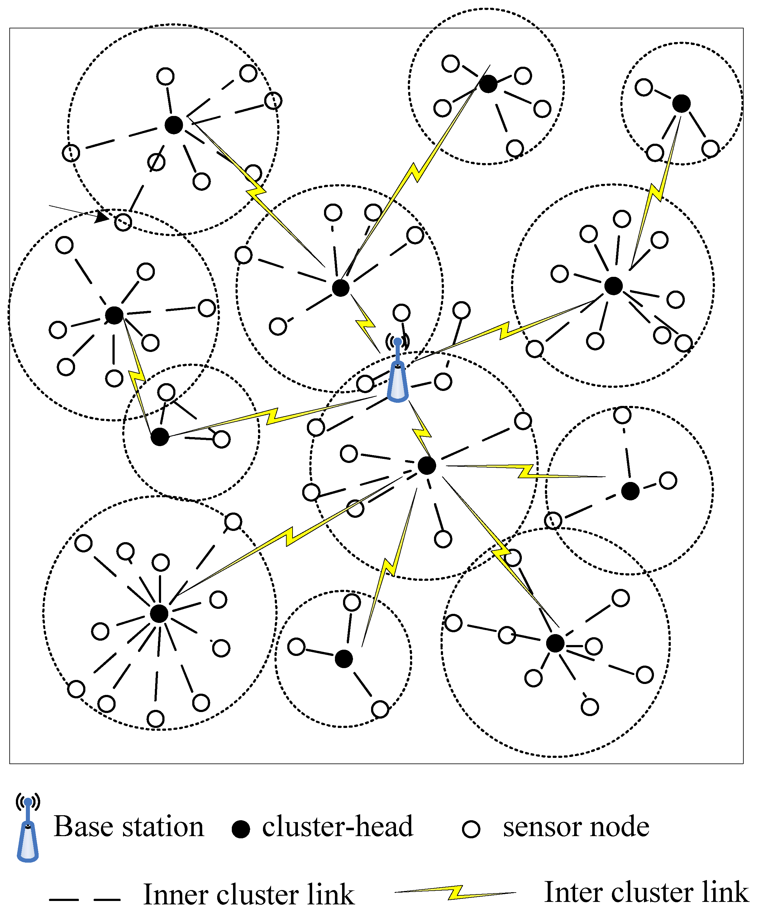
3.1. Network Model

A wireless sensor network scenario is proposed in this paper. It is assumed that N sensor nodes are randomly deployed in a two-dimensional rectangular region of X*Y, and the wireless sensor network is assumed to have the following properties [23,24,25]:

• The network is a static network with a high density, that is, the deployment of sensor nodes remains unchanged, and the node density is sufficient to ensure network connectivity and complete coverage of the monitoring area;
• The base station is fixed and unique and has an unlimited energy supply, and its wireless transmitting power is controllable;
• The sensor nodes are isomorphic and non-rechargeable. The initial energy is the same as E₀;
• The energy consumed by each sensor node is not equal, which makes the network’s energy consumption heterogeneous;
• Nodes have the ability of self-energy perception;
• The nodes can adjust the transmission power [17,25]; and
• The nodes have the ability to fuse data.

3.2. Energy Model

The first-order radio energy consumption model is adopted [26,27], and it is considered that the energy E_tx consumed by the node to send l-bit data is

$$E_{tx}=\{\begin{array}{l}l{E}_{elec}+l{\epsilon }_f{d}^2,d<d_0\\ l{E}_{elec}+l{\epsilon }_m{d}^4,d\ge d_0\end{array}$$

(3)

where E_elec refers to the 1-bit data transmission power of the transmit–receive circuits, d refers to the distance between the transmitter and the receiver, $d_0=\sqrt{\frac{{\epsilon }_f}{{\epsilon }_m}}$ refers to the distance threshold of the model, ${\epsilon }_f$ and ${\epsilon }_m$ refer to the energy coefficients for the power amplification in the two conditions, and l refers to the length of the data packet to be sent.

The energy E_rx that nodes require in order to receive L-bit data can be calculated as follows.

$$E_{rx}=k{E}_{elec}$$

(4)

3.3. Signal Channel Model

Due to the complex environment, there is dense occlusion in the wireless signal’s propagation that will lead to a multi-path effect. This effect produces much uncertainty in the receiving signal’s strength and the link quality. Due to the small-scale effect of multi-path propagation, it can be considered that the signal attenuation of the link between nodes conforms to the following channel model [28,29]:

$$PL=10n\lg d+\mathrm{A}+X$$

(5)

where PL represents the signal attenuation of the link, n is the environmental attenuation coefficient, lg is a base-10 logarithm, d is the distance between transceiver nodes, A is the constant in the model, and X represents the random component of small-scale fading.

A TDMA method is adopted in this paper in order to reduce the interference between nodes. So, the small-scale fading that is caused by environmental noise is considered. For any node N_i, assume that it has k neighbor nodes, NB₁, NB₂,…NB_K, and the link connectivity probabilities are Lqc₁, Lqc₂,…Lqc_m, respectively [30].

$$Lqc=\{\begin{array}{c}1, if (PER=0)\\ {(1-0.5\cdot e^{-\frac{\gamma }{2}\cdot \frac{1}{0.64}})}^{8l}, if (0<PER<1)\\ 0, if (PER=1)\end{array}$$

(6)

where γ is the signal-to-noise ratio (SNR) at the receiving end, PER is the package error rate at the receiving end, and l is the length of the data packet.

Then, the average link quality of node i could be obtained as:

$$Lqc(i)=\frac{1}{m}{\displaystyle \sum _1^{m}Lq{c}_i}$$

(7)

A retransmission scheme is adopted in the network. A packet will be retransmitted when the link quality is poor. In this case, the amount of network transmission data will increase in addition to the network power consumption when the link quality decreases.

4. A Hybrid Routing Algorithm Based on Naïve Bayes and Improved Particle Swarm Optimization Algorithms

A hybrid routing algorithm based on Naïve Bayes and improved particle swarm optimization algorithms (HRA-NP) is proposed in this paper. HRA-NP has the advantages of a simple topology and easy-to-maintain cluster routing. This would improve the energy efficiency of data collection. At the same time, the multi-hop between cluster heads method is adopted to eliminate the energy consumption gradient and energy consumption funnels of remote cluster heads, which makes it more suitable for medium and large-scale network application scenarios [31]. The network diagram of the hybrid routing algorithm is shown in Figure 1.

4.1. Cluster Head Selection Based on a Naïve Bayes Classifier

A Bayesian network can predict the probability of future events through their statistical probability [32,33]. The problem of WSN cluster head selection is to classify local nodes as either cluster head nodes or ordinary nodes. An energy-efficient naïve Bayesian network decision-making method is proposed that estimates the unknown node categories according to the known node categories. By using the Bayes method, the network can be clustered automatically without considering the division of nodes.

Suppose Y⁽ⁱ⁾ is the feature vector of naïve node i, representing a set of features of node naïve, and Y⁽ⁱ⁾ = {Y⁽ⁱ⁾₁, Y⁽ⁱ⁾₂, Y⁽ⁱ⁾₃, … Y⁽ⁱ⁾_k}, where k refers to the dimension of the vector. The features of node i include the residual energy re⁽ⁱ⁾, the distance from the node to the BS ds⁽ⁱ⁾, the node degree de⁽ⁱ⁾, the average distance from the node i to its neighbor dc⁽ⁱ⁾, the average link quality between node i and its neighbor Lqc⁽ⁱ⁾, and the data fusion degree Df⁽ⁱ⁾ when node i becomes the cluster head. The vector can be expressed as follows:

$$Y_{}^{(i)}=\{r{e}^{(i)},d{s}^{(i)},d{e}^{(i)},d{c}^{(i)},Lq{c}^{(i)},D{f}^{(i)}\}$$

(8)

where C represents the category that the node belongs to. In the cluster head selection issue, C is binary, which means that the node is an ordinary node or a cluster head node, expressed as C = {c₀, c₁}. The aim of cluster head selection is to find the mapping relationship between Y⁽ⁱ⁾ and C. Finally, we can obtain P(C|Y⁽ⁱ⁾), which represents the probability of node i becoming the cluster head with the characteristics of Y⁽ⁱ⁾. We can obtain Equation (9) according to the Bayesian theorem.

$$P(C=c_1|Y^{(i)})=\frac{P(Y^{(i)}|C=c_1)P(C=c_1)}{P(Y^{(i)})}$$

(9)

There is an assumption in the Naïve Bayes method that all the features are independent. Then, we can obtain:

$$P(Y^{(i)}|C=c_1)={\displaystyle \prod _i^{K}P(Y_j^{(i)}=y_j|C=c_1)}$$

(10)

Here, we mainly estimate the conditional probability that a node will become a cluster head, so Equation (9) can be transformed into:

$$P(C=c_1|Y_1^{(i)},Y_2^{(i)},\dots Y_k^{(i)})=\frac{P(C=c_1)P(Y_1^{(i)},Y_2^{(i)},\dots Y_k^{(i)}|C=c_1)}{P(Y_1^{(i)},Y_2^{(i)},\dots Y_k^{(i)})}$$

(11)

We select the node with the highest conditional probability of becoming the cluster head within the radius of the clustered domain:

$$C\leftarrow \arg \underset{c_1}{\max }(P(Y^{(i)}|C=c_1))$$

(12)

In a real WSN application, considering that the prior probability estimation caused by the lack of sample data in the training set is 0, the Laplace smoothing method is used for sample estimation.

$$\widehat{P}(C=c_k)=\frac{\#\{C=c_k\}+t}{\#\left\{C\right\}+tK}$$

(13)

where t is the number of false samples added for each class, K is the number of classes, and #{C} represents the number of samples in the training set.

Firstly, the algorithm (Algorithm 1) determines the residual energy of nodes, calculates the probability that all energy-dominant nodes will become cluster heads, selects the node with the greatest probability within the set radius to become the cluster head, and improves the accuracy of cluster head node prediction through sample training. The pseudo code of Algorithm 1 is as follows:

Algorithm 1: Pseudo code for the proposed CH selection method based on a Naïve Bayes classifier.

-Input: The number of sensors N, number of clusters m, and node initial energy E0

-Output: Cluster-head assignment and the cluster partition of all nodes

-Algorithm 1. Network initialization. 2. Randomly generate the initial position of all nodes. Vi = random(x, y) Set the residual energy of all nodes to E0.

3. Calculate re(n),ds(n),de(n),dc(n), and Lqc(n), i.e., the residual energy, distance to the BS, node degree, distance to neighbors, and average link quality. All C(i) = {c0}.

4. For i = 1 to N  Calculate re(i) by using Equations (3) and (4)  Calculate Lqc(i) by using Equations (6) and (7)

5. If re(i) > REThreshold           // Energy advantage node

6.  Add node(i) to Cluster-head Candidate Node Set

7. Else

8.  Add node(i) to Common Perception Node Set

9. End if

10. End for

11. For all nodes in Cluster-head Candidate Node Set

12.  Calculate $P(C=c_1|Y^{(i)})$ by using Equations (9), (11), and (12)  //Probability of becoming CH

13.  Training

14.  If $P(C=c_1|Y^{(i)})$ = max {$P(C=c_1|Y^{(i)})$}

15.    C(i) = {c1}   //set node i as Cluster head

16.  Else

17.    C(i) = {c0}   //set node i as Common Perception Node

18.  End if

19. End for

4.2. Multi-Hop Path Optimization between Cluster Heads Using Improved PSO

Multi-hop path selection between cluster heads in a WSN is a typical combinatorial optimization problem [34,35]. This paper proposes an improved PSO algorithm for multi-hop path selection between cluster heads. By improving the algorithm’s fitness function and initialization method, the search iteration efficiency of the PSO algorithm for the routing path can be improved.

The key element of multi-hop path selection optimization based on the PSO algorithm is the construction of the fitness function [36]. The main goal is to extend the network’s lifetime [37]. During transmission path selection, denote a multi-hop path from the source node to the BS as PT_i, which refers to a particle in the PSO algorithm.

$$Fitness\propto \frac{1}{{\displaystyle \sum _{PT}\frac{E{r}_i}{E{r}_{average}{}_i}}}$$

(14)

where Er_average is the average node residual energy of the network and Er_i is the residual energy of node i.

Similarly, it is desirable to select the path with the lowest expected energy consumption Ec

$$Fitness\propto \frac{1}{Ec}$$

(15)

Equations (13) and (14) represent the energy factor in the definition of the fitness function, that is, the optimal path should satisfy the condition that the path energy depletion should be as small as possible and the relative residual energy of nodes on the path should be as high as possible.

In addition, the number of hops has a significant impact on the efficiency of the routing algorithm and the network energy consumption performance [38]. Therefore, the number of hops should be as small as possible when solving for the optimal path. In addition, due to the signal fading characteristics under conditions of complex dynamics, we take the link quality as one of the parameters of the fitness function and give priority to the link with the highest quality as the multi-hop path. Then, we can obtain:

$$Fitness\propto \frac{1}{\mathrm{H}ops}$$

(16)

$$Fitness\propto {\displaystyle \sum _{PT}\frac{1}{Lqc}}$$

(17)

Combining Equations (14)–(17), we can obtain:

$$Fitness=\frac{w{\displaystyle \sum _{PT}\frac{1}{Lqc}}}{Ec\times Hops\times {\displaystyle \sum _{PT}\frac{E{r}_i}{E{r}_{average}{}_i}}}$$

(18)

where w is the weight factor. The algorithm calculates the individual optimal position and the global optimal position according to the initial position and speed and starts iterative optimization. The particle velocity update method is shown in Equation (19).

$$\{\begin{array}{c}{v}_{xid}(t)=\omega v_{xid}(t-1)+c_1{r}_1(p_{xid}(t-1)-x_{xid}(t-1))+c_2{r}_2(p_{xgd}(t-1)-x_{xid}(t-1))\\ v_{yid}(t)=\omega v_{yid}(t-1)+c_1{r}_1(p_{yid}(t-1)-x_{yid}(t-1))+c_2{r}_2(p_{ygd}(t-1)-x_{yid}(t-1))\end{array}$$

(19)

where ω are inertia factors, c₁ and c₂ are learning factors, and r₁ and r₂ are random numbers between 0 and 1 that can make the particle mutation have a certain degree of randomness and help it to avoid falling into the local optimum. The particle position update method is shown in Equation (20).

$$\{\begin{array}{c}{x}_{xid}(t)=x_{xid}(t-1)+v_{xid}(t)\\ x_{yid}(t)=x_{yid}(t-1)+v_{yid}(t)\end{array}$$

(20)

After the cluster head node is selected, the particle position and speed in the algorithm are initialized, and the fitness function is constructed by the node energy consumption, residual energy, minimum number of hops, distance from the BS, and link quality. The particle swarm optimization algorithm is used to determine the optimal routing path in accordance with the complex dynamic environment of farmland. The specific steps of the algorithm (Algorithm 2) are as follows:

• Establish the initial path PT_i from each cluster head to the BS and the initial position and speed of the corresponding particle;
• Calculate the fitness function value of each path according to Equation (18);
• Calculate the individual extreme value, global extreme value, particle position, and velocity update value according to Equations (19) and (20);
• Repeat Step 2 to Step 3 until the individual extreme value converges to the global extreme value or the algorithm reaches the maximum number of iterations; and
• Start multi-hop transmission according to the obtained optimal routing path, obtain node energy and link quality data at the same time, and update the routing path during the next data transmission.

The pseudo code of Algorithm 2 is as follows:

Algorithm 2: Pseudo code for the proposed multi-hop routing method based on an improved PSO algorithm.

-Input: The number of clusters m, position of all cluster heads (Xi, Yi), residual energy of all cluster heads Eri, number of iterations Niter, object weight w, inertia factor ω, and learning factors c1 and c2

-Output: Optimized multi-hop routing path of all cluster heads

-Algorithm 1. After cluster head selection and inner cluster data collection 2. Calculate Eraverage, Hops, and Lqc(n), i.e., the average residual energy, number of hops to the BS, node degree, and link quality.

3. Find all possible paths from each cluster head to the BS PT{ }

4. Particle initialization

5. for all PTi∈PT{ }

6. Calculate Fitness(PTi) using Equation (18)

7. Calculate the individual extremum, global extremum, particle position, and velocity update values using Equations (19) and (20) // Particle swarm update iteration

8. If the individual extremum reaches the global extremum     // Algorithm convergence

9.  Break;

10. Else if

11.  Number of iterations ≥ Niter        // Maximum number of iterations reached

12.  Break;

13. Else

14. go to step 6.

15. end for

5. Experimental Results and Analysis

5.1. Experiment Setting

The simulations were performed in an area with a size of 400 × 400 m². A total of 200 sensor nodes were deployed randomly, and their positions remained constant over all the experiments. The simulations were carried out in MATLAB R2019. The proposed HRA-NP algorithm was compared with ECRRS [17], FC-RBAT [22], and DUCF [25]. All other parameters used in the simulations are presented in

Table 1. Parameter settings in the simulation.

Parameters	Value
Area size	400 × 400 m2
Node number N	200
The position of the base station	(200, 200)
Node initial energy E0	5 J
Inner cluster communication range Tmax	100 m
εm	0.001 pJ·b−1
εf	10 pJ·b−1·m−2
Eelec	50 nJ·b−1
Packet size	4000 bits
Control message size	400 bits
Maximum iteration number for PSO	500
Inertia factor ω	0.797
Learning factor c1, c2	1.497

[1,5,17,39,40,41].

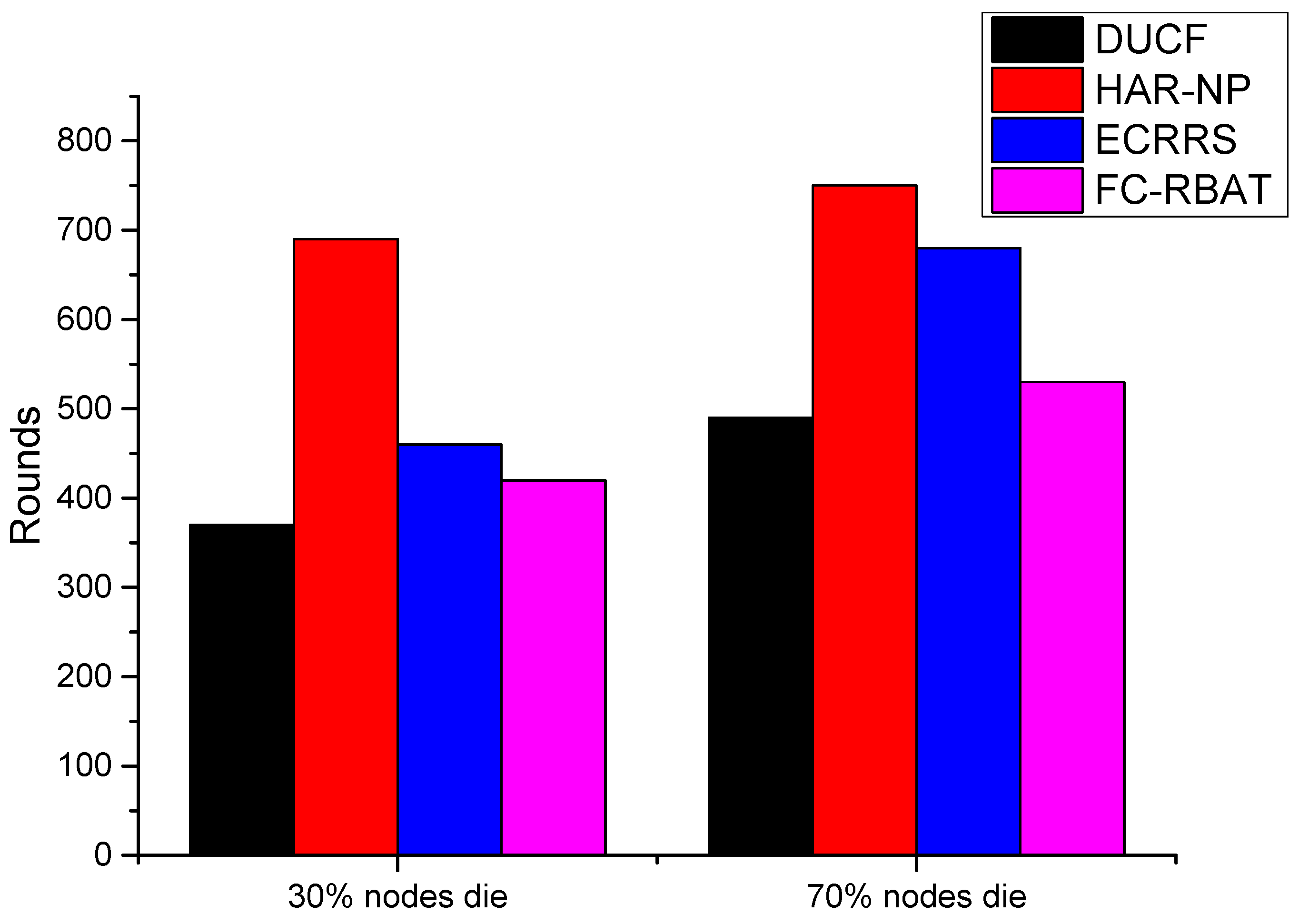
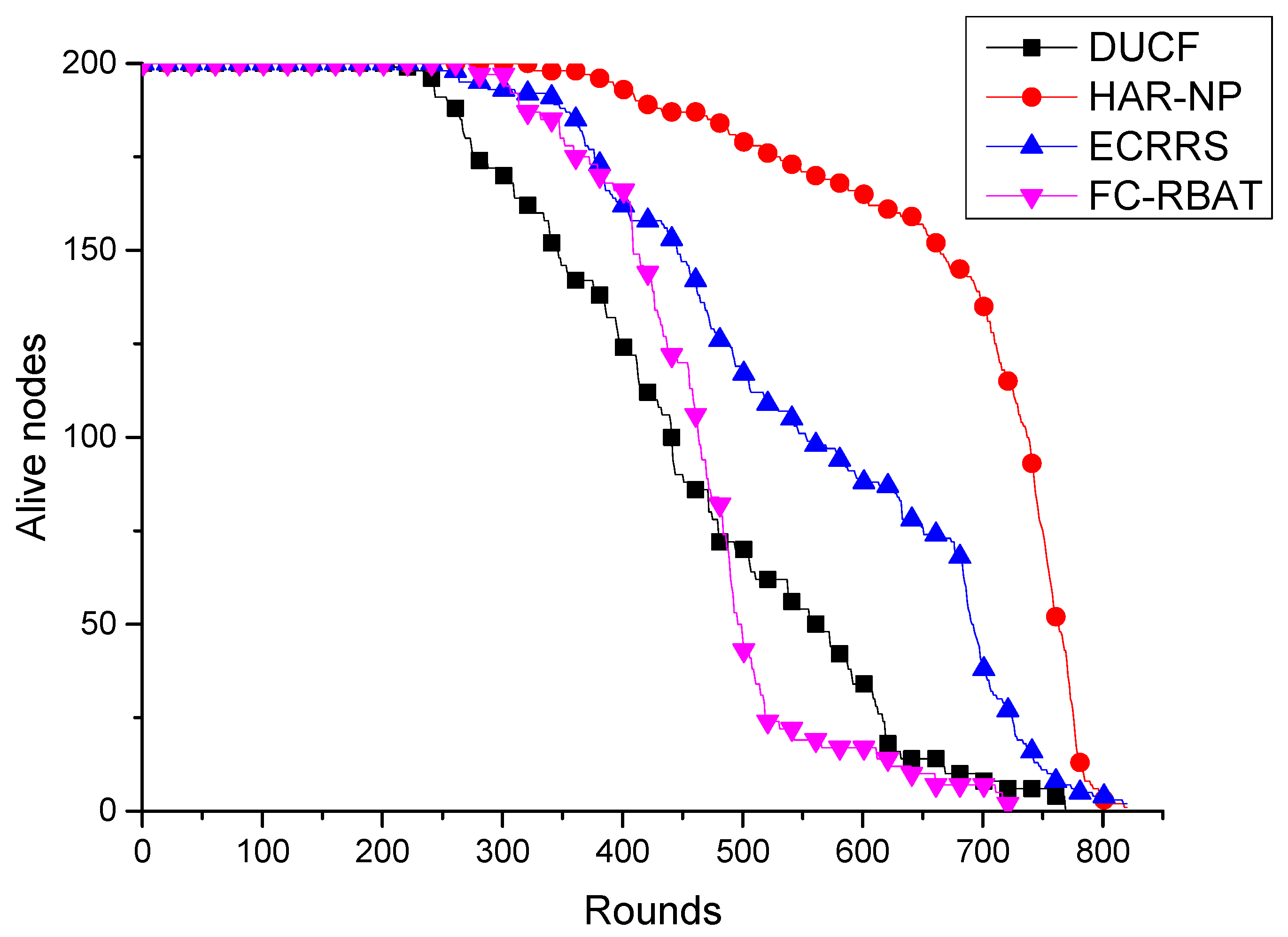
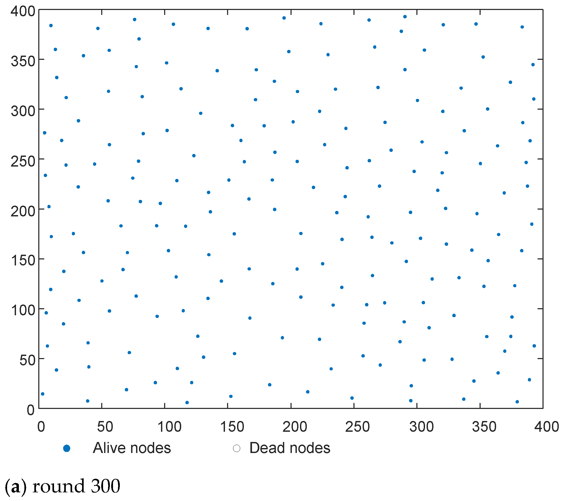
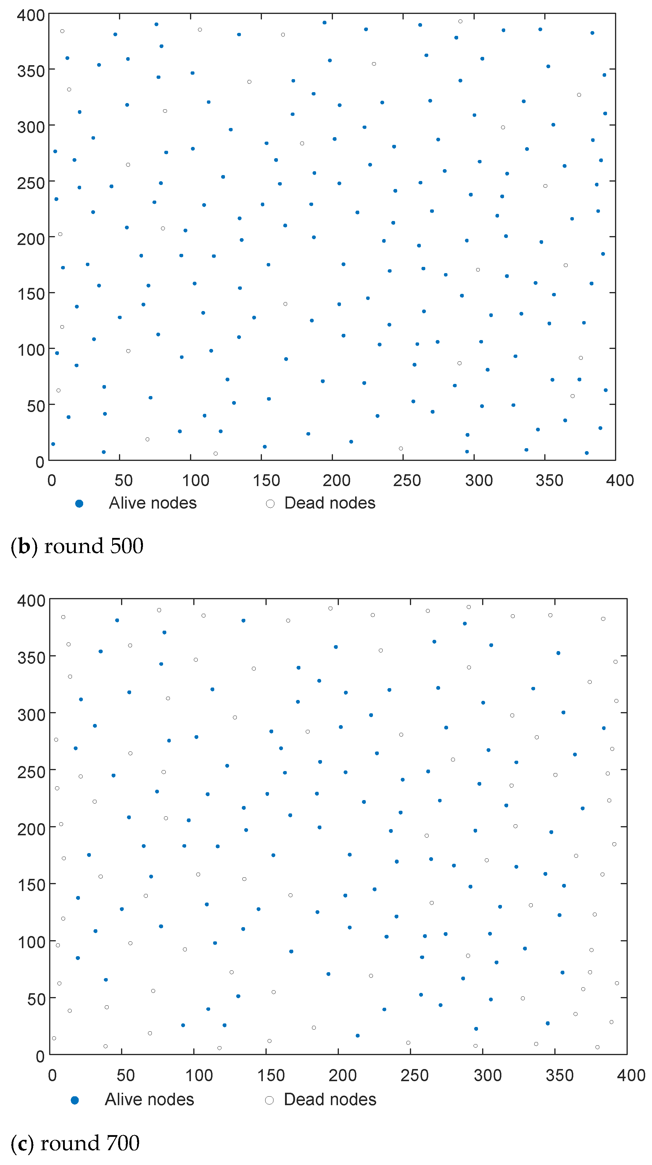
5.2. Network Life Cycle and Number of Alive Nodes

Nodes with less than zero residual energy were considered dead nodes because they cannot perform any activities without energy. Figure 2 shows the number of alive nodes per round for the four algorithms. When the network runs to about 200 rounds, the first dead node appears in the DUCF algorithm. The first dead node in the ECRRS and FC-RBAT algorithms appears at about 230 and 260 rounds, respectively. The first dead node in the HRA-NP algorithm appears at about 310 rounds. The death time of all nodes in FC-RBAT is about 710 rounds, that in DUCF is about 770 rounds, and that in ECRRS and HRA-NP is about 810 rounds. As can be seen, the network lifetime of FC-RBAT and DUCF is almost the same, and there are differences in the speed at which nodes die in different stages. In the early stage of the network, the node death rate of FC-RBAT is slower than that of DUCF. At about 400 rounds, the node death rate of FC-RBAT increases. At about 480 rounds, the number of dead nodes in FC-RBAT exceeds that in DUCF. The network lifetime of ECRRS is slightly longer than that of the other two algorithms, and the network lifetime of the HAR-NP algorithm is the longest. The ECRRS and HAR-NP algorithms have a low rate of node mortality, and the number of node deaths increases rapidly until the network ends.

From the perspective of network data transmission, the death time of the first dead node and all nodes cannot well represent the survival cycle of the network function. Because of its self-organizing characteristics, the network’s performance will not be significantly affected when a small number of nodes die. It is generally believed that when the proportion of dead nodes reaches more than 30%, the network transmission performance begins to have a significant impact. When the proportion of dead nodes reaches more than 70%, the network structure is damaged and basically loses its ability to function. Therefore, the 30% node and 70% node death times have more practical reference value for network monitoring applications.

As is shown in Figure 3, DUCF, FC-RBAT, ECRRS, and HRA-NP had 30% node death times of 370, 420, 460, and 690 rounds, respectively, and 70% of the nodes died in 490, 530, 680, and 750 rounds, respectively. Although there is little difference between the death time of the first node and that of all nodes, it can be seen from Figure 3 that the 30% node death time of HRA-NP is 1.87 times, 1.64 times, and 1.5 times that of DUCF, FC-RBAT, and ECRRS, respectively. The 70% node death time of HRA-NP is 1.53 times, 1.41 times, and 1.1 times that of DUCF, FC-RBAT, and ECRRS, respectively. This shows that the HRA-NP protocol has obvious performance advantages in the actual effective life cycle of the network. The possible reason for this is that the HRA-NP algorithm optimizes the clustering efficiency and the cluster head multi-hop transmission path, reduces and balances the node energy consumption, and effectively prolongs the network lifetime.

The distribution of alive and dead nodes in HAR-NP is shown in Figure 4. Figure 4a–c show the distribution at round 300, 500, and 700, respectively. There are more dead nodes at the edge of the network at round 500. At round 700, dead nodes appear in most areas of the network, except for the area within one-hop distance to the BS. The distribution of alive nodes shows that the algorithm has good energy balance performance.

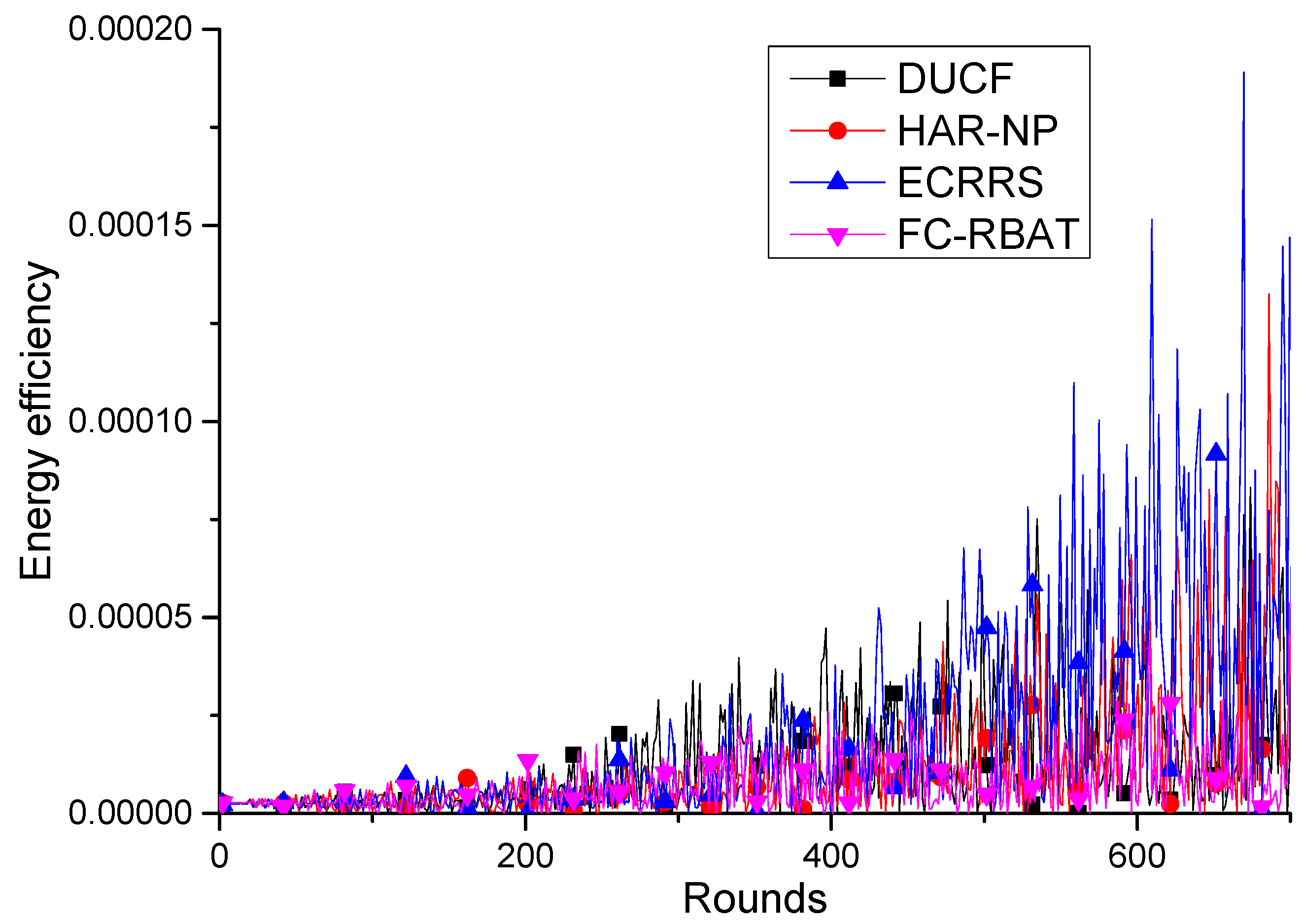
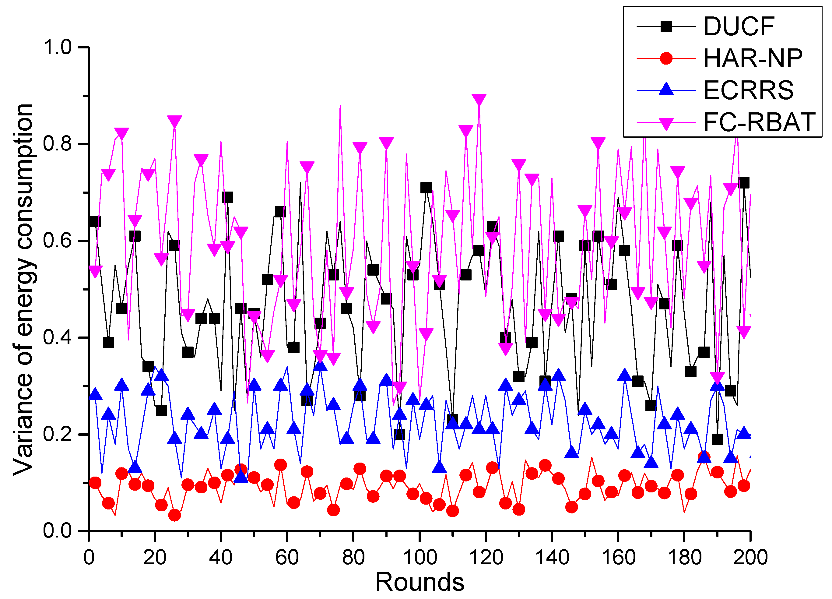
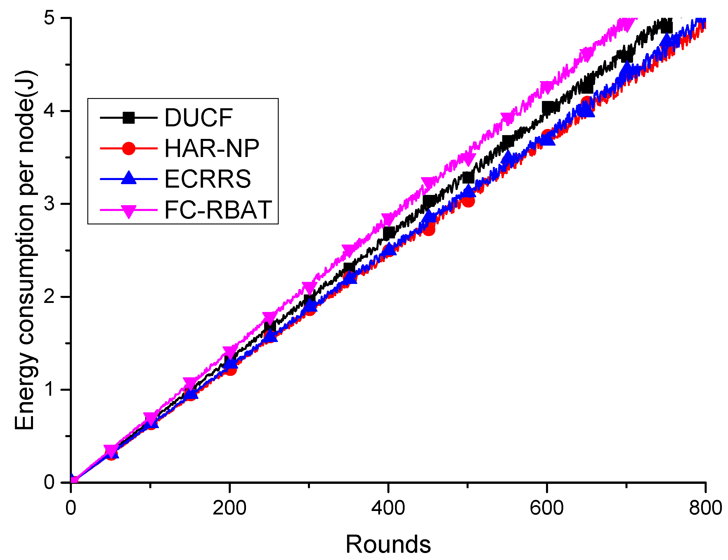
5.3. Node Energy Consumption

The average energy consumption of network nodes is shown in Figure 5. The average energy consumption curves of the network nodes of the four algorithms are approximately straight lines as a whole, and the order of slopes (from most steep to least steep) is FC-RBAT, DUCF, ECRRS, and HRA-NP. It can be seen from Figure 5 that the average energy consumption of network nodes remains stable, which is mainly determined by the deployment location of network nodes. According to the different algorithms, the average energy consumption of nodes varies to a certain extent. It should be noted that it takes time to calculate the average energy consumption of network nodes, and dead nodes are not included in the calculation. Therefore, what is shown in Figure 5 is mainly a comparison of the average energy consumption levels of nodes between the different algorithms and does not reflect the energy consumption balance performance between nodes.

The network node energy consumption efficiency E_effi is defined as the average node energy consumption per round Ec_r divided by the current round of data transmission dt_tp, which can be considered as the amount of energy consumed when transmitting 1 bit of data, i.e.,

$$E_{effi}=\frac{E{c}_r}{d{t}_{tp}}$$

(21)

It is easy to find from the definition of E_effi that the larger the E_effi value, the lower the energy utilization rate of network nodes. In contrast, the smaller the E_effi value, the higher the energy utilization rate of network nodes.

As can be seen from Figure 6, the energy consumption efficiency of the network nodes of the four algorithms maintains a low level before 200 rounds and then gradually increases after 200 rounds. As the number of rounds increases, the energy consumption efficiency curves diverge. At about 600 rounds, ECRRS has the largest energy efficiency value, DUCF and HAR-NP are in the middle, and FC-RBAT has the smallest energy efficiency value. As is shown in the figure, all four algorithms have a good energy utilization rate before 200 rounds. After 200 rounds, as the number of dead nodes increases, the network structure is affected, and the energy utilization rate decreases. After 600 rounds, about 70% of the nodes die, the overall network structure is damaged, and the energy consumption efficiency curve is in a divergent state.

The variation in the energy consumption of network nodes is an important index for measuring the energy consumption balance performance of routing algorithms. As can be seen in Figure 6, the death of network nodes has a great impact on the energy consumption distribution of the network. Therefore, we compared the energy consumption variance of network nodes of the four algorithms from round 0 to round 200 as shown in Figure 7. The energy consumption variance of the HRA-NP algorithm is the smallest, followed by ECRRS. The energy consumption variance of the DUCF and FC-RBAT algorithms is the largest, indicating that the average energy consumption difference of each round for the HRA-NP algorithm is small. In the HRA-NP algorithm, cluster heads are selected based on the distance from the node to the BS, the node degree, the average distance in the cluster, and the average link quality in the cluster. At the same time, the energy consumption cost of multi-hop paths between cluster heads is estimated to ensure that the algorithm has good energy consumption balance performance.

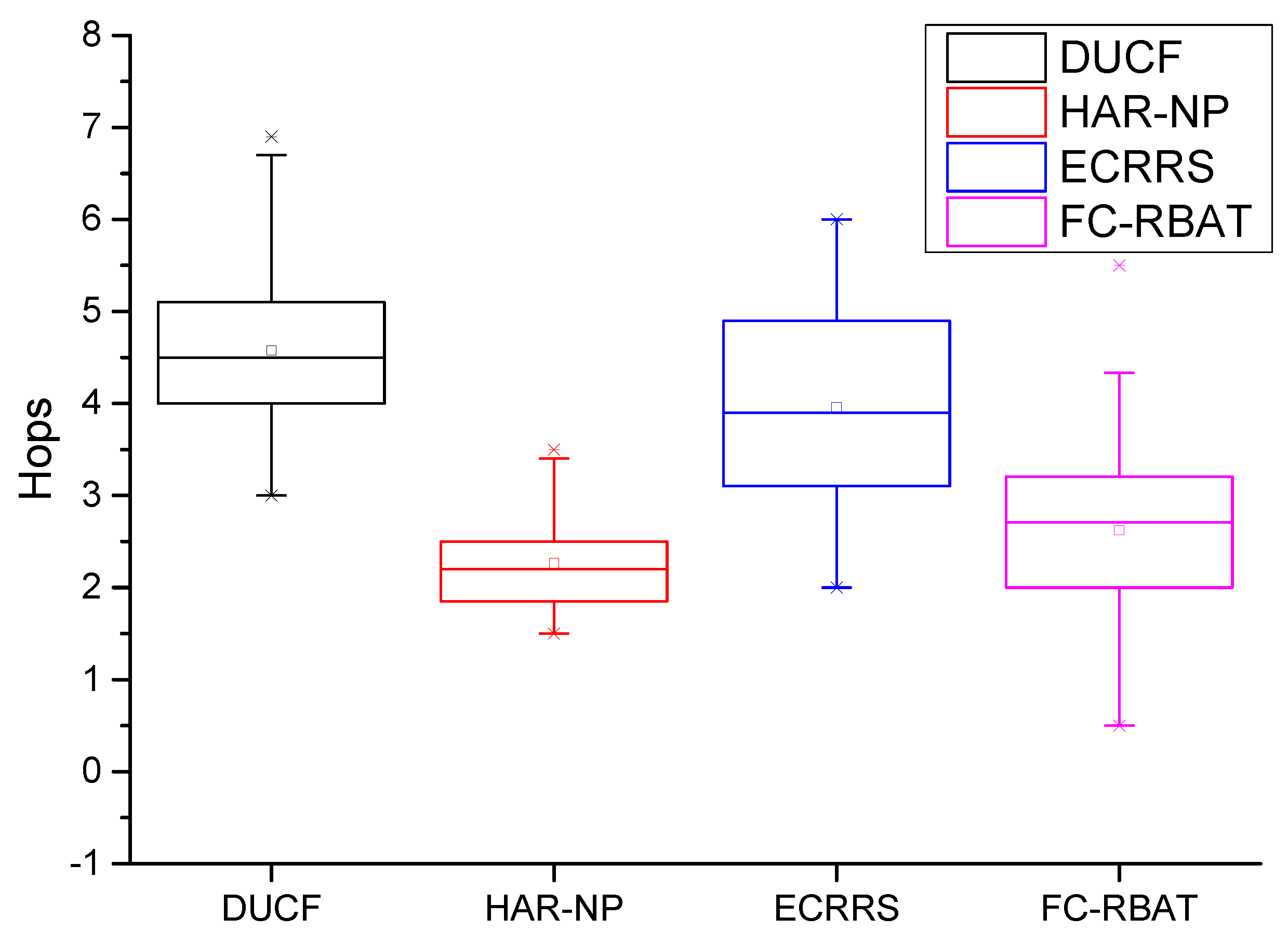
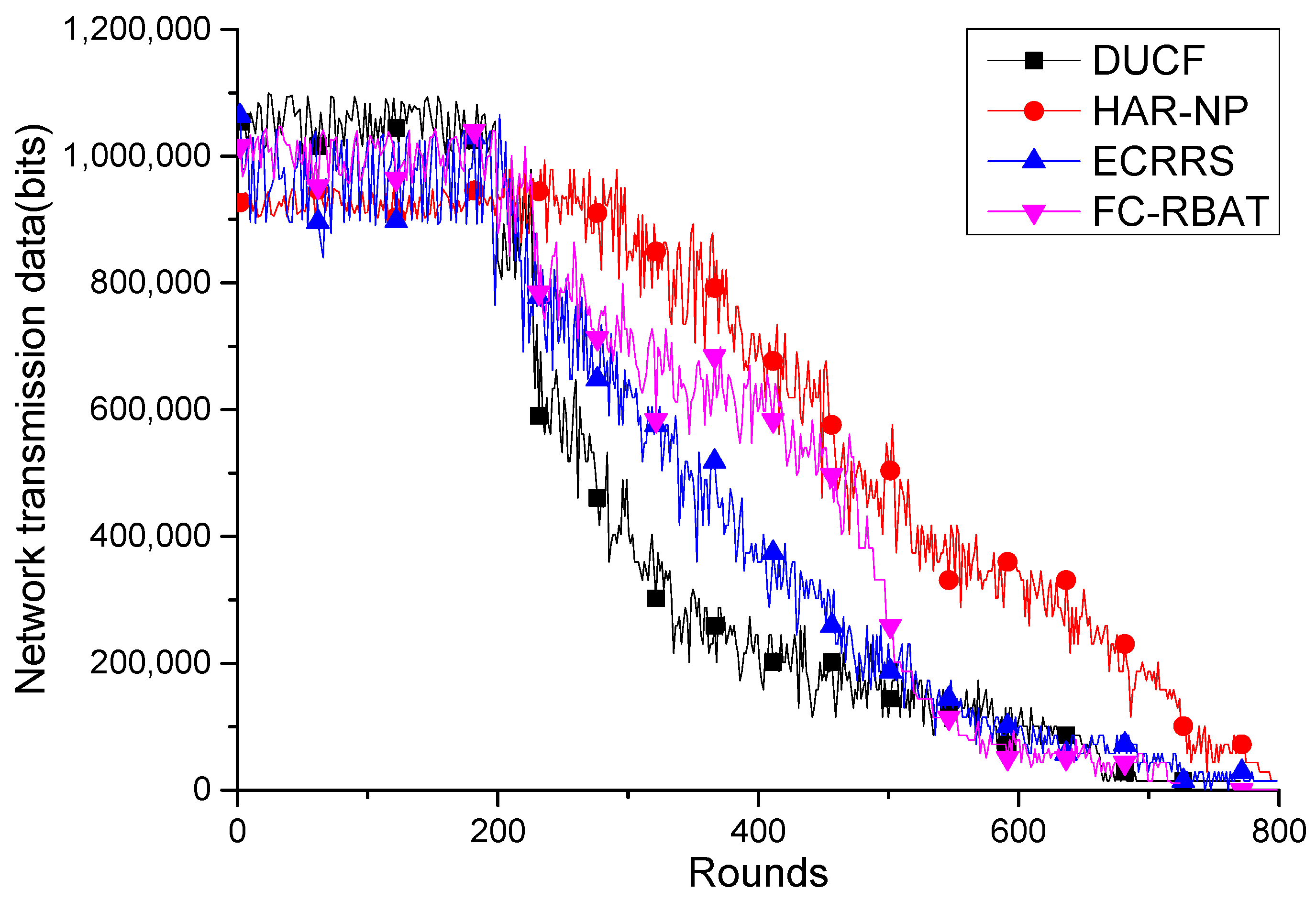
5.4. Average Number of Hops and Network Data Throughput

The average number of hops in the network is shown in Figure 8. From the average and maximum numbers of hops, the order (from large to small) of the four algorithms is DUCF, ECRRS, FC-RBAT, and HRA-NP, and the average number of hops is 4.5, 4.0, 2.8, and 2.3, respectively. In terms of the minimum number of hops, the order (from large to small) is DUCF, ECRRS, HRA-NP, and FC-RBAT. On the whole, the DUCF algorithm has the highest average number of hops, HRA-NP has the lowest average number of hops, and the ECRRS and FC-RBAT algorithms are in the middle, with the FC-RBAT algorithm having a slightly larger number of average hopes than the ECRRS algorithm.

Network transmission data is also an important performance parameter in routing algorithms. Network transmission data is the total number of bits transmitted per round. In Figure 8, it can be seen that in the early stage of the network’s operation, the network transmission data and stability are around 1 × 10⁶ bits. HAR-NP has the lowest value, followed by ECRRS. The DUCF and FC-RBAT algorithms have slightly higher values. As the amount of surviving node data in the network decreases, the total network data energy shows an overall downward trend, which is basically consistent with the decreasing trend of the node data. Moreover, during rounds 260 to 700, the network transmission data curve of the HAR-NP algorithm is closer to those of the other three algorithms than to the survival node curve. This is because, when using the Naïve Bayes method for clustering, the degree of data fusion in the cluster is taken as one of the weights. Through data fusion in the cluster, the amount of data transmitted and energy consumed is effectively reduced.

There are some differences between the transmission data curve (Figure 9) and the alive node curve (Figure 2). The transmission data curves of the HAR-NP and FC-RBAT algorithms shown in Figure 9 seem to be lower than those shown in Figure 2 compared with the DUCF and ECRRS algorithms. This is mainly because of the different average numbers of hops in the four algorithms as shown in Figure 8. Thus, HAR-NP and FC-RBAT would have fewer transmission bits than the other two algorithms. Moreover, the clustering’s organization may also have an impact on the data transmission performance because of the data fusion in the cluster head.

6. Conclusions

Aiming at the requirement of high-energy-efficiency WSN monitoring in a noisy environment, a hybrid routing algorithm based on Naïve Bayes and improved particle swarm optimization algorithms is proposed. In HRA-NP, the sensor nodes are grouped together to form balanced clusters using the Naïve Bayes algorithm. After the clusters are formed, a CH from each cluster is selected according to the CH conditional probability of the sensor nodes. The score of the sensor node is defined using four factors (residual energy, distance from the BS, distance from the cluster’s center, and intra-cluster distance). Therefore, energy balancing can be implemented in the WSN. Furthermore, the best multi-hop path between cluster heads is determined according to an improved PSO approach. A novel fitness function was designed to evaluate the solutions generated by the PSO approach. The fittest solution provides information about the best routing path towards the BS. Simulations were carried out on various evaluation factors, and HRA-NP was found to outperform DUCF, ECRRS, and FC-RBAT in terms of the evaluation factors. Possible future research direction include consideration of end-to-end delay and other features that affect the algorithm’s performance. A mobile sink is also a prospective way to improve the network performance.

References

1. Rostami, A.S.; Badkoobe, M.; Mohanna, F.; Hosseinabadi, A.A.R.; Sangaiah, A.K. Survey on clustering in heterogeneous and homogeneous wireless sensor networks. J. Supercomput. 2018, 74, 277–323. [Google Scholar] [CrossRef]
2. Sundararaj, V.; Muthukumar, S.; Kumar, R.S. An optimal cluster formation based energy efficient dynamic scheduling hybrid MAC protocol for heavy traffic load in wireless sensor networks. Comput. Secur. 2018, 77, 277–288. [Google Scholar] [CrossRef]
3. Hassan, A.; Alshomrani, S.; Altalhi, A.; Ahsan, S. Improved routing metrics for energy constrained interconnected devices in low-power and lossy networks. J. Commun. Netw. 2016, 18, 327–332. [Google Scholar] [CrossRef]
4. Panchal, A.; Singh, R.K. EADCR: Energy Aware Distance Based Cluster Head Selection and Routing Protocol for Wireless Sensor Networks. J. Circuits Syst. Comput. 2020, 30, 2150063. [Google Scholar] [CrossRef]
5. Kumar, N.; Singh, Y. An energy efficient and trust management based opportunistic routing metric for wireless sensor networks. In Proceedings of the 2016 Fourth International Conference on Parallel, Distributed and Grid Computing, Waknaghat, India, 22–24 December 2016; pp. 611–616. [Google Scholar] [CrossRef]
6. Mohamad, M.M.; Kheirabadi, M.T. Energy efficient opportunistic routing algorithm for underwater sensor network: A review. In Proceedings of the 2016 2nd International Conference on Science in Information Technology, Balikpapan, Indonesia, 26–27 October 2016; pp. 41–46. [Google Scholar] [CrossRef]
7. Rajeswari, A.R.; Kulothungan, K.; Ganapathy, S.; Kannan, A. Trusted energy aware cluster based routing using fuzzy logic for WSN in IoT. J. Intell. Fuzzy Syst. 2021, 40, 9197–9211. [Google Scholar] [CrossRef]
8. Choudhary, A.; Kumar, S.; Gupta, S.; Gong, M.; Mahanti, A. FEHCA: A Fault-Tolerant Energy-Efficient Hierarchical Clustering Algorithm for Wireless Sensor Networks. Energies 2021, 14, 3935. [Google Scholar] [CrossRef]
9. Sadrishojaei, M.; Navimipour, N.J.; Reshadi, M.; Hosseinzadeh, M. A new clustering-based routing method in the mobile internet of things using a krill herd algorithm. Clust. Comput. -J. Netw. Softw. Tools Appl. 2021, 25, 351–361. Available online: https://link.springer.com/article/10.1007%2Fs10586-021-03394-1 (accessed on 11 November 2021). [CrossRef]
10. Manuel, A.J.; Deverajan, G.G.; Patan, R.; Gandomi, A.H. Optimization of Routing-Based Clustering Approaches in Wireless Sensor Network: Review and Open Research Issues. Electronics 2020, 9, 1630. [Google Scholar] [CrossRef]
11. Handy, M.J.; Haase, M.; Timmermann, D. Low energy adaptive clustering hierarchy with deterministic cluster-head selection. In Proceedings of the 2002 4th International Workshop on Mobile and Wireless Communications Network, Stockholm, Sweden, 9–11 September 2002; pp. 368–372. [Google Scholar] [CrossRef]
12. Al-Shalabi, M.; Anbar, M.; Wan, T.C.; Khasawneh, A. Variants of the Low-Energy Adaptive Clustering Hierarchy Protocol: Survey, Issues and Challenges. Electronics 2018, 7, 136. [Google Scholar] [CrossRef] [Green Version]
13. Wu, H.R.; Zhao, C.J.; Zhang, H.H. Cluster head cycle-switching schemes for farmland wireless sensor networks. Trans. Chin. Soc. Agric. Eng. 2009, 25, 170–174. [Google Scholar] [CrossRef]
14. Gattani, V.S.; Jafri, S.M.H. Data collection using score based load balancing algorithm in wireless sensor networks. In Proceedings of the 2016 2nd International Conference on Science in Information Technology (ICSITech), Balikpapan, Indonesia, 26–27 October 2016; pp. 41–46. [Google Scholar] [CrossRef]
15. Huang, B.W.; Wang, B.; Ding, J.; Gao, R. A Routing Protocol of Wireless Sensor Networks Based on K-Center. Comput. Sci. Appl. 2019, 9, 495–500. [Google Scholar] [CrossRef]
16. Ye, M.; Li, C.F.; Chen, G.H.; Wu, J. EECS: An energy efficient clustering scheme in wireless sensor networks. In Proceedings of the 24th IEEE International Performance, Computing, and Communications Conference, Phoenix, AZ, USA, 7–9 April 2005; pp. 535–540. [Google Scholar] [CrossRef]
17. Wu, H.R.; Zhu, H.J.; Miao, Y.S. An Energy Efficient Cluster-Head Rotation and Relay Node Selection Scheme for Farmland Heterogeneous Wireless Sensor Networks. Wirel. Pers. Commun. 2018, 101, 1639–1655. [Google Scholar] [CrossRef]
18. Sun, X.; Wu, B.G.; Wu, H.R.; Miao, Y.S. Topology Based Energy Efficient Routing Algorithm in Farmland Wireless Sensor Network. Trans. Chin. Soc. Agric. Mach. 2015, 46, 232–238. [Google Scholar]
19. Mhatre, V.; Rosenberg, C. Design guidelines for wireless sensor networks: Communication, clustering and aggregation. Ad Hoc Netw. 2004, 2, 45–63. [Google Scholar] [CrossRef] [Green Version]
20. Rogers, A.; David, E.; Jennings, N.R. Self-organized routing for wireless microsensor networks. IEEE Trans. Syst. Man Cybern.-Part A Syst. Hum. 2005, 35, 349–359. [Google Scholar] [CrossRef]
21. Li, H.; Liu, Z.W.; Guo, Y.Y. Low Energy Routing Protocol Combined with Near Source Data Aggregation and Congestion Control in WSN. J. Chongqing Univ. Technol. (Nat. Sci.) 2019, 33, 111–120. [Google Scholar]
22. Lipare, A.; Edla, D.R.; Dharavath, R. Energy efficient fuzzy clustering and routing using BAT algorithm. Wirel. Netw. 2021, 27, 2813–2828. [Google Scholar] [CrossRef]
23. Miao, Y.S.; Zhao, C.J.; Wu, H.R. Non-uniform clustering routing protocol of wheat farmland based on effective energy consumption. Int. J. Agric. Biol. Eng. 2021, 14, 142–150. [Google Scholar] [CrossRef]
24. Anisi, M.H.; Abdul-Salaam, G.; Abdullah, A.H. A survey of wireless sensor network approaches and their energy consumption for monitoring farm fields in precision agriculture. Precis. Agric. 2015, 16, 216–238. [Google Scholar] [CrossRef]
25. Baranidharan, B.; Santhi, B. DUCF: Distributed load balancing unequal clustering in wireless sensor networks using fuzzy approach. Appl. Soft Comput. 2016, 40, 495–506. [Google Scholar] [CrossRef]
26. Zhao, M.; Chong, P.H.J.; Chan, H.C.B. An Energy-Efficient and Cluster-parent based RPL with Power-level Refinement for Low-Power and Lossy Networks. Comput. Commun. 2017, 104, 17–33. [Google Scholar] [CrossRef]
27. Logambigai, R.; Ganapathy, S.; Kannan, A. Energy–efficient grid–based routing algorithm using intelligent fuzzy rules for wireless sensor networks. Comput. Electr. Eng. 2018, 68, 62–75. [Google Scholar] [CrossRef]
28. Sobral, J.; Rodrigues, J.; Rabelo, R.; Al-Muhtadi, J. Routing Protocols for Low Power and Lossy Networks in Internet of Things Applications. Sensors 2019, 19, 2144. [Google Scholar] [CrossRef] [PubMed] [Green Version]
29. Murali, S.; Jamalipour, A. Mobility-Aware Energy-Efficient Parent Selection Algorithm for Low Power and Lossy Networks. IEEE Internet Things J. 2019, 6, 2593–2601. [Google Scholar] [CrossRef]
30. Hu, H.F.; Yang, Z. Collaborative opportunistic routing in wireless sensor networks. J. Commun. 2009, 30, 116–120. [Google Scholar] [CrossRef]
31. Raval, G.; Bhavsar, M.; Patel, N. Enhancing data delivery with density controlled clustering in wireless sensor networks. Microsyst. Technol. 2017, 23, 613–631. [Google Scholar] [CrossRef]
32. Yuen, K.V.; Kuok, S.C. Efficient Bayesian sensor placement algorithm for structural identification: A general approach for multi-type sensory systems. Earthq. Eng. Struct. Dyn. 2015, 44, 757–774. [Google Scholar] [CrossRef]
33. Jafarizadeh, V.; Keshavarzi, A.; Derikvand, T. Efficient cluster head selection using Naïve Bayes classifier for wireless sensor networks. Wirel. Netw. 2016, 23, 779–785. [Google Scholar] [CrossRef]
34. Jiang, R.; Xiong, K.; Zhang, Y.; Zhou, L.; Liu, T.; Zhong, Z. Outage and Throughput of WPCN-SWIPT Networks with Nonlinear EH Model in Nakagami-m Fading. Electronics 2019, 8, 138. [Google Scholar] [CrossRef] [Green Version]
35. Shah, Z.; Levula, A.; Khurshid, K.; Ahmed, J.; Ullah, I.; Singh, S. Routing Protocols for Mobile Internet of Things (IoT): A Survey on Challenges and Solutions. Electronics 2021, 10, 2320. [Google Scholar] [CrossRef]
36. Yu, X.H.; Zhang, J.; Tao, T.; Gong, L.B.; Huang, Y.M.; Fu, T.W. An energy consumption balanced clustering algorithm for wireless sensor networks based on ant colony strategy. Comput. Eng. Sci. 2019, 41, 1197–1202. [Google Scholar]
37. Liu, J.; Ouyang, H.; Han, X.; Liu, G.R. Optimal sensor placement for uncertain inverse problem of structural parameter estimation. Mech. Syst. Signal Process. 2021, 160, 107914. [Google Scholar] [CrossRef]
38. Gul, M.; Catbas, F.N. Structural health monitoring and damage assessment using a novel time series analysis methodology with sensor clustering. J. Sound Vib. 2011, 330, 1196–1210. [Google Scholar] [CrossRef]
39. Hanafi, E. MBMQA: A Multicriteria-Aware Routing Approach for the IoT 5G Network Based on D2D Communication. Electronics 2021, 10, 2937. [Google Scholar] [CrossRef]
40. Urmonov, O.; Kim, H.W. An Energy-Efficient Fail Recovery Routing in TDMA MAC Protocol-Based Wireless Sensor Network. Electronics 2018, 7, 444. [Google Scholar] [CrossRef] [Green Version]
41. Wang, H.; Roman, H.E.; Yuan, L.Y.; Huang, Y.F.; Wang, R.L. Connectivity, coverage and power consumption in large-scale wireless sensor networks. Comput. Netw. 2014, 75, 212–225. [Google Scholar] [CrossRef]
Figure 1. Network architecture of the WSN hybrid routing algorithm.
Electronics 11 00869 g001
Figure 2. Comparison of the number of alive nodes.
Electronics 11 00869 g002
Figure 3. Comparison of the 30% and 70% node death times of the four algorithms.
Electronics 11 00869 g003
Figure 4. Node distribution of HAR-NP in different rounds.
Electronics 11 00869 g004aElectronics 11 00869 g004b
Figure 5. Average energy consumption of network nodes.
Electronics 11 00869 g005
Figure 6. Comparison of network energy efficiency.
Electronics 11 00869 g006
Figure 7. Comparison of the energy consumption variance of network nodes.
Electronics 11 00869 g007
Figure 8. Comparison of the average number of network hops.
Electronics 11 00869 g008
Figure 9. Comparison of network transmission data.
Electronics 11 00869 g009