
Improved Multiple Vector Representations of Images and Robust Dictionary Learning


Abstract
:1. Introduction
- (1)
- A robust dictionary learning method based on image multi-vector representation is proposed.
- (2)
- A novel representation of images is designed, which is represented by virtual samples and multi-vectors. Based on the original algorithm, four new vector representation methods are added to better mine the large-scale information and global features of images.
- (3)
- A reasonable weighted fusion image classification algorithm is proposed. The influence factor is introduced to automatically adjust the weight of each classifier in the final decision results, which has a significant effect on better extracting image features and can obtain very stable and accurate classification results.
2. Proposed Method
2.1. To Obtain Novel Representations of Images
- (1)
- Generate a virtual image V from the original image I. The representation method of generating V is as follows:
- (2)
- Convert I and V into an improved multi-vector representation of the image.
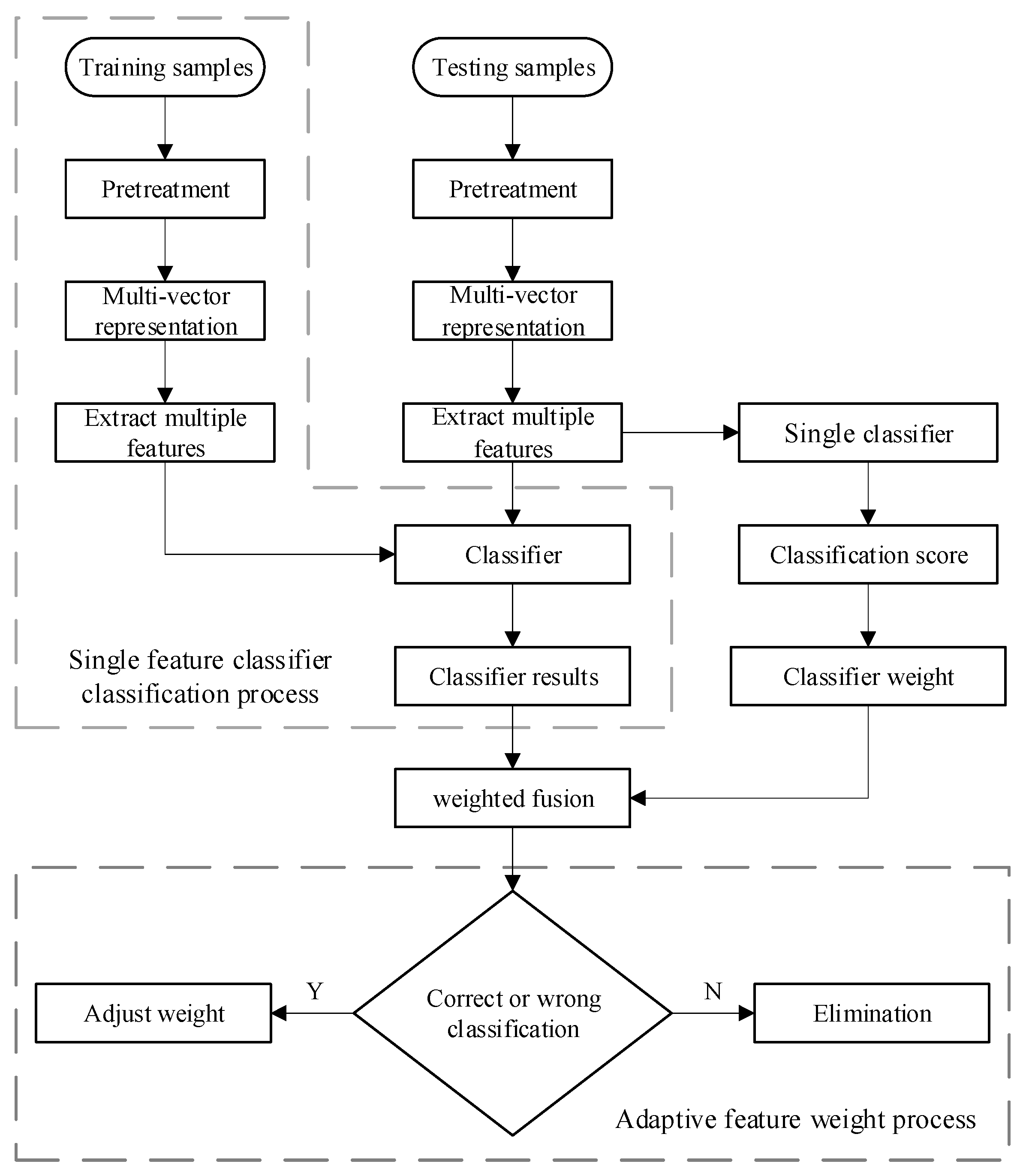
2.2. The Weighted Fusion Classification Algorithm
- (1)
- Suppose there are m classes of training samples. represents the set of training samples from the i-th class. represents the image vector representation of the j-th training sample of the c class and n is the number of training samples of the i-th class. The multi-vector representation method proposed in Section 2.2 is used to extract the feature of the whole training sample and obtain the characteristic matrix D of multiple sets of training samples.where d is the feature dimensions and k is the k-th class feature. is the feature vector of the i-th training sample of the k-th class sample.
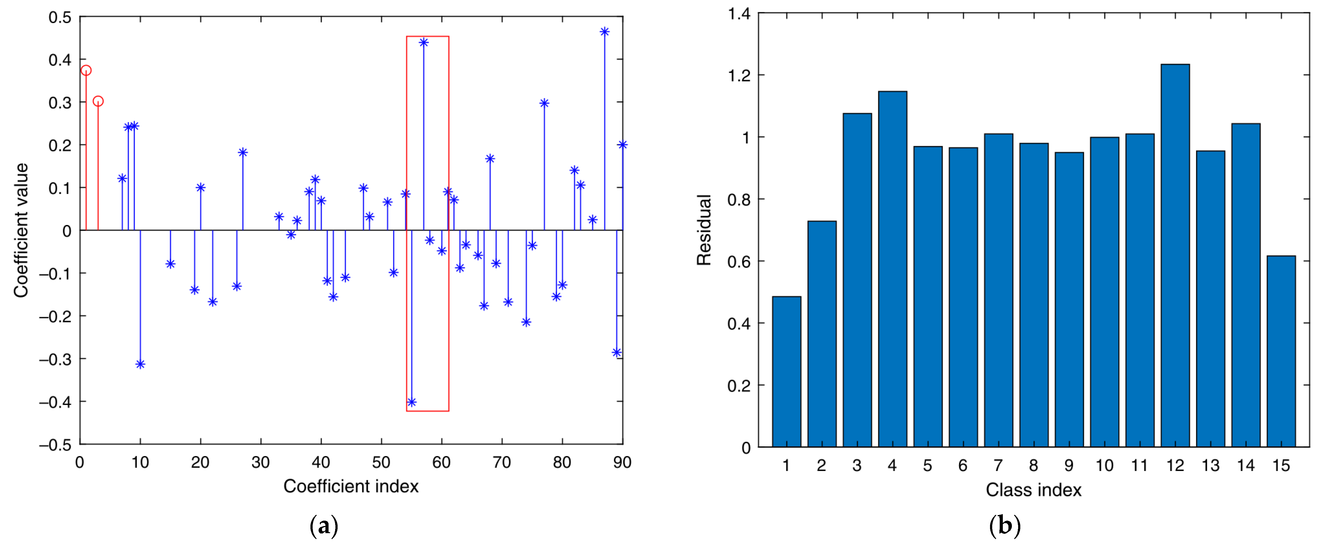
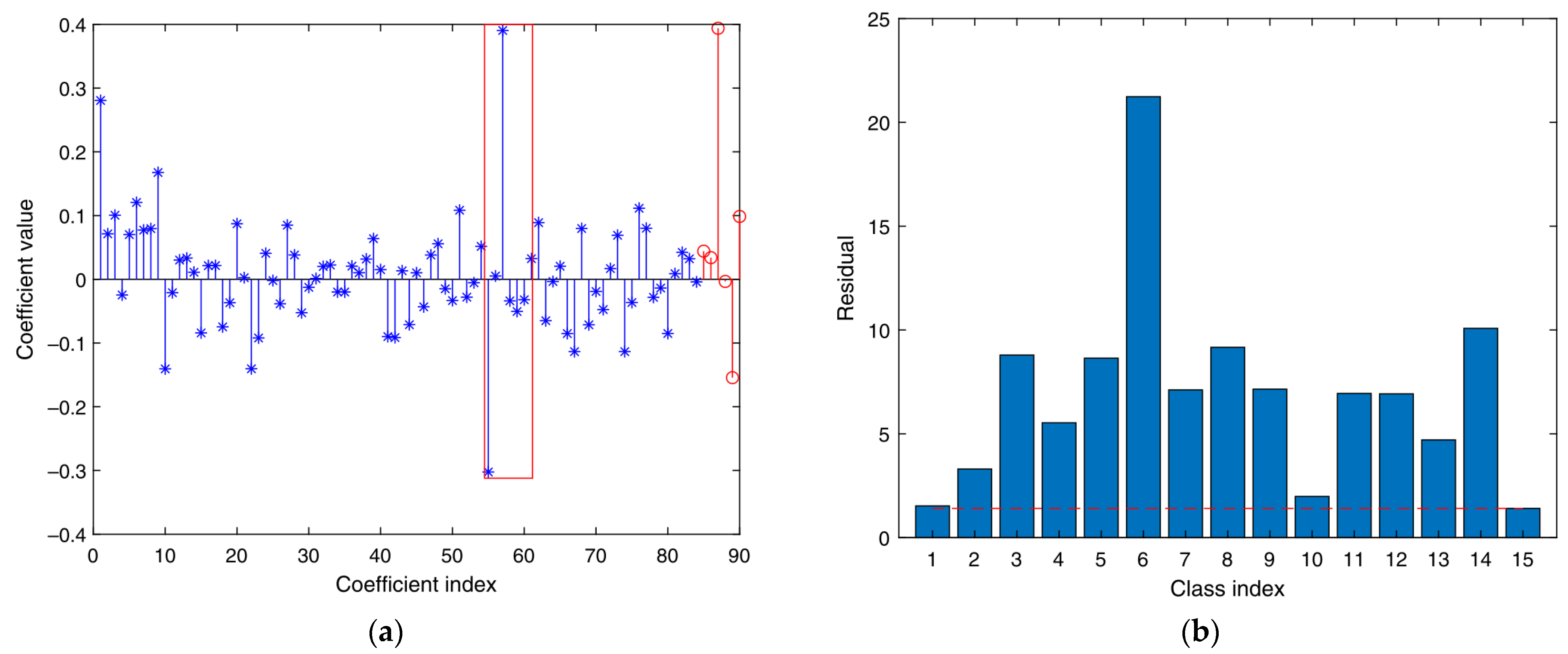
- (2)
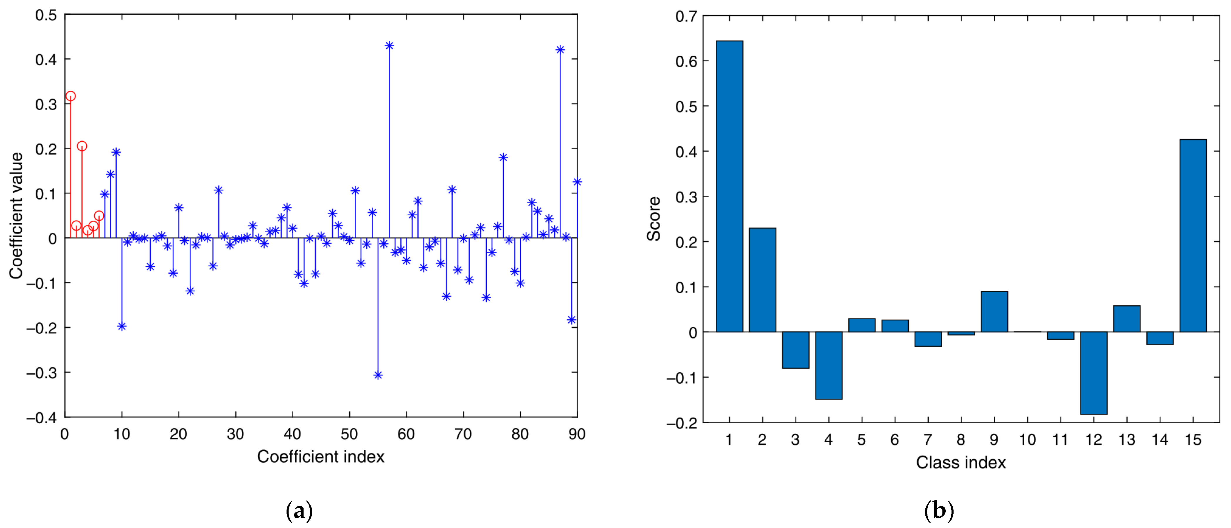
- Based on the methods in [21], corresponding sparse representation classifiers are generated for multiple feature vector matrices in (6). Multiple classifiers obtain the corresponding classification results of various sparse representations. Therefore, its residual is calculated via , where , . The degree of separation between different categories of the sparse classifier is obtained as follows:represents the degree of separation between the i-th sample of the k-th class classifier and the other classes in the whole training sample. The greater the separation degree, the more obvious the classification effect of the classifier on the training sample.
- (3)
- This study constructs and assigns initial weights for each sparse representation classifier. Using the degree of separation S of the first classifier output as the initial feature weight coefficient:represents the initialization weight ratio assigned to the i-th class sparse representation classification.
- (4)
- According to the weight coefficient of (8), the classification results are fused to determine the image category.. is the influence proportion of the j-th classifier to all samples under the influence of multi-classification fusion decision. We combine the classification result and its proportion value for linear weighting, and obtain the final classification result as follows:
- (5)
- This study iterates and optimizes the . of each classifier based on the validation data of the test samples, and use factor to adjust the weight ratio of each classifier. If all classifiers fail to detect rightly the vector representation of the sample is discarded. In the classification based on sparse representation, the weight coefficients are meaningful because they reflect the importance of each training sample.
3. The Analysis of the Proposed Algorithm
4. Experiments and Results
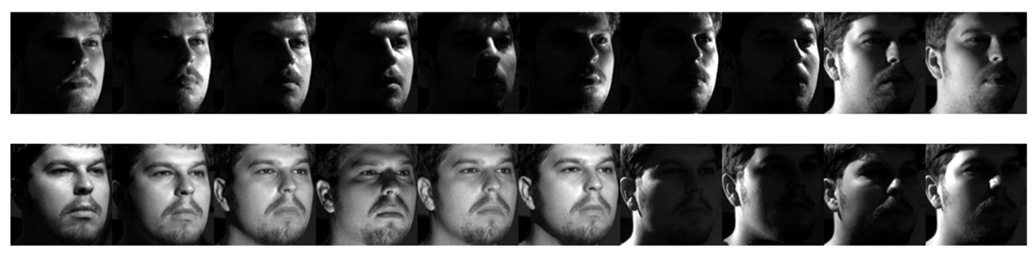
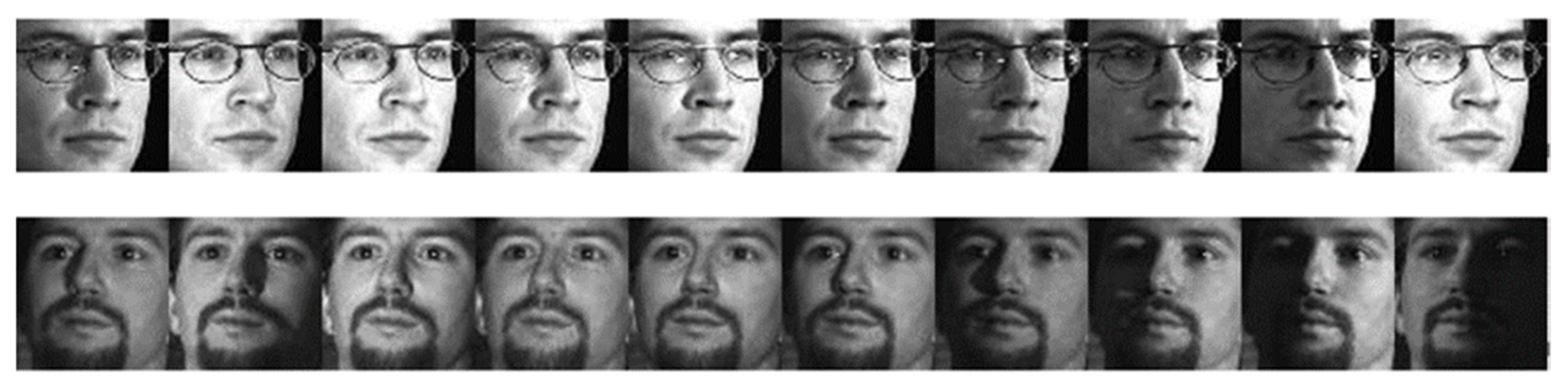
4.1. Experiments on the Extended Yale B Face Database
4.2. Experiments on the PIE Face Database
4.3. Experiments on the AR Face Database
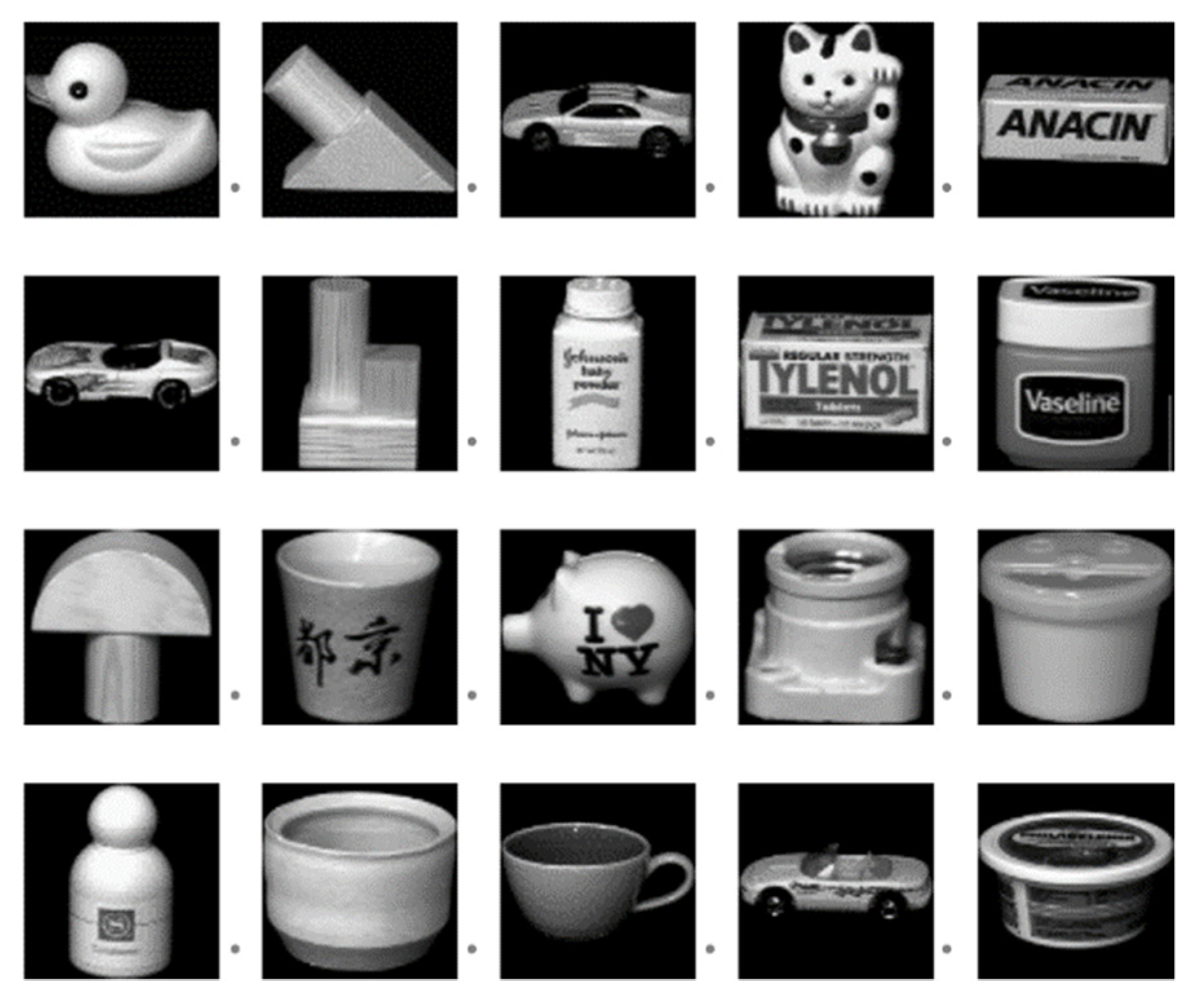
4.4. Experiments on the COIL-20 Database
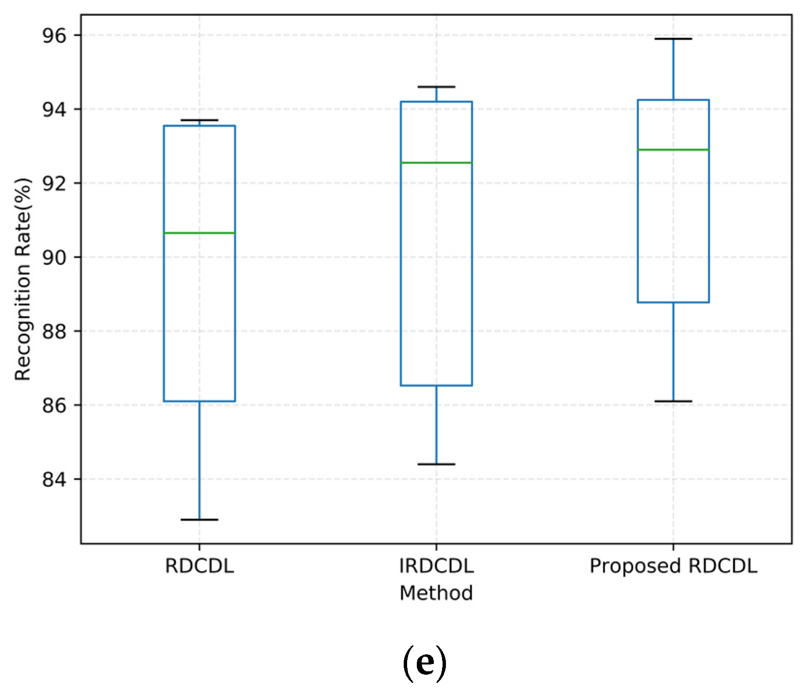
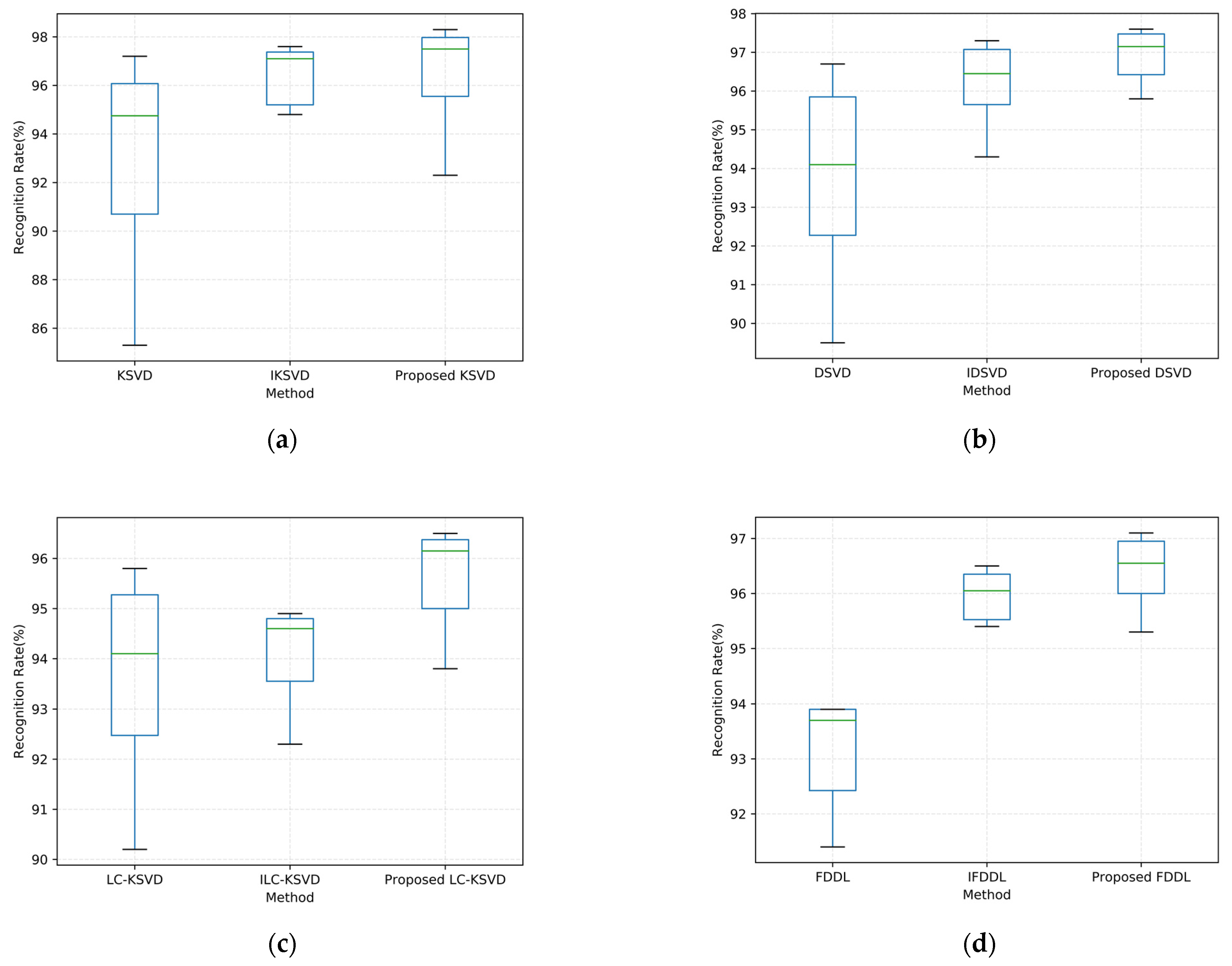
4.5. Statistical Tests
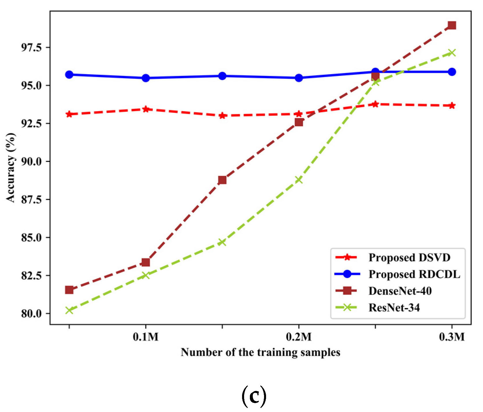
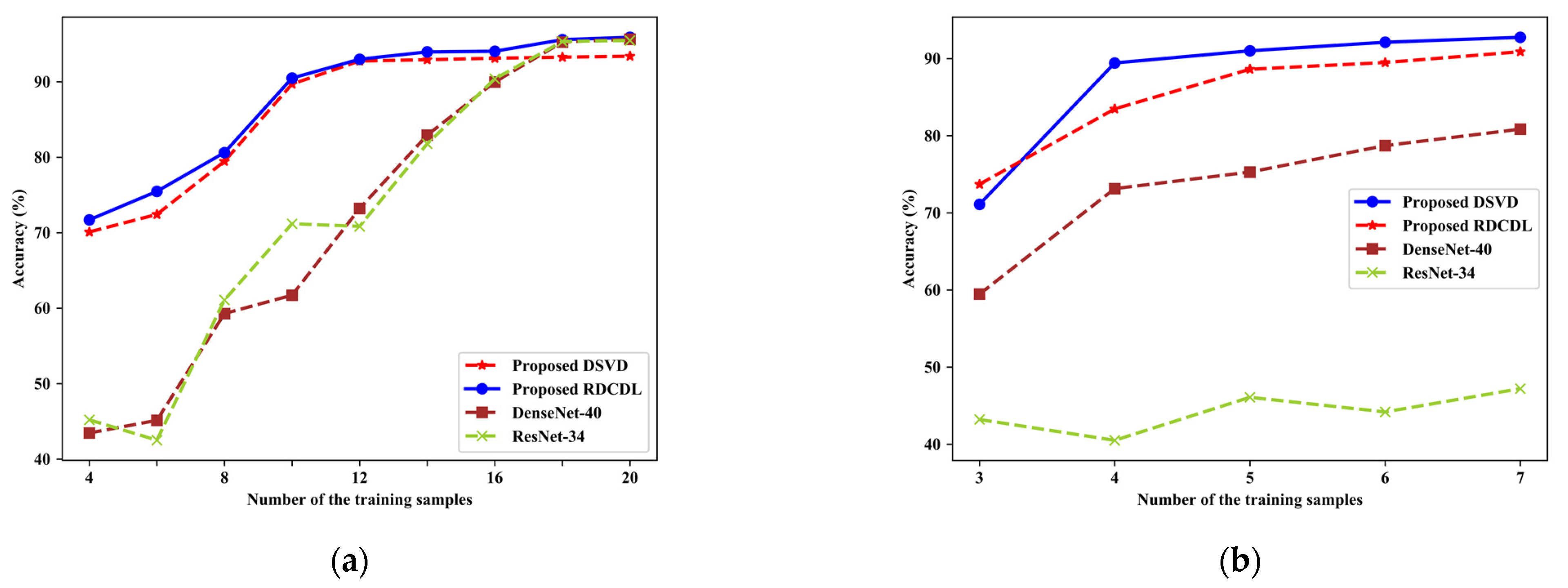
4.6. Comparison with Deep Learning Methods
5. Conclusions
Author Contributions
Funding
Data Availability Statement
Conflicts of Interest
References
- Zhang, J.; Liu, W.; Bo, L.; Zhang, H.; Li, H.; Xu, S. Joint Reflectance Field Estimation and Sparse Representation for Face Image Illumination Preprocessing and Recognition. Neural Process. Lett. 2020, 1–14. [Google Scholar] [CrossRef]
- Wang, L.; Li, T. Research on Image Feature Extraction Method Fusing HOG and Canny Algorithm. In Proceedings of the 2021 4th International Conference on Data Science and Information Technology, Shanghai, China, 23–25 July 2021; pp. 208–211. [Google Scholar]
- Lacombe, T.; Favreliere, H.; Pillet, M. Modal features for image texture classification. Pattern Recognit. Lett. 2020, 135, 249–255. [Google Scholar] [CrossRef]
- Li, Y.; Liu, J.; Tang, Z.; Lei, B. Deep spatial-temporal feature fusion from adaptive dynamic functional connectivity for MCI identification. IEEE Trans. Med. Imaging 2020, 39, 2818–2830. [Google Scholar] [CrossRef] [PubMed]
- Zhu, X.; Li, X.; Zhang, S. Block-row sparse multiview multilabel learning for image classification. IEEE Trans. Cybern. 2015, 46, 450–461. [Google Scholar] [CrossRef]
- Luo, Y.; Liu, T.; Tao, D.; Xu, C. Multiview matrix completion for multilabel image classification. IEEE Trans. Image Process. 2015, 24, 2355–2368. [Google Scholar] [CrossRef] [Green Version]
- Aharon, M.; Elad, M.; Bruckstein, A. K-SVD: An algorithm for designing overcomplete dictionaries for sparse representation. IEEE Trans. Signal Process. 2006, 54, 4311–4322. [Google Scholar] [CrossRef]
- Xu, Y.; Zhong, Z.; Yang, J.; You, J.; Zhang, D. A new discriminative sparse representation method for robust face recognition via l2 regularization. IEEE Trans. Neural Netw. Learn. Syst. 2016, 28, 2233–2242. [Google Scholar] [CrossRef]
- Li, Z.; Lai, Z.; Xu, Y.; Yang, J.; Zhang, D. A locality-constrained and label embedding dictionary learning algorithm for image classification. IEEE Trans. Neural Netw. Learn. Syst. 2015, 28, 278–293. [Google Scholar] [CrossRef]
- Zhang, H.; Wang, F.; Chen, Y.; Zhang, W.; Wang, K.; Liu, J. Sample pair based sparse representation classification for face recognition. Expert Syst. Appl. 2016, 45, 352–358. [Google Scholar] [CrossRef]
- Xian, Y.; Akata, Z.; Sharma, G.; Nguyen, Q.; Hein, M.; Schiele, B. Latent embeddings for zero-shot classification. In Proceedings of the IEEE Conference on Computer Vision and Pattern Recognition, Las Vegas, NV, USA, 27–30 June 2016; pp. 69–77. [Google Scholar]
- Gao, J.; Xu, L. A novel spatial analysis method for remote sensing image classification. Neural Process. Lett. 2016, 43, 805–821. [Google Scholar] [CrossRef]
- Albukhanajer, W.A.; Jin, Y.; Briffa, J.A. Classifier ensembles for image identification using multi-objective Pareto features. Neurocomputing 2017, 238, 316–327. [Google Scholar] [CrossRef]
- Zhang, Q.; Li, B. Discriminative K-SVD for dictionary learning in face recognition. In Proceedings of the 2010 IEEE Computer society Conference on Computer Vision and Pattern Recognition, San Francisco, CA, USA, 13–18 June 2010; pp. 2691–2698. [Google Scholar]
- Jiang, Z.; Lin, Z.; Davis, L.S. Label consistent K-SVD: Learning a discriminative dictionary for recognition. IEEE Trans. Pattern Anal. Mach. Intell. 2013, 35, 2651–2664. [Google Scholar] [CrossRef] [PubMed]
- Yang, M.; Zhang, L.; Feng, X.; Zhang, D. Fisher discrimination dictionary learning for sparse representation. In Proceedings of the 2011 International Conference on Computer Vision, Barcelona, Spain, 6–13 November 2011; pp. 543–550. [Google Scholar]
- Bacanin, N.; Stoean, R.; Zivkovic, M.; Petrovic, A.; Rashid, T.A.; Bezdan, T. Performance of a novel chaotic firefly algorithm with enhanced exploration for tackling global optimization problems: Application for dropout regularization. Mathematics 2021, 9, 2705. [Google Scholar] [CrossRef]
- Malakar, S.; Ghosh, M.; Bhowmik, S.; Sarkar, R.; Nasipuri, M. A GA based hierarchical feature selection approach for handwritten word recognition. Neural Comput. Appl. 2020, 32, 2533–2552. [Google Scholar] [CrossRef]
- Hu, C.; Wu, X.J.; Shu, Z.Q. Discriminative feature learning via sparse autoencoders with label consistency constraints. Neural Process. Lett. 2019, 50, 1079–1091. [Google Scholar] [CrossRef]
- Huang, Y.; Quan, Y.; Liu, T.; Xu, Y. Exploiting label consistency in structured sparse representation for classification. Neural Comput. Appl. 2019, 31, 6509–6520. [Google Scholar] [CrossRef]
- Xu, Y.; Li, Z.; Tian, C.; Yang, J. Multiple vector representations of images and robust dictionary learning. Pattern Recognit. Lett. 2019, 128, 131–136. [Google Scholar] [CrossRef]
- Liu, Z.; Wu, X.J.; Shu, Z. Multi-resolution dictionary collaborative representation for face recognition. Pattern Anal. Appl. 2021, 24, 1793–1803. [Google Scholar] [CrossRef]
- Zheng, S.; Zhang, Y.; Liu, W.; Zou, Y.; Zhang, X. A dictionary learning algorithm based on dictionary reconstruction and its application in face recognition. Math. Probl. Eng. 2020, 2020, 8964321. [Google Scholar] [CrossRef]
- Liu, Z.; Wu, X.J.; Yin, H.; Xu, T.; Shu, Z. Locality-Constrained Collaborative Representation with Multi-resolution Dictionary for Face Recognition. In Proceedings of the Chinese Conference on Pattern Recognition and Computer Vision (PRCV), Beijing, China, 29 October–1 November 2021; Springer: Berlin/Heidelberg, Germany, 2021; pp. 55–66. [Google Scholar]
- Fan, J.; Yang, C.; Udell, M. Robust Non-Linear Matrix Factorization for Dictionary Learning, Denoising, and Clustering. IEEE Trans. Signal Process. 2021, 69, 1755–1770. [Google Scholar] [CrossRef]
- Xu, Y.; Zhang, B.; Zhong, Z. Multiple representations and sparse representation for image classification. Pattern Recognit. Lett. 2015, 68, 9–14. [Google Scholar] [CrossRef]
- Lin, G.; Yang, M.; Yang, J.; Shen, L.; Xie, W. Robust, discriminative and comprehensive dictionary learning for face recognition. Pattern Recognit. 2018, 81, 341–356. [Google Scholar] [CrossRef]
- Li, L.; Peng, Y.; Qiu, G.; Sun, Z.; Liu, S. A survey of virtual sample generation technology for face recognition. Artif. Intell. Rev. 2018, 50, 1–20. [Google Scholar] [CrossRef]
- Li, H.; He, X.; Tao, D.; Tang, Y.; Wang, R. Joint medical image fusion, denoising and enhancement via discriminative low-rank sparse dictionaries learning. Pattern Recognit. 2018, 79, 130–146. [Google Scholar] [CrossRef]
- Zhang, Y.; Wang, Q.; Xiao, L.; Cui, Z. An improved two-step face recognition algorithm based on sparse representation. IEEE Access 2019, 7, 131830–131838. [Google Scholar] [CrossRef]
- Georghiades, A.S.; Belhumeur, P.N. Illumination cone models for faces recognition under variable lighting. In Proceedings of the CVPR98, Santa Barbara, CA, USA, 23–25 June 1998. [Google Scholar]
- Sim, T.; Baker, S.; Bsat, M. The CMU pose, illumination, and expression (PIE) database. In Proceedings of the Fifth IEEE International Conference on Automatic Face Gesture Recognition, Washington, DC, USA, 21–21 May 2002; pp. 53–58. [Google Scholar]
- Martinez, A.; Benavente, R. The AR Face Database: CVC Technical Report, 24; Autonomous University of Barcelona: Barcelona, Spain, 1998. [Google Scholar]
- Geusebroek, J.M.; Burghouts, G.J.; Smeulders, A.W. The Amsterdam library of object images. Int. J. Comput. Vis. 2005, 61, 103–112. [Google Scholar] [CrossRef]
- Iman, R.L.; Davenport, J.M. Approximations of the critical region of the fbietkan statistic. Commun. Stat. Theory Methods 1980, 9, 571–595. [Google Scholar] [CrossRef]
- Derrac, J.; García, S.; Molina, D.; Herrera, F. A practical tutorial on the use of nonparametric statistical tests as a methodology for comparing evolutionary and swarm intelligence algorithms. Swarm Evol. Comput. 2011, 1, 3–18. [Google Scholar] [CrossRef]
- He, K.; Zhang, X.; Ren, S.; Sun, J. Identity mappings in deep residual networks. In Proceedings of the European Conference on Computer Vision, Amsterdam, The Netherlands, 8–16 October 2016; Springer: Berlin/Heidelberg, Germany, 2016; pp. 630–645. [Google Scholar]
- Huang, G.; Liu, Z.; Van Der Maaten, L.; Weinberger, K.Q. Densely connected convolutional networks. In Proceedings of the IEEE Conference on Computer Vision and Pattern Recognition, Honolulu, HI, USA, 21–26 July 2017; pp. 4700–4708. [Google Scholar]
- Yi, D.; Lei, Z.; Liao, S.; Li, S.Z. Learning face representation from scratch. arXiv 2014, arXiv:1411.7923. [Google Scholar]


| The Number of Atoms | 38 | 76 | 114 | 152 | 190 | 228 | 266 | 304 | 342 | 380 |
|---|---|---|---|---|---|---|---|---|---|---|
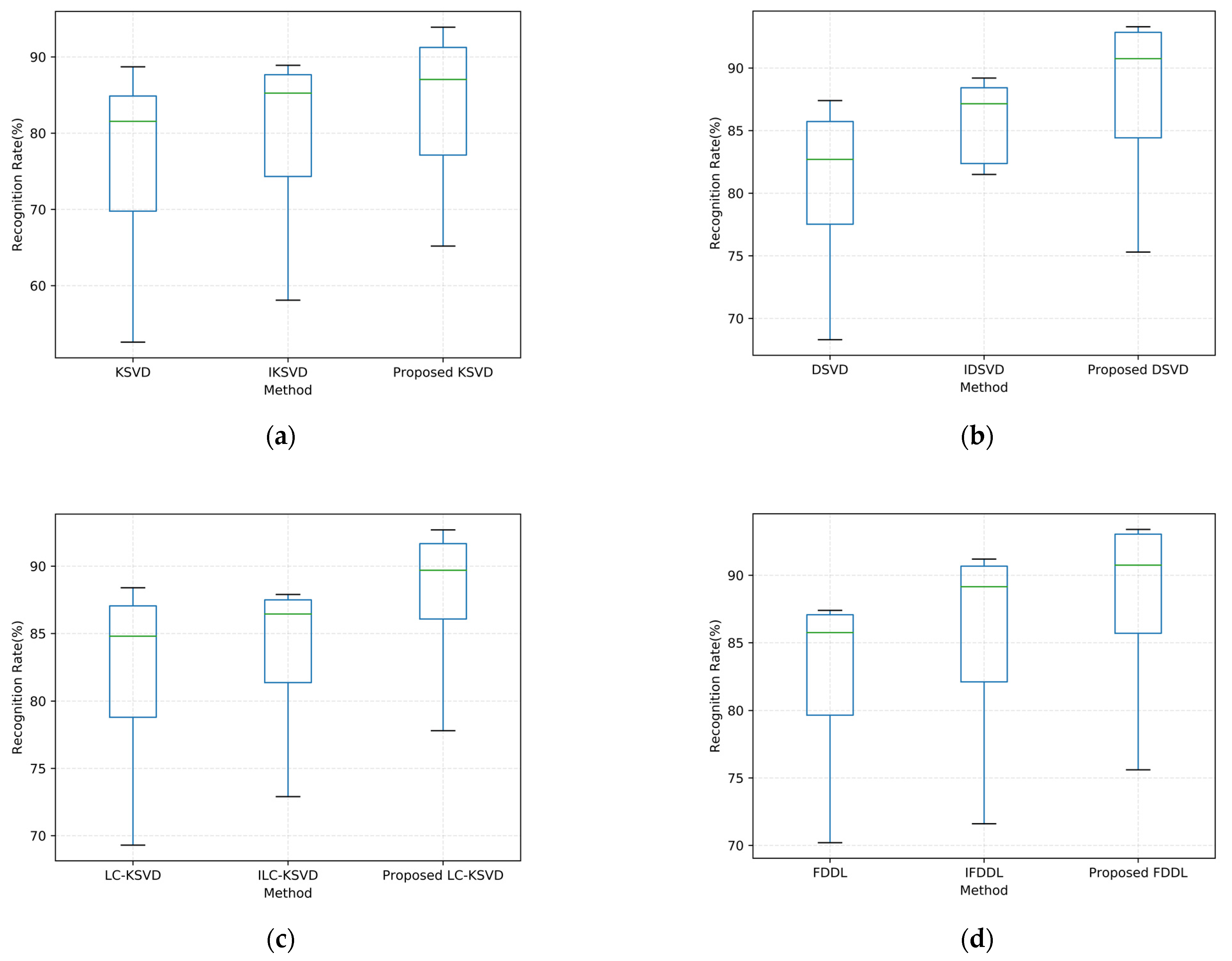
| KSVD | 55.2 | 68.0 | 75.1 | 80.2 | 82.9 | 85.3 | 86.2 | 83.6 | 52.6 | 88.7 |
| IKSVD | 58.1 | 72.4 | 80.1 | 84.0 | 86.5 | 87.9 | 88.3 | 87.0 | 63.8 | 88.9 |
| Proposed KSVD | 65.2 | 75.1 | 83.2 | 86.5 | 87.6 | 90.2 | 92.2 | 91.6 | 66.6 | 93.9 |
| DSVD | 52.4 | 68.3 | 76.4 | 80.9 | 84.1 | 85.8 | 87.4 | 87.1 | 85.5 | 81.3 |
| IDSVD | 54.1 | 72.9 | 81.5 | 85.0 | 87.2 | 88.5 | 89.2 | 88.9 | 88.2 | 87.1 |
| Proposed DSVD | 60.2 | 75.3 | 83.5 | 87.2 | 90.3 | 91.2 | 92.9 | 93.3 | 93.2 | 92.7 |
| LC-KSVD | 55.3 | 69.3 | 77.9 | 81.5 | 84.0 | 85.6 | 86.6 | 87.9 | 88.4 | 87.2 |
| ILC-KSVD | 55.4 | 72.9 | 80.5 | 83.9 | 85.9 | 87.0 | 87.5 | 87.9 | 87.9 | 87.5 |
| Proposed LC-KSVD | 60.4 | 77.8 | 85.2 | 88.7 | 89.4 | 90 | 90.7 | 92 | 92.7 | 92.3 |
| FDDL | 45.7 | 70.2 | 78.5 | 83.1 | 85.2 | 86.3 | 87.0 | 87.1 | 87.4 | 87.4 |
| IFDDL | 50.0 | 71.6 | 80.9 | 85.7 | 88.4 | 89.9 | 90.6 | 91.1 | 91.2 | 90.7 |
| Proposed FDDL | 60.1 | 75.6 | 84.4 | 89.6 | 90.3 | 91.2 | 92.9 | 93.3 | 93.4 | 93.1 |
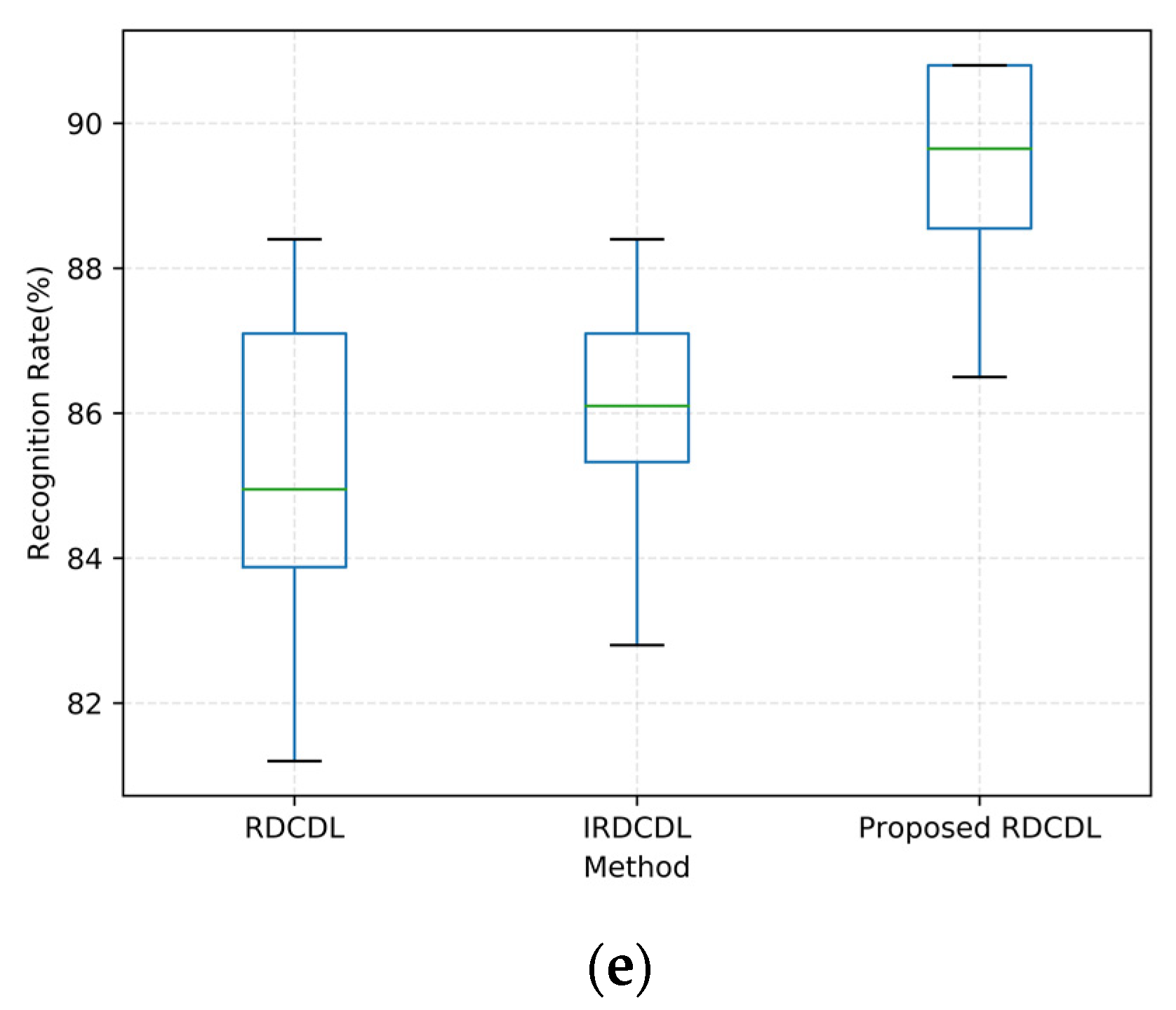
| RDCDL | 71.9 | 82.9 | 85.3 | 88.5 | 90.1 | 91.2 | 93.4 | 93.6 | 93.6 | 93.7 |
| IRDCDL | 73.6 | 84.4 | 85.4 | 89.9 | 91.9 | 93.2 | 93.9 | 94.3 | 94.6 | 94.6 |
| Proposed RDCDL | 76.2 | 86.1 | 88.2 | 90.5 | 92.6 | 93.2 | 93.2 | 94.6 | 95.6 | 95.9 |
| The Number of Atoms | 68 | 136 | 204 | 272 | 340 |
|---|---|---|---|---|---|
| KSVD | 63.7 | 68.1 | 71.4 | 74.9 | 77.2 |
| IKSVD | 68.4 | 75.4 | 78.6 | 81.2 | 82.4 |
| Proposed KSVD | 72.5 | 77.4 | 82.3 | 85.4 | 88.1 |
| DSVD | 63.8 | 68.3 | 73.1 | 75.3 | 77.7 |
| IDSVD | 69.2 | 77.7 | 81.1 | 82.5 | 83.4 |
| Proposed DSVD | 73.4 | 83.2 | 85.1 | 88.7 | 89.4 |
| LC-KSVD | 62.8 | 73.0 | 72.6 | 74.3 | 76.4 |
| ILC-KSVD | 67.9 | 79.3 | 77.7 | 76.5 | 75.5 |
| Proposed LC-KSVD | 72.2 | 83.4 | 84.7 | 83.1 | 83.4 |
| FDDL | 47.6 | 69.9 | 75.5 | 78.5 | 80.1 |
| IFDDL | 57.2 | 76.5 | 81.4 | 82.9 | 83.8 |
| Proposed FDDL | 68.4 | 80.4 | 84.5 | 86.7 | 87.4 |
| RDCDL | 75.7 | 81.1 | 83.4 | 82.9 | 84.2 |
| IRDCDL | 78.2 | 85.6 | 85.7 | 84.1 | 85.6 |
| Proposed RDCDL | 79.1 | 86.8 | 87.5 | 87.4 | 88.5 |
| The Number of Atoms | 120 | 240 | 360 | 480 | 600 | 720 | 840 | 960 | 1080 | 1200 |
|---|---|---|---|---|---|---|---|---|---|---|
| KSVD | 85.3 | 89.9 | 93.1 | 94.3 | 95.2 | 96.0 | 96.4 | 96.1 | 79.8 | 97.2 |
| IKSVD | 91.0 | 94.8 | 96.4 | 97.0 | 97.3 | 97.6 | 97.6 | 97.4 | 80.1 | 97.2 |
| Proposed KSVD | 92.3 | 95.1 | 96.9 | 97.4 | 97.9 | 98.0 | 98.1 | 98.3 | 94.5 | 97.6 |
| DSVD | 82.8 | 89.5 | 92.0 | 93.6 | 94.6 | 95.4 | 96.2 | 96.0 | 93.1 | 96.7 |
| IDSVD | 90.2 | 94.3 | 95.5 | 96.3 | 96.6 | 97.0 | 97.3 | 97.2 | 96.1 | 97.1 |
| Proposed DSVD | 91.0 | 95.8 | 96.4 | 97.0 | 97.5 | 97.6 | 97.6 | 97.4 | 96.5 | 97.3 |
| LC-KSVD | 86.8 | 90.2 | 92.7 | 93.7 | 94.5 | 94.9 | 95.4 | 95.4 | 95.8 | 92.4 |
| ILC-KSVD | 88.7 | 92.3 | 94.0 | 94.5 | 94.7 | 94.8 | 94.9 | 94.9 | 94.8 | 93.4 |
| Proposed LC-KSVD | 90.3 | 93.8 | 96.1 | 96.2 | 96.3 | 96.4 | 96.4 | 96.5 | 95.9 | 94.7 |
| FDDL | 83.4 | 91.4 | 92.2 | 93.1 | 93.5 | 93.9 | 93.9 | 93.9 | 93.9 | 93.9 |
| IFDDL | 86.6 | 94.1 | 95.4 | 95.9 | 96.0 | 96.2 | 96.4 | 96.4 | 96.5 | 96.1 |
| Proposed FDDL | 88.7 | 95.3 | 95.9 | 96.3 | 96.4 | 96.7 | 97 | 97 | 97.1 | 96.8 |
| RDCDL | 81.2 | 85.2 | 84.1 | 84.7 | 83.8 | 81.7 | 86.8 | 87.5 | 87.2 | 88.4 |
| IRDCDL | 82.8 | 86.1 | 85.7 | 85.2 | 86.1 | 82.6 | 86.5 | 87.5 | 87.3 | 88.4 |
| Proposed RDCDL | 84.2 | 86.5 | 88.5 | 88.7 | 89.1 | 90.2 | 90.8 | 90.8 | 90.8 | 90.8 |
| The Number of Atoms | 40 | 60 | 80 | 100 | 120 | 140 | 160 | 180 | 200 |
|---|---|---|---|---|---|---|---|---|---|
| KSVD | 82.5 | 85.5 | 87.2 | 88.0 | 88.4 | 89.0 | 89.5 | 84.7 | 89.0 |
| IKSVD | 84.0 | 86.8 | 88.2 | 89.1 | 89.3 | 89.5 | 89.8 | 90.3 | 89.0 |
| Proposed KSVD | 86.3 | 89.7 | 90.3 | 91.9 | 93.1 | 93.3 | 93.2 | 92.6 | 90.3 |
| DSVD | 84.3 | 85.6 | 86.9 | 87.5 | 88.5 | 89.1 | 88.7 | 87.0 | 84.1 |
| IDSVD | 84.6 | 86.8 | 88.0 | 89.0 | 89.6 | 90.0 | 90.0 | 89.9 | 89.0 |
| Proposed DSVD | 85.7 | 88.8 | 90.7 | 90.9 | 91.2 | 93.1 | 93 | 92.7 | 92.6 |
| LC-KSVD | 84.7 | 87.8 | 88.3 | 88.7 | 89.2 | 89.1 | 89.1 | 88.9 | 89.4 |
| ILC-KSVD | 85.3 | 88.9 | 89.7 | 90.2 | 90.5 | 90.6 | 90.5 | 90.8 | 90.5 |
| Proposed LC-KSVD | 86.3 | 89.9 | 90.4 | 92.3 | 93.2 | 93.3 | 93.4 | 93.4 | 93.2 |
| FDDL | 84.5 | 87.8 | 88.2 | 89.2 | 89.9 | 89.9 | 90.6 | 90.6 | 91.1 |
| IFDDL | 80.5 | 86.5 | 89.1 | 89.1 | 91.1 | 91.3 | 91.7 | 91.9 | 91.8 |
| Proposed FDDL | 84.0 | 86.9 | 91.2 | 91.2 | 92 | 92 | 92.2 | 92.3 | 92.5 |
| RDCDL | 84.8 | 87.5 | 89.4 | 88.5 | 90.2 | 91.4 | 92.1 | 92.1 | 92.9 |
| IRDCDL | 85.2 | 87.3 | 89.3 | 89.5 | 90.7 | 91.6 | 92.9 | 92.3 | 93.0 |
| Proposed RDCDL | 86.9 | 89.1 | 90.1 | 91.9 | 93.5 | 93.6 | 94.1 | 94.3 | 94.1 |
| Algorithms | Friedman |
|---|---|
| KSVD | 13.5 |
| IKSVD | 10.25 |
| Proposed KSVD | 4.5 |
| DSVD | 13 |
| IDSVD | 7.75 |
| Proposed DSVD | 3.25 |
| LC-KSVD | 11.25 |
| ILC-KSVD | 9.25 |
| Proposed LC-KSVD | 4.75 |
| FDDL | 12.25 |
| IFDDL | 8.25 |
| Proposed FDDL | 4.25 |
| RDCDL | 7.5 |
| IRDCDL | 6.25 |
| Proposed RDCDL | 4 |
| Statistic | 33.875 |
| 4.593 | |
| CD | 3.049 |
| p-value | 0.002150951 |
| Methods | Ext. Yale B | AR | CASIA-WebFace |
|---|---|---|---|
| Proposed DSVD | 93.39 | 92.76 | 93.44 |
| Proposed RDCDL | 95.90 | 90.89 | 95.37 |
| ResNet-34 | 95.47 | 47.21 | 97.15 |
| DenseNet-40 | 95.63 | 80.85 | 98.95 |
| Methods | Average Training Time | Average Testing Time |
|---|---|---|
| Proposed DSVD | 67.53 s | 0.85 s |
| Proposed RDCDL | 73.55 s | 0.87 s |
| ResNet-34 | 2.5 h | 2.16 s |
| DenseNet-40 | 3.2 h | 2.04 s |
Publisher’s Note: MDPI stays neutral with regard to jurisdictional claims in published maps and institutional affiliations. |
© 2022 by the authors. Licensee MDPI, Basel, Switzerland. This article is an open access article distributed under the terms and conditions of the Creative Commons Attribution (CC BY) license (https://creativecommons.org/licenses/by/4.0/).
Share and Cite
Pan, C.; Zhang, Y.; Wang, Z.; Cui, Z. Improved Multiple Vector Representations of Images and Robust Dictionary Learning. Electronics 2022, 11, 847. https://doi.org/10.3390/electronics11060847
Pan C, Zhang Y, Wang Z, Cui Z. Improved Multiple Vector Representations of Images and Robust Dictionary Learning. Electronics. 2022; 11(6):847. https://doi.org/10.3390/electronics11060847
Chicago/Turabian StylePan, Chengchang, Yongjun Zhang, Zewei Wang, and Zhongwei Cui. 2022. "Improved Multiple Vector Representations of Images and Robust Dictionary Learning" Electronics 11, no. 6: 847. https://doi.org/10.3390/electronics11060847
APA StylePan, C., Zhang, Y., Wang, Z., & Cui, Z. (2022). Improved Multiple Vector Representations of Images and Robust Dictionary Learning. Electronics, 11(6), 847. https://doi.org/10.3390/electronics11060847