Article

Hybridizing of Whale and Moth-Flame Optimization Algorithms to Solve Diverse Scales of Optimal Power Flow Problem

1
Faculty of Computer Engineering, Najafabad Branch, Islamic Azad University, Najafabad 8514143131, Iran
2
Big Data Research Center, Najafabad Branch, Islamic Azad University, Najafabad 8514143131, Iran
3
Centre for Artificial Intelligence Research and Optimisation, Torrens University Australia, Brisbane 4006, Australia
4
Yonsei Frontier Lab, Yonsei University, Seoul 03722, Korea
5
Departamento de Innovación Basada en la Información y el Conocimiento, Universidad de Guadalajara, CUCEI, Guadalajara 44430, Mexico
*
Authors to whom correspondence should be addressed.
Electronics 2022, 11(5), 831; https://doi.org/10.3390/electronics11050831
Submission received: 31 January 2022 / Revised: 26 February 2022 / Accepted: 1 March 2022 / Published: 7 March 2022

Abstract

:
The optimal power flow (OPF) is a practical problem in a power system with complex characteristics such as a large number of control parameters and also multi-modal and non-convex objective functions with inequality and nonlinear constraints. Thus, tackling the OPF problem is becoming a major priority for power engineers and researchers. Many metaheuristic algorithms with different search strategies have been developed to solve the OPF problem. Although, the majority of them suffer from stagnation, premature convergence, and local optima trapping during the optimization process, which results in producing low solution qualities, especially for real-world problems. This study is devoted to proposing an effective hybridizing of whale optimization algorithm (WOA) and a modified moth-flame optimization algorithm (MFO) named WMFO to solve the OPF problem. In the proposed WMFO, the WOA and the modified MFO cooperate to effectively discover the promising areas and provide high-quality solutions. A randomized boundary handling is used to return the solutions that have violated the permissible boundaries of search space. Moreover, a greedy selection operator is defined to assess the acceptance criteria of new solutions. Ultimately, the performance of the WMFO is scrutinized on single and multi-objective cases of different OPF problems including standard IEEE 14-bus, IEEE 30-bus, IEEE 39-bus, IEEE 57-bus, and IEEE118-bus test systems. The obtained results corroborate that the proposed algorithm outperforms the contender algorithms for solving the OPF problem.

Graphical Abstract

1. Introduction

The most fundamental component of a power system is the ability to provide power demand at the lowest possible operational cost while adhering to various technological, economic, and certain system constraints [1]. The optimal power flow (OPF) plays a vital role as an important tool to discover the optimal decision variables of a power network to minimize intended objectives. Since the introduction of the OPF problem by Carpintier in 1962 [2], many researchers proposed various approaches including quadratic programming [3], nonlinear programming [4], interior point [5], and Newton algorithm [6,7] to solve this nonlinear and non-convex problem. However, these traditional approaches cannot provide competitive results in the case of multi-objective nonlinear functions as they mostly sink into the local optimum. Hence, designing optimizers with effective search strategies which can deal with such complexities and provide competitive results is still an open issue for solving the OPF problem.
Metaheuristic algorithms are a subset of stochastic algorithms that have been employed for solving complex problems such as feature selection [8,9,10,11,12], engineering [13,14,15,16,17,18,19,20,21,22,23,24,25,26], community detection [27,28,29,30], and continuous optimization [31,32,33,34,35,36,37] problems. Metaheuristic algorithms employ stochastic techniques to discover the promising areas by exploring the search space in early iterations and improve solutions quality by exploiting the promising areas in the final iterations. The main categorization of the metaheuristic algorithms is depending on the source of inspiration which divides them into the evolutionary and the swarm intelligence (SI) algorithms [38]. The evolutionary algorithms mostly mimic natural biological evolution and reproduction to improve the randomly generated solutions. Genetic algorithm (GA) [39], differential evolution (DE) [40], and evolution strategies (ES) [41] are prominent optimizers inspired by evolutionary concepts. As the evolutionary approach has proven to be a promising procedure, many researchers proposed improved versions of GA and DE algorithms for solving various problems [42,43,44,45].
The collective and cooperative behavior of biological organisms including fishes, birds, terrestrial animals, and insects is the basis of developing SI algorithms to solve optimization problems. The particle swarm optimization (PSO) [46] is a well-known SI algorithm that mimics the navigation behavior of bird flocks’ for generating solutions in optimization tasks. Dorigo et al. [47] simulated the collective behavior of some ants in nature by proposing the ant colony optimization (ACO) algorithm. The krill herd (KH) algorithm [48] is a successful simulation of the herding behavior of krill individuals which consists of three phases including krill random diffusion, foraging activity, and movement. The grey wolf optimizer (GWO) proposed by Mirjalili et al. [49] is also a SI algorithm based on the pack hierarchy approach to organizing the wolves based on their strength and responsibilities into four groups. The chimp optimization algorithm (ChOA) [50] mimics the social and sexual behavior of chimps to solve optimization problems. Starling murmuration optimizer (SMO) [51] is a recently proposed SI algorithm that models the stunning murmuration of starlings to solve the continuous and engineering optimization tasks. The SMO algorithm proposes a dynamic multi-flock and three search strategies including whirling, diving, and separating to provide the proper diversity throughout the population and strike a balance between search strategies.
The moth-flame optimization (MFO) [52] is a novel SI algorithm that simulates the spiral movement of moths around the light sources at night to perform optimization. Among numerous metaheuristic algorithms, the MFO stands out for its ease of use and low computational complexity. As a result, the MFO is used to solve a broad range of real-world problems, such as feature selection [53,54,55,56,57,58], and constraint engineering problems [59,60,61,62,63,64,65,66]. The MFO algorithm has an interesting concept of flames to preserve the best solutions, also it has an efficient global search strategy to explore the search space. However, the MFO suffers from weak exploitation and imbalance between search strategies which prevents it from converging toward the promising zone. Conversely, the whale optimization algorithm (WOA) [67] mathematically modeled the humpback whales’ hunting behavior using three search strategies. The search strategies proposed in WOA provide sufficient exploitation for different optimization tasks [68,69,70,71,72,73,74,75]. However, they cannot satisfy the needs of the exploration during the complex optimization tasks. Although many metaheuristic algorithms including MFO and WOA have been used to address the OPF problem, they are mostly not scalable or not suitable for handling multi-objective cases.
Therefore, this study is devoted to proposing an effective hybridizing of WOA with a modified MFO algorithm (WMFO) for solving the OPF problem. In this algorithm, first, a population partitioning mechanism is introduced to divide a population between search strategies. Then, the proposed WMFO algorithm is evolved using the WOA and modified MFO movement strategies. A greedy selection operator is considered as the acceptance criteria of the new positions by comparing their previous fitness and the new ones. Moreover, a randomized boundary handling method is used to return the solutions that have violated the permissible boundaries of search space. Moreover, to bypass the local optimum traps, a self-memory mechanism is defined for each search agent to preserve the best so far experience. Finally, the performance of the proposed WMFO algorithm is evaluated to solve diverse power system scale sizes including the standard IEEE 14-bus, IEEE 30-bus, IEEE 39-bus, IEEE 57-bus, and IEEE 118-bus test systems. The simulation results are compared to seven prominent optimization algorithms including PSO [46], GWO [49], MFO [52], WOA [67], Levy-flight moth-flame optimization (LMFO) [76], chimp optimization algorithm (ChOA) [50], and moth-flame optimizer with sine cosine mechanisms (SMFO) [77]. According to the test results, WMFO outperforms other comparative algorithms in solving different power system scale sizes in both single and multi-objective cases of the OPD problem. The main contributions of this study are summarized as follows.
  • Proposing an effective hybridizing of WOA with a modified MFO to solve OPF problems with diverse power system scale sizes.
  • Proposing a population partitioning mechanism to divide a population between search strategies.
  • Introducing a modification of the canonical MFO using a self-memory mechanism to preserve the best so far experience.
  • Applying a randomized boundary handling method to return the solutions that have violated the permissible boundaries.
  • Applying a greedy selection operator to assess the acceptance criteria of new solutions.
  • The experiments’ results prove that the WMFO provides the best results in solving different scales of standard IEEE test systems compared to competitor algorithms.
The paper is organized as follows. A literature overview of the related works is included in Section 2. The formulation and objective functions of the OPF problem are presented in Section 3. The moth-flame and whale optimization algorithms are presented in Section 4. The proposed WMFO algorithm is comprehensively presented in Section 5. A rigorous evaluation of the effectiveness of the WMFO on the OPF problem is provided in Section 6. Statistical analysis is presented in Section 7. Ultimately, Section 8 summarizes the conclusions and suggests future works.

2. Related Works

The optimal power flow (OPF) problem is formulated as a complex nonlinear nonconvex constrained optimization problem with different objectives and a variety of IEEE bus test systems [78]. Many traditional methods, such as quadratic programming [79], linear and nonlinear programming [4,80], and Newton algorithm [6] have been applied to solve the OPF problem. Although, these methods are not suitable for solving practical systems due to the characteristics of nonlinear functions such as value-point effect and prohibited operating zones. Moreover, increasing the number of system buses intensifies the mentioned complexities and leads the algorithm toward sinking in local minimum solutions [81,82].
Recently, many metaheuristic optimization algorithms such as particle swarm optimization (PSO) [83], ant colony optimization (ACO) [84], shuffled frog leaping (SFL) [85], differential evolution (DE) [86], biogeography-based optimization (BBO) [87], gravitational search algorithm (GSA) [88], firefly algorithm (FA) [89], teaching-learning-based optimization (TLBO) [90], grey wolf optimizer (GWO) [91], ant lion optimizer (ALO) [92], moth-flame optimization (MFO) [93], crow search algorithm (CSA) [94], salp swarm algorithm (SSA) [95], Levy spiral flight equilibrium optimizer (LSFEO) [96], and jellyfish search optimizer (JS) [97], have been applied as significant problem solvers to cope with the weaknesses of the traditional algorithms in solving the OPF problem benchmarks. Moreover, many researchers applied metaheuristic algorithms to solve real power systems [98,99].
Sivasubramani et al. [100] proposed a multi-objective harmony search (MOHS) algorithm to solve the OPF problem. To identify the Pareto optimum front, the MOHS algorithm uses a rapid elitist non-dominated sorting and crowding distance. Then, a fuzzy-based mechanism is performed for selecting a compromise solution from the Pareto set. Improved particle swarm optimization (IPSO) [101] proposed a pseudo-gradient and the constriction factor to direct the particle’s velocity. The purpose of the pseudo-gradient is to identify the particle’s orientation so that they may swiftly converge to the best solution. Sinsuphan et al. [102] presented the improved harmony search method (IHS) by proposing a modification of the pitch adjustment rate to solve OPF problems with five standard IEEE test systems including 6-bus, 14-bus, 30-bus, 57-bus, and 118-bus. A hybrid algorithm based on a modified imperialistic competitive algorithm and teaching-learning algorithm named MICA–TLA [103] is proposed for solving the OPF problem. The results of the simulation were tested on the IEEE 30-bus and IEEE 57-bus test systems with various objective functions. In another study, Ghasemi et al. [78] introduced three modified techniques of the imperialistic competitive algorithm (ICA) based on three new actions that may occur to any colony for solving the OPF problem. The introduced techniques were justified in different cases of the IEEE 57- bus test system. Radosavljevic et al. [104] proposed a hybridization of particle swarm optimization and gravitational search algorithms (PSOGSA) to find a proper solution in power systems. The PSOGSA takes advantage of the social thinking of the PSO and the local search ability of the GSA.
An improved artificial bee colony (IABC) [105] optimizer is developed by orthogonal learning (OL) to empower the exploitation ability of the canonical ABC in solving the OPF problem. Fatima Daqaq et al. [106] brought up a multi-objective backtracking search algorithm (MOBSA) to solve the OPF problem. The MOBSA can solve the highly constrained objectives and find the best solution from all Pareto optimal solution set using a fuzzy membership technique integrated into the BSA algorithm. Li et al. [107] proposed a boosted adaptive differential evolution (JADE) with a self-adaptive penalty constraint management approach (EJADE-SP) to find the best solution to the OPF issue. The EJADE-SP algorithm used the crossover rate sorting mechanism to let individuals inherit more good genes, and re-randomizing parameters to sustain the population diversity and the effectiveness of the search. Furthermore, to speed up convergence, the EJADE-SP employs a dynamic population reduction method and a self-adaptive penalty constraint management technique to cope with various constraints. Nadimi et al. [108] brought up the improved grey wolf optimizer (I-GWO) using dimension learning-based hunting (DLH) search strategy. The DLH strategy maintains the diversity and equilibriums between local and global searches by constructing a neighborhood for each wolf. In [109], the slime mold algorithm (SMA) is used to solve the multi-objective OPF. The SMA mimics the oscillation mode of slime mold in nature and utilizes adaptive weights to mimic the process of providing positive and negative feedback in slime mold propagation waves.
Meng et al. [110] introduced a crisscross search-based grey wolf optimizer (CS-GWO) to solve IEEE test systems including 30-bus and 118-bus. The CS-GWO algorithm improved the hunting operation in GWO by incorporating a greedy operator and the horizontal crossover operator was then used to refine the positions of the top three wolves. Moreover, to preserve population variety and prevent premature convergence, the vertical crossover operator is used. Abd el-Sattar et al. [111] proposed an improved salp swarm algorithm (ISSA) for improving the movement strategies in canonical SSA to solve different OPF problems including 30, 57, and 118-bus test systems. ISSA utilizes a random mutation strategy to improve the exploration process and an adaptive process to enhance the exploitation process. In [112], a boosted whale optimization algorithm named EWOA-OPF is developed to boost the global search capability of the WOA in solving the OPF problem by employing Levy motion in the encircling phase and utilizing Brownian motion to work with a canonical bubble-net attack. Kahraman et al. [113] proposed an effective method by introducing a crowding distance-based Pareto archiving strategy to solve the multi-objective OPF problem. Akdag et al. [98] introduced the improved Archimedes optimization algorithm (IAOA) using the dimension learning-based strategy to build a neighborhood and spread the information flow between search agents.

3. Optimal Power Flow Problem

The optimal power flow (OPF) is considered a strategic instrument for designing and operating of power networks. The primary objective of OPF is to minimize a predefined objective function, such as the active power generation cost while satisfying the inequality and equality requirements of the system within the specified limitations. The OPF issue is shown mathematically in the following.

3.1. OPF Problem Formulation

The OPF is a non-convex and nonlinear problem that can be represented mathematically as follows:
M i n F ( x , u ) Subjected   to                g ( x , u ) = 0 ,         p = 1 ,   2 , ,     m h ( x , u ) 0 ,           p = 1 ,   2 , ,     j
where u is a vector that represents the independent (control) variables, F is the objective function to be optimized, x is the vector of dependent (state) variables, g and h are the equality and inequality constraints, m and j indicate the number of equality constraints and the number of inequality constraints, respectively. Moreover, the state variables of OPF represented in Equation (2) consist of slack bus power PG1, load bus voltage VL, transmission line loading Sl, and generator reactive power output QG,
x = [ P G 1 ,   V L 1 , , V L N L , Q G 1 , , Q G N G , S l 1 , , S l N T L ]
where NL indicates the number of load buses, NTL and NG are the number of transmission lines and generators, respectively. The control variables represented in Equation (3) are the independent variables including generator active power outputs PG (except at the slack bus PG1), generator voltages VG, transformer tap settings T, and shunt VAR compensations QC. NT indicates the number of the regulating transformer and NC denotes the number of VAR compensator units.
u = [ P G 2 ,   , P G N G , V G 1 , , V G N G , T 1 , , T N T , Q C 1 , , Q C N C ]

3.2. Constraints

The OPF problem has equality and inequality constraints that are handled during the optimization process. The representations of both constraints are expressed as follows.

3.2.1. Equality Constraints

The balance between active and reactive power flow is maintained by the equality constraints consisting of a set of nonlinear power flow formulations represented in Equations (4) and (5).
P G i P D i = | V i | j = 1 N B | V j | ( G i j c o s δ i j + B i j s i n δ i j )
Q G i Q D i = | V i | j = 1 N B | V j | ( G i j c o s δ i j + B i j s i n δ i j )
where NB denotes the number of buses, PGi and PDi are the generator active power and demand active power. QGi and QDi are the generator reactive power and demand reactive power. Bij and Gij represent susceptance and conductance. Moreover, δ i j represents the phase difference of voltages between bus i and bus j.

3.2.2. Inequality Constraints

The inequality constraints which are the operating limits for OPF problem limited by the lower and upper bounds are represented as follows:
  • Generator constraints
    P G i m i n P G i P G i m a x   ;       i = 1 , , N G
    Q G i m i n Q G i Q G i m a x   ;       i = 1 , , N G
    V G i m i n V G i V G i m a x   ;       i = 1 , , N G
  • Transformer tap setting constraints
    T m i n T i T m a x   ;         i = 1 , , N T
  • Shunt VAR compensator constraints
    Q c i m i n Q c i Q c i m a x   ;       i = 1 , , N C
  • Line power flow constraints
    S L i S L i m a x   ;                       i = 1 , , N T L

3.2.3. Inequality Constraints Handling

Although the control variables are constrained by themselves, the dependent variables’ inequality constraints including Sl, VL, PG1, and QG are appended to the objective function as a quadratic penalty term to maintain the dependent variables in their acceptable limits and to reject any impracticable solution. The expanded objective function may be represented mathematically as follows [114]:
P e n a l t y = λ P ( P G 1 P G 1 l i m ) 2 + λ V i = 1 N L ( V L i V L i l i m ) 2 + λ Q i = 1 N G ( Q G i Q G i l i m ) 2 + λ S i = 1 N T L ( S l i S l i l i m ) 2  
where λV, λP, λS, and λQ are the penalty factors. The initially specified factors are 106 for both load bus voltage (λV) and power generation output at the slack bus (λP), 103 for line loading (λS), and 104 for generator reactive power (λQ). In this paper, the limit of the variable x is denoted by the symbol xlim, which can be defined using Equation (13), where r is a random number in the intervals 0 and 1.
x l i m = { x m a x 0.25 × ( x m a x x m i n ) × r ,                   i f     x > x m a x x m i n 0.25 × ( x m a x x m i n ) × r ,                   i f     x < x m i n

3.3. OPF Objective Functions

In this work, two objectives are investigated to address the OPF problem: an economic problem, which refers to the reduction of overall fuel costs in power production, and a practical challenge of minimizing the voltage deviation.

3.3.1. Case 1: Minimization of Total Fuel Cost

Total fuel cost is formulated as a minimization problem with the single-objective function. The quadratic function approximates the relationship between fuel expense ($/h) and produced electricity (MW), based on Equation (14), where f1 refers to the total cost of generation ($/h). ai, bi, and ci are the cost coefficients of the i-th generator. All load buses are confined to 0.95 to 1.05 p.u. voltage range
f 1 = i = 1 N G ( a i + b i P G i + c i P G i 2 )

3.3.2. Case 2: Total Fuel Cost and Voltage Deviation Minimization

The goal of this objective function is to minimize both the cost of fuel and the voltage deviation simultaneously. This objective function’s mathematical expression is as follows:
f 2 = i = 1 N G ( a i + b i P G i + c i P G i 2 ) + W v i = 1 N L | V i 1 |
where Wv = 200 represents the weighting factor. To effectively address the multi-objective issue, Equation (15) is a single equation that incorporates two weighted objectives.

4. Preliminaries

This section presents the concepts and mathematical models of moth-flame optimization and whale optimization algorithm in detail.

4.1. Moth-Flame Optimization (MFO)

The MFO is a prominent algorithm that mimics the spiral motion of moths around light sources at night. This behavior comes from a navigation mechanism called transverse orientation which helps moths to fly a long distance in a straight path by preserving a constant angular relationship with the moon. For far light sources like the moon, the transverse orientation plays a navigation role for moths. However, when it comes to relatively closer artificial light sources, the transverse orientation causes the moths to follow a deadly spiral path around the light source. The MFO algorithm is a simulation of this behavior of moths facing artificial lights. Hence, moths and flames are two fundamental concepts used in the MFO algorithm. In this algorithm, the moths are the main search agents which can be represented by matrix M(t) as follows.
M ( t ) = [ m 11   m 1 d m 1 D m i 1 m i d m i D m N 1   m N d m N D ]
where mid is the value of d-dimension of i-th moth, N indicates the total number of moths that explore the D-dimensional search space in each iteration. Additionally, it is expected that there is a vector containing the corresponding fitness of each moth, as shown below.
O M ( t ) = [ O M 1 ( t ) O M 2 ( t ) O M N ( t ) ]
As mentioned earlier, flames are the second basic concept of the MFO algorithm, which leads the moths toward promising areas discovered in the previous iterations. Theoretically, the moths fly around their corresponding flames in a spiral path, which can be formulated in Equation (18),
M i ( t ) = D i ( t ) × e b k × C o s ( 2 π k ) + F j ( t )
D i ( t ) = | F c ( t ) M i ( t ) |
where Mi (t) represents the position of i-th moth in iteration t, the Di denotes the linear distance between Mi and its corresponding flame (Fc) which is formulated in Equation (19), b indicates the logarithmic helix shape constant defined spiral, k is a random value in [−1, 1], and Fj is the j-th flame’s position. Considering a unique flame for each moth ensures that the algorithm does not sink into the local optimum during the early iterations. Whereas the algorithm converges toward the promising zones by decreasing the number of flames using Equation (20), where t denotes the current iterations, N represents the total number of population and MaxIt determines the maximum number of iterations. Hence, in this algorithm j equals to FlamNum.
F l a m e N u m ( t ) = r o u n d ( N t × N 1 M a x I t   )

4.2. Whale Optimization Algorithm (WOA)

The humpback whales’ hunting behavior in nature is mathematically modeled in the WOA [67]. Humpback whales are mainly considered to be predators that surround and capture their prey using the bubble-net hunting strategy. In this algorithm, the best position discovered so far is designated as the prey position X* that guides other search agents toward a promising area during the exploitation phase. Encircling prey, spiral bubble-net attacking to enhance local search, and searching for prey to enhance global search are the three techniques of whales that are formulated in the WOA algorithm based on the following definitions [115].
Encircling prey: Humpback whales can detect and surround the position of prey. The WOA considers the current best whale X* is close to the target prey since it is impossible to determine the location of the global optimum solution a priori. In the next phase, the positions of other whales are changed toward the X* based on Equations (21) and (22),
D i s ( X * , X i ) = | C i ( t ) × X * ( t ) X i ( t ) |
X i ( t + 1 ) = X * ( t ) A i ( t ) × D i s ( X * , X i )
where, Dis (X*, Xi) specifies the distance between the prey and the i-th whale in the current iteration, A and C indicate coefficient values computed based on Equations (23) and (24).
A ( t ) = 2 × a ( t ) × r a ( t )
C i ( t ) = 2 × r
where a decreases from 2 to 0 throughout the iterations using Equation (25). Moreover, r generates a random value in the intervals 0 and 1.
a ( t ) = 2 t × ( 2 M a x I t )
Bubble-net attacking: A mathematical model of humpback whale bubble-net strategy (exploitation) has been developed using two methodologies named shrinking encircling mechanism and spiral updating position which are formulated in Equation (26),
X i ( t + 1 ) = { X * ( t ) A ( t ) × D i s ( X r , X i )                           i f   p < 0.5 D i s ( X * , X i ) × e b l × cos ( 2 π l ) + X * ( t )         i f   p 0.5
where p denotes a random value generated in [0, 1]. If the value of p is found to be smaller than 0.5, the position of Xi changes using a shrinking encircling mechanism. On the other hand, a spiral updating technique is used if the value of p is found to be greater than or equal to 0.5. A denotes a random variable generated in [−a, a], where a decreases from 2 to 0 throughout the iterations. Dis (X*, Xi) denotes the distance of i-th search agent and the prey in the spiral updating position, b denotes a constant value, and l denotes a random value in the range [−1, 1].
Searching for prey: To emphasize the exploration ability of the algorithm (when |A| ≥ 1), a whale’s location is updated using Equation (27), in which a random whale is chosen rather than the best whale discovered so far.
X i ( t + 1 ) = X r ( t ) A × D i s ( X r , X i )
where, Xr (t) represents the position of a randomly chosen whale in the current iteration and Dis (Xr, Xi) indicates the distance between i-th whale and Xr.

5. Proposed Algorithm

The ability to strike a balance between exploitation and exploration abilities is a crucial feature for any SI algorithm. As discussed earlier, the concept of the flame introduced in the MFO algorithm is regarded as an effective approach for maintaining the balance between exploration and exploitation by linearly decreasing the number of flames throughout the iterations. However, MFO inherently suffers from inefficient exploitation ability which results in stagnating in far from promising areas or premature convergence into local optima. On the other hand, the experimental results [116] reveal that the WOA benefits from efficient exploitation ability, while its exploration and the balance between search strategies are not sufficient to handle complex real-world problems, especially in the OPF problem. Therefore, this study is devoted to proposing a hybridization of whale and moth-flame optimization (WMFO) to effectively solve the OPF problem. The proposed WMFO introduces a population partitioning mechanism, movement strategies, randomized boundary handling, and a greedy selection operator.
Suppose the matrix X N D ( t ) = { X 1 ( t ) ,   , X i ( t ) , , X N ( t ) } as a finite set of positions in iteration t such that the vector X i ( t ) = [ x i 1 ,   , x i d , ,   x i D ] denotes the position of i-th individual in the D-dimensional search space. In the first iteration, the matrix X N D ( t ) is initiated using Equation (28),
x i d = r a n d d × ( U b d L b d ) + L b d
where x i d is the value of d-dimension, randd is a random number between intervals 0 and 1, and ubd and lbd are the upper bound and lower bound for d-dimension. For the rest of the iterations, the matrix X N D ( t )   is updated using movement search strategies in the proposed WMFO algorithm. Algorithm 1 presents the WMFO pseudo-code.
Algorithm 1. The pseudocode of the proposed WMFO algorithm
Input: Dimension size (D), Maximum iterations (MaxIt), and Number of search agents (N).
Output: The global best solution.
1.Begin
2. Initialize the population
3. Set the self-memory mechanism for each search agent using Definition 2.
4. Calculating the fitness values.
5. Set t = 1.
6.    While tMaxIt
7.          Constructing two subpopulations PopMFO and PopWOA using Definition 1.
8.          If t = = 1 then
9.              Constricting the matrix flames by ascending ordered the fitness values.
10.          Else
11.              Updating F(t) and OF(t) by the sorted search agents from matrices F(t) and X(t).
12.        End If
13.        For i = 1: N
14.            If iPopMFO then
15.                  Computing the FlameNum (t) using Equation (20).
16.                  If iFlameNum (t)
17.                        Computing Di based on Equation (19).
18.                        Updating the new position of Xi (t + 1) using Equations (18).
19.                  Else
20.                        Computing δi (t) based on Equation (31).
21.                        Updating the new position of Xi (t + 1) using Equations (30).
22.                  End If
23.            Else
24.                  If p < 0.5 then
25.                        If |A| ≥ 1 then
26.                                Updating the new position of Xi (t + 1) using Equation (27).
27.                        Else
28.                Updating the new position of Xi (t + 1) using Equation (22).
29.                        End If
30.                  Else
31.                        Updating the new position of Xi (t + 1) using Equation (26).
32.                  End If
33.            End If
34.            Checking and applying randomized boundary handling using Equation (32).
35.            Computing the fitness values, and updating Xbesti based on Definition 2.
36.          End for
37.          Applying the greedy selection operator using Equation (33).
38.          Updating the global best solution.
39.          t = t + 1.
40.        End while
Definition 1 (Population partitioning mechanism).
Given Pop = {PopMFO, PopWOA} is a finite set of two distinct subpopulations PopMFO and PopWOA with predefined capacity к. First, the members of the population are shuffled using a discrete uniform distribution and then divided between two matrices PopMFO and PopWOA such that PopMFO = {X1…Xк} and PopWOA = {Xк+1…XN}, where N represents the number of population. In this mechanism, each subpopulation evolves independently which causes the individuals to explore the search space from different perspectives. Hence, the flow of improper information is slowed down within the population and decreases the risk of premature convergence.
Movement strategies: The WMFO employs two movement strategies for evolving subpopulations PopWOA and PopMFO. The subpopulation PopWOA is updated using the WOA movement strategies while subpopulation PopMFO is updated based on the modified MFO movement strategy.
WOA movement strategies: The WMFO employs the canonical WOA’s movement strategies to update the positions of subpopulation PopWOA using Equation (29), where Xi (t + 1) represents the next position of i-th search agent and i P o p W O A .
x i ( t + 1 ) = { Encircling prey defined in Equation ( 12 )    p i < | | A | < 1 Search for prey defined in Equation ( 17 )    p i < | | A | 1 Bubble net attacking defined in Equation ( 16 )    p i 0.5
Modified MFO movement strategy: The proposed WMFO evolves the subpopulation PopMFO using Equation (30), where b is the constant value, k is a random value between intervals [−1, 1], and Fj denotes the j-th flame such that index j is computed using Equation (20). δ i ( t ) is computed using Equation (31), where Xbesti is the position of the self-memory mechanism defined using Definition 2.
X i ( t + 1 ) = δ i ( t ) × e b k × C o s ( 2 π k ) + F j ( t ) ,   where   i P o p M F O
δ i ( t ) = | F c ( t ) X i ( t ) | + ( 1 N i = 1 N X b e s t i ) X i ( t )
Definition 2 (Self-Memory mechanism).
Let SM = {SM1 … SMi … SMN} is a finite set of N search agents’ memories. The SMi is denoted by SMi = (Xbesti, Fbesti), where Xbesti represents the best position of Xi so far acquired, and Fbesti denotes the fitness of Xbesti. In the first iteration, Xbesti (t = 1) ← Xi (t = 1) and Fbesti (t = 1) ← OXi (t = 1). For the remaining iterations (t > 1), Xi and Fbesti are updated based on the best so far solution obtained by each Xi.
Randomized boundary handling: The canonical MFO and WOA use a simple mechanism for boundary limiting which assigns a value equal to its corresponding lower bound (lbd) if the d-th dimension of a search agent is less than the value of lbd. Conversely, a value equal to the corresponding upper bound (ubd) is given to the d-th dimension of a search agent if it is found to be greater than ubd. Although this boundary limiting method works efficiently for linear and convex problems, it leads the algorithm toward stagnation in the case of multi-objective nonlinear functions such as the OPF problem. Hence, to avoid stagnation, a randomized-based variable boundary limiting is introduced in the proposed WMFO based on Equation (32), where xid denotes the value of d-th dimension of i-th search agent, and r is a random value between intervals 0 and 1.
x i d ( t ) = { l b d + 0.25 × ( u b d l b d ) × r ,     i f   x i d ( t ) < l b d u b d 0.25 × ( u b d l b d ) × r ,     i f   x i d ( t ) > u b d
Greedy selection operator: WMFO employs the selection operator to evaluate the acceptance criteria of new solutions by comparing the fitness of new solutions OX(t + 1) with the fitness of previous population OX(t) using Equation (33).
X i ( t + 1 ) = { X i ( t + 1 )                             O X i ( t + 1 ) < O X i ( t ) X i ( t )                                   O X i ( t + 1 ) O X i ( t )

6. Experimental Evaluation

In this section, first, a sensitivity analysis is conducted on the modified MFO, WOA, and the proposed WMFO to investigate the exploration and exploitation abilities. Then, the numerical efficiency of the proposed WMFO is scrutinized using simulation studies carried out on two scenarios based on five IEEE bus test systems consisting of IEEE 14-bus, IEEE 30-bus, IEEE 39-bus, IEEE 57-bus, and IEEE 118-bus test systems, where MATPOWER [117] is used for load flow calculation. The acquired results are then compared with five well-known metaheuristic algorithms including particle swarm optimization (PSO) [46], grey wolf optimizer (GWO) [49], moth-flame optimization (MFO) [52], whale optimization algorithm (WOA) [67], chimp optimization algorithm (ChOA) [50], and two enhanced variants of MFO, Levy-flight moth-flame optimization (LMFO) [76], and synthesis of MFO with sine cosine mechanisms (SMFO) [77]. The parameters of the competitor algorithms were set the same as the recommended settings in their works, which are reported in Table 1.
The proposed WMFO and other comparative algorithms were run 20 times separately on Intel Core i7 (2.60 GHz) and 24 GB of RAM using MATLAB R2020 to ensure that all comparisons are fair. The maximum number of iterations (MaxIt) and population size were set to (D × 104)/N for the sensitivity analysis tests, where D and N are dimensions of the problem and 100, respectively. For the IEEE bus test systems, the MaxIt and N are set to 200 and 50, respectively. The best values of control variables (DVs) and objective variables are tabulated in Table 2, Table 3, Table 4, Table 5, Table 6, Table 7, Table 8, Table 9, Table 10 and Table 11, Table A1 and Table A2.

6.1. Impact Analysis of Hybridizing WOA and Modified MFO

The exploration and exploitation abilities of the WOA, modified MFO, WMFO are investigated on several test functions selected from the CEC 2018 benchmark suite [118]. The first function F1 is a unimodal function, which can be employed to assess the exploitation ability of the algorithms. The test function F9 is a multimodal function with many local optima, that is employed to investigate the exploration ability. Test functions 12, 14, and 19 are hybrid and 22, 25, 28, and 30 are composition functions that are suitable for evaluating the algorithms’ ability to prevent local optima and to strike balance between exploration and exploitation. The plotted convergence of these functions is presented in Figure 1.
Analyzing convergence behavior of the test function F1 shows that the convergence trend of the modified MFO is hampered by local optimum after the initial iterations, while the WOA maintained its descent slope till the half of iterations, which shows its better exploitation ability compared to the modified MFO. On the contrary, the proposed WMFO converges toward the global solution by effectively exploiting the search space in the early iterations. The test function F9 shows that the modified MFO has better exploration than the WOA, and the proposed hybridization of WOA and modified MFO achieves superior results by effectively exploring the search space. The convergence behavior of hybrid and composition functions reveals that although WOA and modified MFO cannot maintain the balance between their search strategies, the proposed hybridization of them maintains the balance between exploitation and exploration and bypasses the local optimum effectively.

6.2. IEEE Bus Test Systems

The IEEE 14-bus, IEEE 30-bus, IEEE 39-bus, IEEE 57-bus, and the IEEE 118-bus test systems are employed to test the simulation effect of the WMFO for solving the OPF problem in two different Cases of single and multi-objective.

6.2.1. IEEE 14-Bus Test System

The IEEE 14-bus test system is regarded as the first test system for evaluating the performance of the WMFO. 
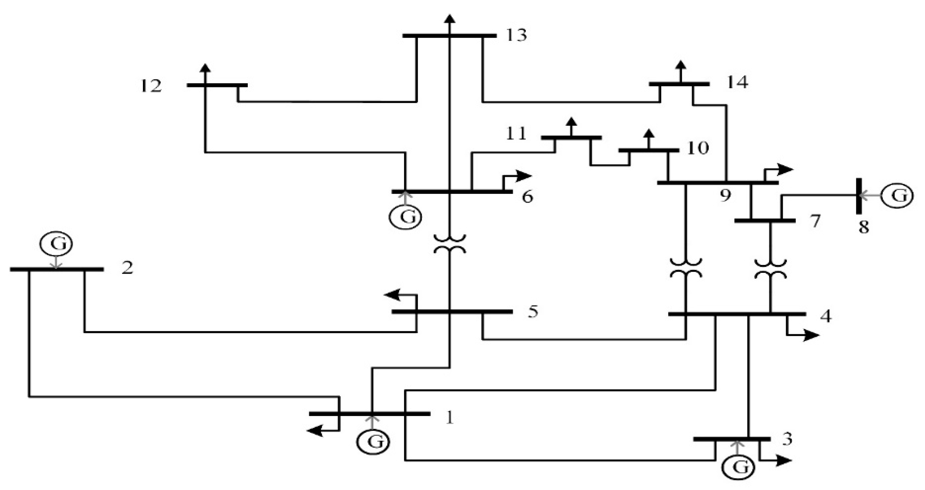
Figure 2 illustrates the IEEE 14-bus test system, which consists of five generator buses, three transformers, nine load buses, and 20 transmission lines. The bus data, limitations, and cost coefficients are presented in [119]. The transformer tap’s minimum and maximum boundaries are set to 0.9 and 1.1 p.u. The lower and upper limit voltages for all generator buses have been set at 0.94 and 1.06 p.u.
To establish an effective comparison, Table 2 and Table 3 present the detailed outcomes of the objective functions, transmission losses, and active and reactive power outputs of generators for both Cases 1 and 2. Moreover, Figure 3 illustrates the convergence behavior of the obtained fitness of the algorithms over the course of iterations on the IEEE 14-bus standard test system. As illustrated in Table 2, in terms of overall cost, both MFO and WMFO provide superior outcomes than other algorithms. For Case 2, Table 3 shows that the WMFO’s results are superior to those of other algorithms.

6.2.2. IEEE 30-Bus Test System

Figure 4 depicts a single-line diagram of the IEEE 30-bus test system. Six generators are used on buses 1, 2, 5, 8, 11, and 13, and on lines 6–9, 6–10, 4–12, and 28–27 there are four transformers installed. The branch, bus, and generator data are taken from [120]. The minimum and maximum limits of the transformer tap are adjusted to 0.9 and 1.1 p.u. The shunt VAR compensations have lower and upper values of 0.0 and 0.05 p.u. For all generator buses, the lower and upper limit voltages have been adjusted to 0.95 and 1.1 p.u.
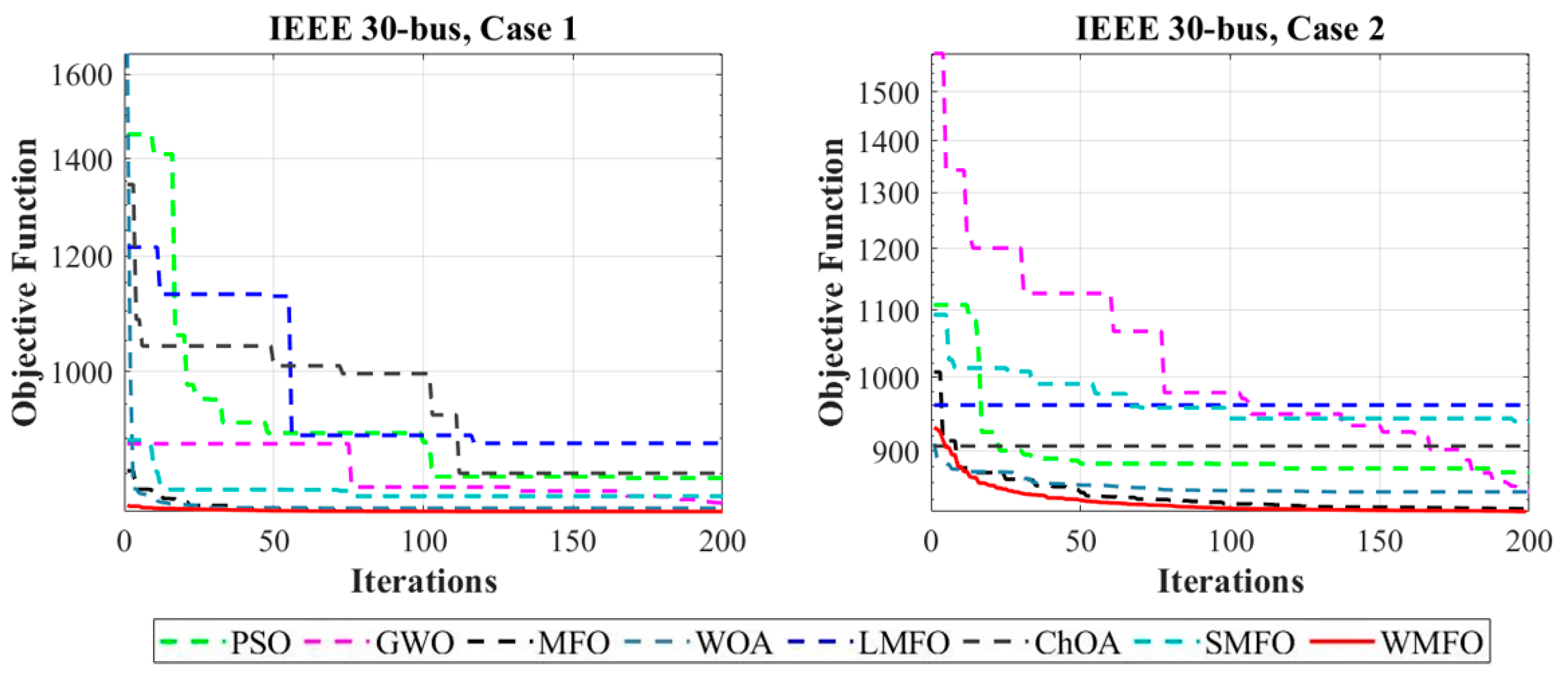
 Table 4 and Table 5 illustrate the optimal control variable values including total cost of fuel, voltage deviations, and power loss for Cases 1 and 2. Figure 5 shows the obtained fitness’ convergence trait for both Cases. It is clear to observe that WMFO provides the minimum total fuel cost of 800.603 ($/h) and 804.209 ($/h) for Case 1 and Case 2.

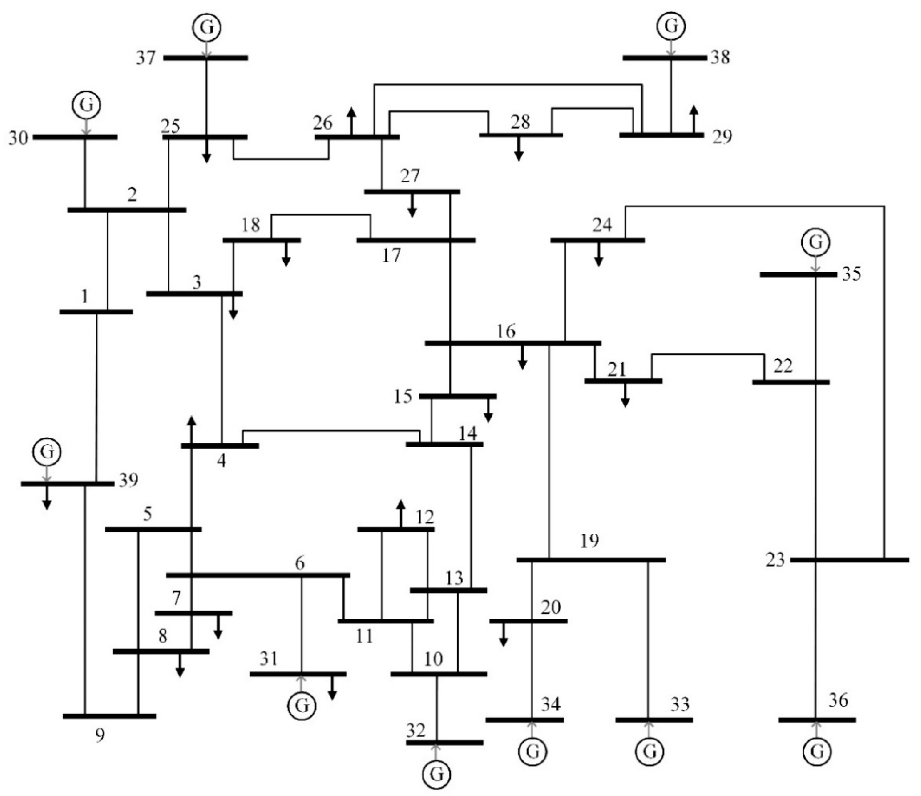
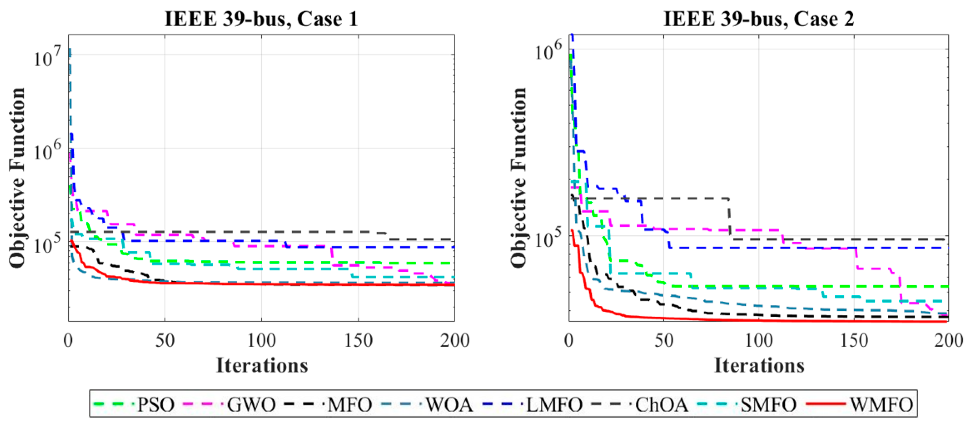
6.2.3. IEEE 39-Bus Test System

This test system contains ten generators on buses 30, 31, 32, 33, 34, 35, 36, 37, 38, and 39, and twelve transformers between buses 12–11, 12–13, 6–31, 10–32, 19–33, 20–34, 22–35, 23–36, 25–37, 2–30, 29–38, and 19–20, as shown in Figure 6. The bus data, branch data, and cost coefficients are taken from MATPOWER [117]. For all generator buses, the lower and upper limit voltages are considered to be 1.06 and 0.94. The minimum and maximum limits of the transformer tap are adjusted to 0.9 and 1.1 p.u. The tabulated results in Table 6 and Table 7 prove the superiority of the WMFO in minimizing the total fuel cost to 34,486.183 for Case 1 and 34,487.119 for Case 2. The convergence trait of WMFO, canonical MFO, and the other competitor algorithms are depicted in Figure 7.

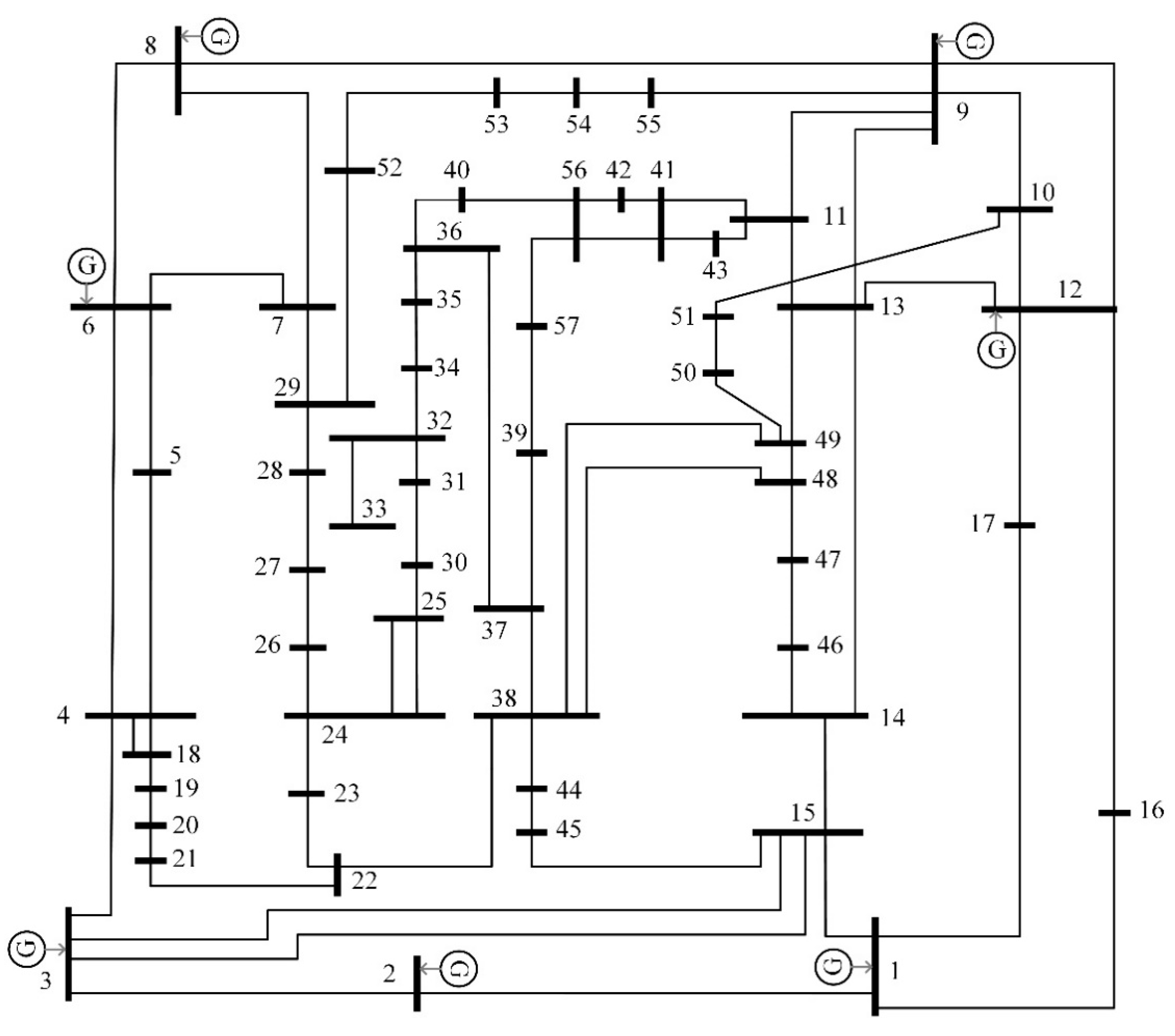
6.2.4. IEEE 57-Bus Test System

The IEEE 57-bus test system is depicted in Figure 8, and it has seven generators at the buses 1, 2, 3, 6, 8, 9, 12, and 15 branches under load tap setting transformer branches and 80 transmission lines. Shunt reactive power sources are located at buses 18, 25, and 53. The upper bounds and lower bounds of real power generations and the cost coefficients are presented in [121]. The upper and lower bounds for voltages of tap setting transformer variables and all generator buses are considered to be 1.1–0.9 in p.u. Shunt reactive power sources have maximum and lowest values of 0.0 and 0.3 in p.u. The voltages of all load buses have maximum and minimum values of 1.06 and 0.94 in p.u.
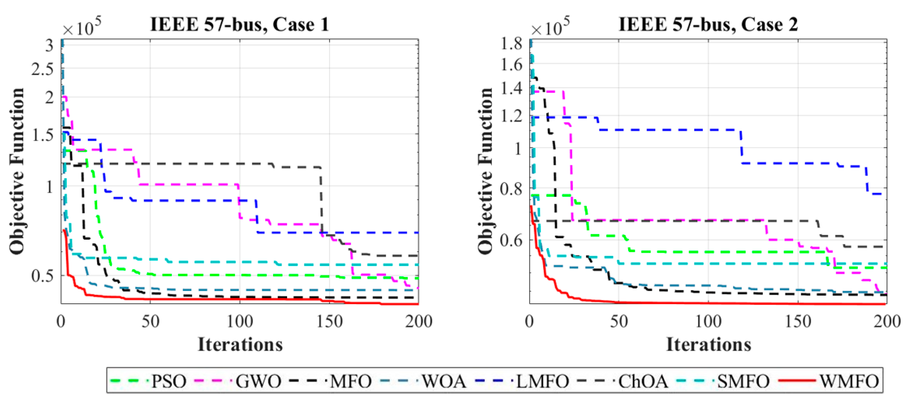
 Table 8 and Table 9 indicate that the best fuel cost values gained using the proposed WMFO are 39,359.123 ($/h) for Case 1 and 41,811.734 ($/h) for Case 2, which are significantly lower than the best fuel cost results obtained by comparative algorithms. The convergence traits of the best fuel cost acquired by the algorithms for this test system are illustrated in Figure 9.

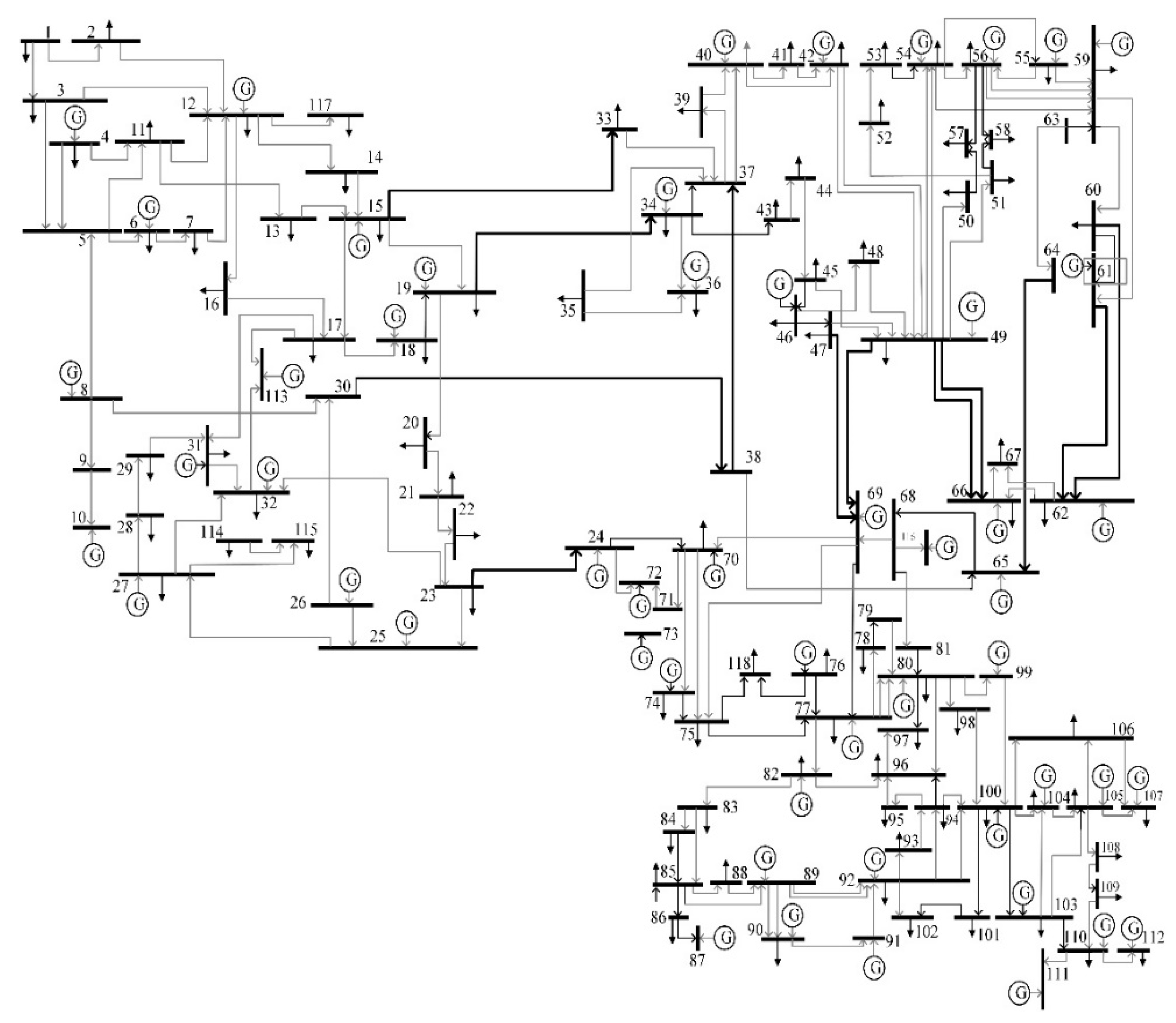
6.2.5. IEEE 118-Bus Test System

The ability of the proposed WMFO in solving a larger power system is evaluated by the IEEE 118-bus test system. The cost coefficients, branch, and bus data are taken from MATPOWER [117]. This bus test system contains 54 generators, 186 branches, 9 transformers, 2 reactors, and 12 capacitors. This system contains 129 control variables in total, as follows: there are 54 generator active powers and bus voltages are available, as well as nine transformer tap settings and twelve shunt capacitors reactive power injections. The voltage limit for all buses is 0.94 to 1.06 p.u. Transformer tap settings are tested in the range of 0.90–1.10 p.u. Shunt capacitors’ available reactive powers vary from 0 to 30 MVAR. As Cases 1 and 2 in this experiment include too many design factors, the summary of the results is reported in Table 10 and Table 11, while the detailed results of MFO, WMFO, and the proposed WMFO are tabulated in Table A1 and Table A2 in Appendix A. The results tabulated in
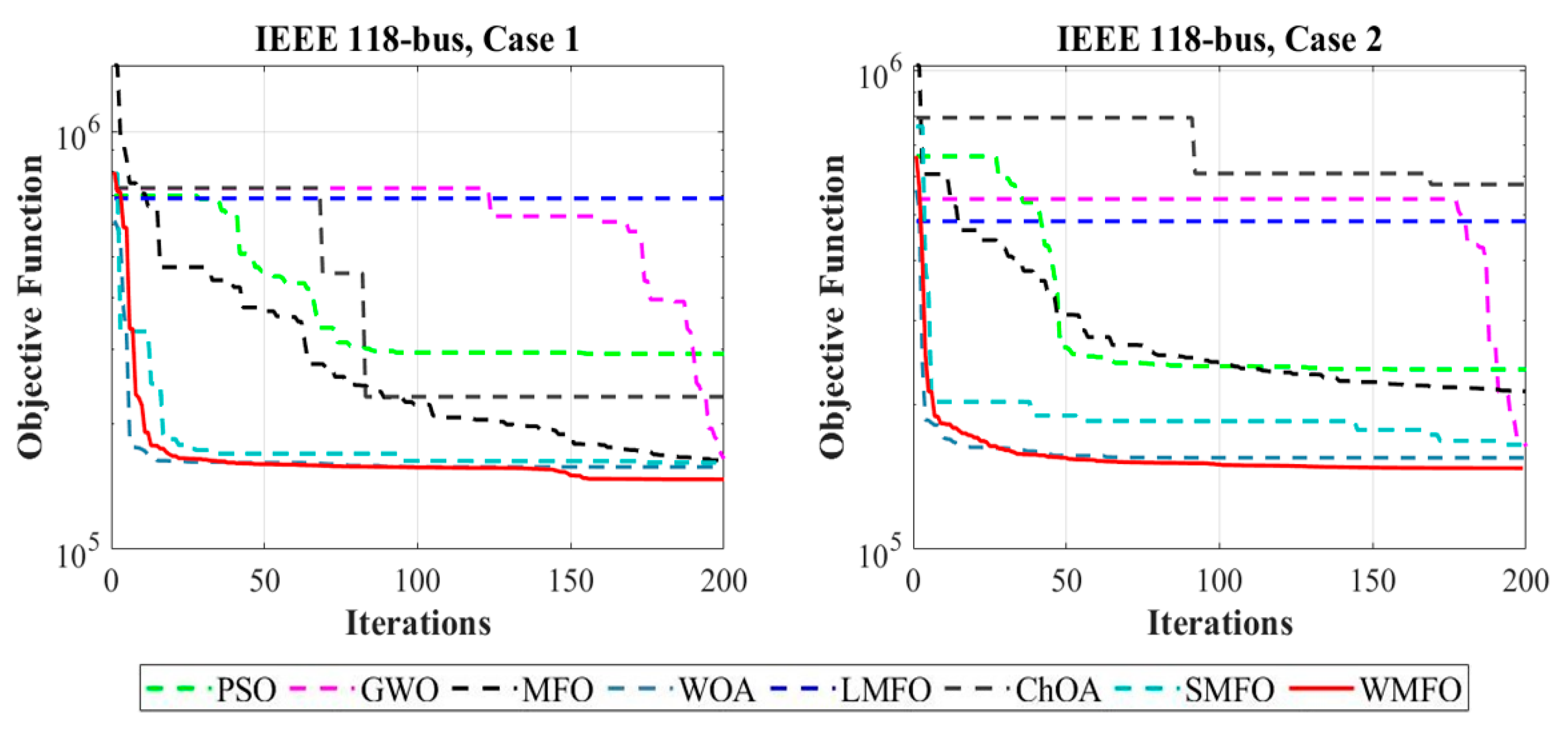
 Table 10 and Table 11 reveal that the WMFO provides the best fuel cost values. The cost value for Case 1 is 136,452.876 ($/h) and for Case 2 is 136,147.702 ($/h), which are significantly lower than the results acquired by competitor algorithms. Figure 10 and Figure 11 also show the single-line diagram of the IEEE 118-bus test system and the convergence curves of the algorithms’ acquired fitness.

7. Statistical Analysis

The algorithms are ranked based on their performance in minimizing the cost function of different OPF problems for both cases 1 and 2. The results are illustrated in the radar graph in Figure 12.
The percentage of fuel cost reduction gained by the proposed and comparative algorithms for each bus test system is illustrated in Figure 13 in comparison with the average cost for the bus test systems. It shows that the WMFO can reduce the total cost of all problems by 38.26% more than the average of competitor algorithms.

8. Conclusions and Future Works

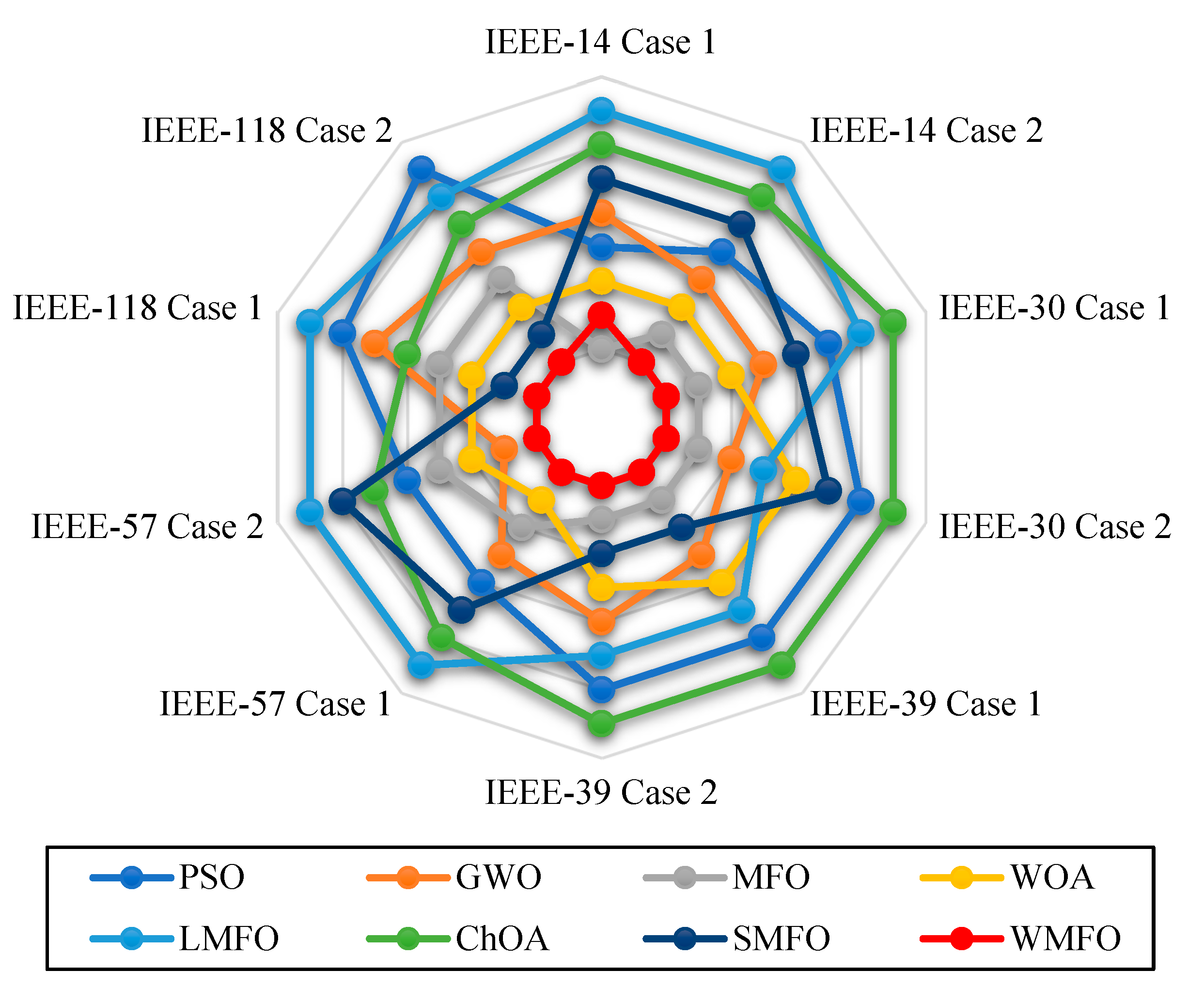
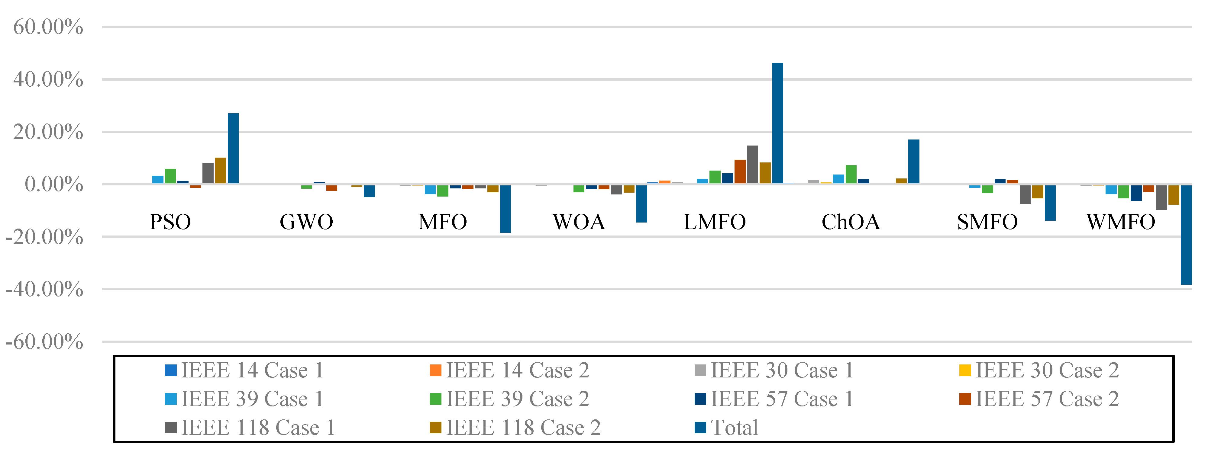
This paper proposed an effective hybridizing of whale and moth-flame optimization algorithms (WMFO) to solve the optimal power flow (OPF) problem. The population is equally partitioned among two algorithms using the population partitioning mechanism. A self-memory mechanism is defined for each search agent to preserve their best experiences and update their positions based on the average best-experienced position of the whole population. Moreover, randomized boundary handling is introduced to effectively apply the boundary limiting conditions. Furthermore, the WMFO employs a greedy selection operator to evaluate the acceptance criteria of new positions. The impact analysis on convergence curves shows that the WMFO explores the search space in the first iterations, then it keeps improving the quality of the solution in the course of iterations. This convergence behavior reveals that the WMFO inherits the exploitation of the WOA, while it takes advantage of the explorative movements of the modified MFO. The effectiveness and scalability of the proposed algorithm in solving the OPF problem have been assessed and investigated on the IEEE 14-bus, 30-bus, 39-bus, 57-bus, and 118-bus test systems to optimize the OPF’s single and multi-objective functions within the limits of the system. The obtained results are then compared against five well-known metaheuristic algorithms and two improved variations of the MFO to validate the results. The comparison of results reveals that the proposed WMFO outperforms competitor algorithms in solving single and multi-objective problems in various power system scale sizes by reducing the total cost 38.26% more than the average of the total cost gained by the competitor algorithms. The maximum amount of cost reduction compared to the average value of contender algorithms is 14,820.55 ($/h) gained by the WMFO on the IEEE 118-bus test system Case 1. Furthermore, the average amount of reduced cost gained by the WMFO on ten different OPF problems equals 33,722.24 ($/h) or 295 million dollars a year, which shows the economic viability of the proposed method in solving the OPF problem. In future research, WMFO can be employed to solve various problems in power systems such as FACTS devices and electrical load forecasting.

Author Contributions

Conceptualization, M.H.N.-S.; methodology, M.H.N.-S., H.Z. and A.F.; software, M.H.N.-S., A.F. and H.Z.; literature search, M.H.N.-S., H.Z.; validation, M.H.N.-S. and H.Z.; formal analysis, M.H.N.-S., A.F. and H.Z.; investigation, M.H.N.-S., A.F. and H.Z.; resources, M.H.N.-S., S.M., and D.O.; data curation, M.H.N.-S., A.F. and H.Z.; writing, M.H.N.-S., A.F. and H.Z.; original draft preparation, M.H.N.-S., A.F. and H.Z.; writing—review and editing, M.H.N.-S., A.F., H.Z., S.M. and D.O.; visualization, M.H.N.-S., A.F. and H.Z.; supervision, M.H.N.-S. and S.M.; project administration, M.H.N.-S. and S.M. All authors have read and agreed to the published version of the manuscript.

Funding

This research received no external funding.

Data Availability Statement

The data and code used in the research may be obtained from the corresponding author upon request.

Conflicts of Interest

The authors declare no conflict of interest.

Appendix A

Table A1 and Table A2 present the complete results of the total fuel cost (cost), power losses (ploss), and voltage deviation (VD) for Cases 1 and 2 on the IEEE-118 bus test system.
Table A1. Control variables for IEEE 118-bus test system on case 1.
DVsPSOGWOMFOWOALMFOChOASMFOWMFODVsPSOGWOMFOWOALMFOChOASMFOWMFODVsPSOGWOMFOWOALMFOChOASMFOWMFO
PG010.0064.610.0042.1255.0930.5641.8612.41PG100352.00212.36350.9028.97224.60131.85154.56123.13VG740.941.010.981.050.940.941.030.96
PG040.0037.2399.8353.8661.8414.7544.8032.27PG1030.0011.4032.1291.42112.880.0060.2124.70VG760.940.990.941.050.970.941.030.94
PG06100.0014.990.0818.9050.8656.1446.6920.95PG1040.0047.640.0044.9543.7517.1143.9678.19VG770.940.980.991.051.010.941.030.98
PG080.0039.5193.2865.0367.76100.0045.3420.95PG105100.0070.3189.3264.776.0634.7745.4457.77VG800.950.981.001.051.040.941.030.99
PG10550.00164.00354.16214.58531.54105.48241.72347.96PG107100.0056.2599.9142.4229.9658.8844.7416.53VG850.940.971.011.050.970.941.030.99
PG120.0088.06185.00105.574.9918.0373.9453.33PG110100.0071.900.0034.6223.2515.8045.196.96VG870.941.061.021.051.001.061.030.97
PG150.0021.63100.0046.0019.9736.4544.2835.70PG111136.0042.2919.6936.6492.56136.0059.2872.44VG890.940.961.061.050.970.941.031.02
PG180.0064.864.3750.9913.5823.8045.7346.25PG1120.0037.8721.7384.4117.900.0021.7236.05VG900.941.010.951.051.020.941.031.00
PG19100.0034.690.0054.7437.06100.0045.2053.02PG113100.0035.5097.0083.1194.3828.4727.090.90VG910.940.980.941.051.010.941.030.97
PG24100.0082.0999.3168.1466.2836.5244.615.78PG116100.0064.50100.0055.0130.8048.2935.893.11VG920.940.961.011.041.020.941.030.96
PG25320.00300.743.82184.34164.74213.22143.96201.05VG010.941.040.991.051.040.941.030.95VG991.060.951.061.051.060.941.030.97
PG260.00280.83267.17254.0243.61414.00166.36155.66VG040.941.041.041.051.020.941.030.97VG1001.050.991.061.051.040.951.030.97
PG27100.0046.4185.5711.9899.4748.4945.4536.28VG060.941.041.011.050.940.941.030.97VG1031.061.001.061.050.940.941.030.96
PG310.0068.742.6140.1396.700.0042.964.39VG080.941.041.021.041.030.941.030.95VG1041.061.001.051.050.970.941.030.97
PG32100.0074.67100.0046.1175.5416.2344.3171.24VG100.941.011.061.050.980.941.031.00VG1051.061.001.051.050.990.941.030.96
PG340.0070.090.0059.5693.080.0043.5516.43VG120.941.041.011.051.010.941.030.97VG1071.060.961.051.051.020.941.030.97
PG36100.0017.410.0012.2633.9684.1843.6751.16VG150.941.030.951.051.020.941.030.96VG1100.971.001.061.050.980.941.030.95
PG400.0026.450.0064.4143.930.0044.8011.68VG180.941.030.951.051.000.941.030.97VG1110.941.001.061.050.990.941.030.95
PG42100.0039.000.0047.0799.25100.0044.5352.68VG190.941.030.941.051.060.941.030.96VG1120.940.971.051.050.940.941.030.97
PG460.0027.180.0045.3414.7537.6047.4618.87VG241.060.981.061.051.000.941.030.96VG1131.061.041.001.050.971.061.030.97
PG49304.00252.5079.3039.1214.06125.87132.11153.77VG250.941.020.991.051.061.061.030.99VG1160.941.020.951.051.020.941.030.96
PG540.00131.180.0084.17127.8160.1766.5448.11VG260.940.991.051.050.980.941.030.95T (5-8)0.901.050.960.981.000.900.990.93
PG550.0073.7710.9932.2231.5765.3439.9210.04VG271.060.961.061.041.030.941.030.97T(25-26)1.100.981.101.000.980.900.990.96
PG56100.0031.1089.6011.2722.9121.8344.468.19VG311.061.041.061.051.050.941.030.97T(17-30)1.080.971.100.970.960.910.990.95
PG59255.0053.32190.0863.82220.23255.00113.21145.94VG321.061.001.061.051.040.941.030.97T(37-38)1.101.021.090.971.050.900.990.98
PG610.00135.93141.72139.13208.93154.85111.81203.45VG340.941.030.971.050.960.941.030.97T(59-63)0.900.931.080.980.980.900.990.96
PG620.0046.4016.6917.4544.1928.0245.366.64VG360.941.030.961.050.950.941.030.97T(61-64)0.901.051.101.011.020.900.990.94
PG65491.00148.41235.54256.80155.54477.67219.9982.58VG401.061.031.051.050.950.941.030.97T(65-66)1.101.081.100.981.050.900.990.94
PG660.00209.28373.1196.29100.68281.97223.00418.30VG421.060.951.041.050.970.941.030.96T(68-69)0.901.051.010.971.000.900.990.96
PG700.0044.310.0059.0563.4626.5611.863.44VG460.941.011.041.050.960.941.030.97T (80-81)0.901.041.100.971.000.900.991.03
PG72100.0044.1167.2478.4739.0018.0243.4718.93VG490.941.011.001.051.000.941.030.98QC3430.0021.770.0122.494.400.0013.383.22
PG730.0068.1899.9573.983.240.0045.2866.04VG540.941.060.971.061.040.941.030.99QC440.0018.8529.4510.5517.1214.4013.308.79
PG74100.0014.6699.9971.8672.3516.8143.9533.65VG550.941.050.961.051.010.941.030.98QC4530.0016.3128.0819.3118.2522.6113.664.34
PG7618.2841.3599.5722.9632.1592.8543.1223.57VG560.941.050.961.051.030.941.030.99QC460.0017.4530.0023.6514.2811.3513.726.12
PG77100.0046.45100.0078.4491.880.0039.4338.63VG591.061.030.941.051.040.951.030.98QC480.0012.2030.004.6014.705.2913.615.98
PG800.00215.54146.32396.90255.43119.63236.19353.31VG611.061.000.991.051.030.941.031.00QC740.0011.730.0021.506.6930.0013.013.79
PG85100.0058.260.1464.1234.8933.5241.1986.79VG621.030.981.001.051.060.941.030.99QC7930.006.0726.7419.224.820.0013.512.65
PG870.0024.567.765.8168.0133.5726.313.27VG650.991.041.061.051.060.941.030.96QC820.0018.0315.087.225.790.0012.0024.38
PG890.00158.609.2599.62283.50448.59309.44472.55VG660.940.971.021.051.031.061.030.99QC8330.006.8124.1517.9729.760.0013.693.70
PG900.0024.0383.6830.955.690.0045.231.92VG690.941.041.031.050.960.941.031.02QC1050.0027.3729.984.6120.850.0013.2810.70
PG910.0097.950.0038.5128.1975.1127.0733.07VG700.941.011.011.050.950.941.030.96QC10730.009.148.5416.3325.2230.0013.4320.65
PG920.0015.2076.9712.8549.100.0044.4014.04VG721.061.020.961.051.031.061.030.97QC1100.0010.300.003.9728.947.4713.0816.87
PG99100.0061.670.0065.2124.45100.0045.0047.50VG730.940.981.061.050.951.061.030.95
FinalResultsPSOGWOMFOWOALMFOChOASMFOWMFO
Cost($/h)163,509.345151,775.538148,925.660145,495.166173,485.645150,735.185139,808.042136,452.876
Ploss (MW)174.03688.617139.27679.658123.261126.52957.310105.637
VD(p.u.)3.4061.6161.7212.8191.4314.2121.5052.280
Table A2. Control variables for IEEE 118-bus test system on case 2.
DVsPSOGWOMFOWOALMFOChOASMFOWMFODVsPSOGWOMFOWOALMFOChOASMFOWMFODVsPSOGWOMFOWOALMFOChOASMFOWMFO
PG010.0057.8460.1743.0168.834.0645.5725.74PG100326.76110.07100.59219.25195.63238.11157.14244.89VG740.940.960.991.010.961.061.010.98
PG04100.0036.5778.2949.1428.984.5644.933.78PG1030.0046.4043.6297.8473.4416.8862.6723.28VG760.940.950.941.011.021.051.010.95
PG06100.0028.51100.0055.0673.1693.9745.3190.21PG104100.0062.830.0025.982.9311.8844.754.78VG770.940.981.001.010.991.031.010.99
PG08100.0019.96100.0069.4669.909.430.0055.55PG1050.0096.250.3633.3851.3494.5045.3939.56VG800.941.021.001.020.951.061.011.01
PG10550.0060.710.00219.72528.60422.01248.23413.30PG107100.0033.930.0067.5595.6233.7544.139.23VG850.940.971.031.010.971.041.011.00
PG12185.00115.2016.3741.1314.71180.350.0068.89PG1105.7892.71100.0081.6120.4420.5845.8913.17VG870.941.021.061.010.951.061.010.99
PG15100.0070.5479.9563.4440.7225.520.0025.01PG111136.0059.5664.0927.2751.5090.6760.8088.73VG890.941.021.021.011.051.061.011.04
PG180.0054.970.0049.7860.3945.7344.0067.91PG112100.0028.64100.0056.2599.4627.9946.4462.58VG900.940.991.041.021.001.031.010.99
PG190.0042.551.7621.5314.8241.1745.1767.25PG1130.0064.6612.1325.5688.6017.010.0017.71VG911.001.041.061.020.971.061.011.00
PG240.0075.150.1476.7058.768.0543.517.07PG1160.0031.0416.4611.9416.2861.6044.2544.25VG920.990.991.011.011.051.051.010.99
PG25320.00130.84115.65216.52236.86115.59141.8425.35VG011.041.020.981.010.961.061.010.98VG991.061.051.061.011.051.061.011.02
PG260.00238.78199.93173.8793.8131.05188.05307.37VG041.061.040.991.010.971.051.010.99VG1001.061.020.991.010.981.061.011.00
PG272.7523.980.000.0055.2443.7745.7911.52VG061.061.020.991.020.971.061.010.99VG1031.061.050.971.011.021.061.010.99
PG310.0041.530.0042.3331.1944.2847.6012.03VG080.940.960.941.020.971.061.010.98VG1041.061.030.941.010.941.061.010.99
PG32100.0036.6458.1537.0399.9631.2346.1727.29VG100.941.020.961.010.951.061.011.00VG1051.061.040.941.020.981.061.010.98
PG340.0036.1445.3374.9347.4642.7144.5640.42VG121.061.010.991.011.011.051.011.00VG1071.061.060.941.011.041.061.010.97
PG36100.0014.8094.1659.7079.2375.9345.656.24VG151.060.980.951.010.971.061.010.99VG1101.001.031.011.011.041.061.010.98
PG400.0064.46100.0013.5975.8261.4245.8310.18VG181.060.970.941.010.951.061.011.00VG1110.941.001.061.011.011.061.010.98
PG42100.0056.790.0031.0223.0763.6446.197.36VG191.060.960.941.010.951.061.010.99VG1121.061.021.011.011.041.061.010.99
PG460.005.8910.020.4842.7532.2953.497.34VG241.061.020.941.020.951.061.011.01VG1131.061.040.941.020.971.051.011.00
PG4970.0368.76180.247.4127.2710.27135.3585.59VG251.061.001.031.010.971.061.011.02VG1160.941.000.941.011.001.061.010.98
PG540.0082.430.003.98146.4479.9067.2649.55VG261.061.031.031.011.021.061.010.99T (5-8)0.900.910.900.981.041.100.990.95
PG550.0064.5994.4611.292.0958.5245.2140.42VG271.061.011.061.010.971.061.010.99T(25-26)1.101.101.011.001.081.100.990.97
PG56100.0034.3676.2466.3527.0038.5744.5810.76VG311.061.001.061.011.021.061.010.99T(17-30)0.901.001.101.021.101.100.990.97
PG59255.00193.08163.208.80249.4682.13114.8878.52VG321.060.991.031.010.981.061.010.99T(37-38)0.901.080.900.970.971.100.990.99
PG61260.0051.76116.97165.9468.27208.05115.45154.24VG341.060.961.041.021.021.061.010.98T(59-63)0.901.021.090.961.051.100.990.98
PG620.0027.1981.6552.8253.5615.1644.8922.65VG361.060.951.051.021.051.061.010.98T(61-64)0.901.051.020.961.001.010.990.96
PG650.0089.22227.27172.8428.18399.21216.37269.89VG401.061.001.061.011.041.061.011.00T(65-66)0.901.060.951.010.930.960.990.99
PG660.00379.29322.06354.0577.4444.73222.87331.40VG421.061.001.061.011.041.061.010.99T(68-69)1.101.070.901.001.091.010.990.95
PG700.0010.19100.009.8912.323.6846.3124.29VG461.060.961.021.011.011.061.010.99T (80-81)1.101.000.900.961.041.050.990.98
PG72100.0016.5913.5020.4825.3016.9843.619.61VG491.060.981.061.010.941.061.011.01QC340.0013.232.3523.2127.3817.0413.2521.88
PG730.0023.460.000.3530.1128.6244.5031.17VG540.941.051.061.011.001.061.011.00QC4430.0026.570.0022.1818.573.9713.1215.34
PG740.0067.3218.4848.2837.5427.0744.9870.85VG550.941.041.051.011.011.061.010.99QC4530.0017.1330.0022.990.6511.3513.486.91
PG76100.0028.290.000.2182.7430.5443.927.52VG560.941.041.051.011.011.061.010.99QC460.0021.5817.2024.186.6523.6413.188.27
PG77100.0066.43100.0011.3979.6354.0745.2023.82VG590.941.050.941.021.031.061.011.00QC4819.1412.3430.004.8425.988.1813.7213.25
PG80577.00111.30460.17460.7816.95453.56267.40321.42VG610.941.050.941.011.041.051.011.00QC7430.0026.2430.0013.7112.4113.0113.7524.21
PG85100.0051.76100.0060.8681.5888.3844.4136.26VG620.941.030.941.011.021.061.011.00QC7930.0014.580.017.8616.385.8513.8324.19
PG870.0013.010.625.7050.9919.850.005.42VG650.941.060.981.011.031.061.010.99QC820.002.8130.001.6526.392.9413.193.81
PG890.00531.25229.17221.43190.43594.58321.33411.41VG661.061.021.021.011.031.061.011.00QC830.0017.080.0015.0216.182.7813.424.92
PG900.0061.710.0015.0266.7929.3345.0111.87VG690.941.001.061.010.991.041.011.00QC10530.007.7319.196.0519.2722.8513.5927.63
PG91100.0060.6518.4058.2722.574.3244.021.75VG700.940.981.001.010.991.061.011.00QC10730.0011.2530.0023.1223.5214.4613.6210.45
PG920.0048.80100.0048.0066.0747.3443.994.03VG721.060.971.061.010.971.061.010.99QC1100.0010.6930.0017.104.155.7513.3411.55
PG990.0029.9097.5163.4522.8160.980.0083.21VG730.940.980.941.010.961.061.011.01
Final ResultsPSOGWOMFOWOALMFOChOASMFOWMFO
Cost($/h)162,577.805146,190.125143,148.753143,067.030159,753.193150,749.192139,773.974136,147.702
Ploss (MW)164.015125.125103.421102.091134.400131.86367.651104.699
VD(p.u.)3.2591.4821.9960.6291.6943.2630.4820.933

References

  1. Naderi, E.; Pourakbari-Kasmaei, M.; Abdi, H. An efficient particle swarm optimization algorithm to solve optimal power flow problem integrated with FACTS devices. Appl. Soft Comput. 2019, 80, 243–262. [Google Scholar] [CrossRef]
  2. Frank, S.; Steponavice, I.; Rebennack, S. Optimal power flow: A bibliographic survey. Energy Syst. 2012, 3, 221–258. [Google Scholar] [CrossRef]
  3. Burchett, R.; Happ, H.; Vierath, D. Quadratically convergent optimal power flow. IEEE Trans. Power Appar. Syst. 1984, 103, 3267–3275. [Google Scholar] [CrossRef]
  4. Habibollahzadeh, H.; Luo, G.-X.; Semlyen, A. Hydrothermal optimal power flow based on a combined linear and nonlinear programming methodology. IEEE Trans. Power Syst. 1989, 4, 530–537. [Google Scholar] [CrossRef]
  5. Torres, G.L.; Quintana, V.H. An interior-point method for nonlinear optimal power flow using voltage rectangular coordinates. IEEE Trans. Power Syst. 1998, 13, 1211–1218. [Google Scholar] [CrossRef]
  6. Santos, A.J.; Da Costa, G. Optimal-power-flow solution by Newton’s method applied to an augmented Lagrangian function. IEE Proc. Gener. Transm. Distrib. 1995, 142, 33–36. [Google Scholar] [CrossRef]
  7. Tinney, W.F.; Hart, C.E. Power flow solution by Newton’s method. IEEE Trans. Power Appar. Syst. 1967, 86, 1449–1460. [Google Scholar] [CrossRef]
  8. Ibrahim, R.A.; Ewees, A.A.; Oliva, D.; Abd Elaziz, M.; Lu, S. Improved salp swarm algorithm based on particle swarm optimization for feature selection. J. Ambient Intell. Humaniz. Comput. 2019, 10, 3155–3169. [Google Scholar] [CrossRef]
  9. Dhiman, G.; Oliva, D.; Kaur, A.; Singh, K.K.; Vimal, S.; Sharma, A.; Cengiz, K. BEPO: A novel binary emperor penguin optimizer for automatic feature selection. Knowl. Based Syst. 2021, 211, 106560. [Google Scholar] [CrossRef]
  10. Elaziz, M.A.; Abualigah, L.; Yousri, D.; Oliva, D.; Al-Qaness, M.A.; Nadimi-Shahraki, M.H.; Ewees, A.A.; Lu, S.; Ali Ibrahim, R. Boosting Atomic Orbit Search Using Dynamic-Based Learning for Feature Selection. Mathematics 2021, 9, 2786. [Google Scholar] [CrossRef]
  11. Mohmmadzadeh, H.; Gharehchopogh, F.S. An efficient binary chaotic symbiotic organisms search algorithm approaches for feature selection problems. J. Supercomput. 2021, 77, 1–43. [Google Scholar] [CrossRef]
  12. Rostami, O.; Kaveh, M. Optimal feature selection for SAR image classification using biogeography-based optimization (BBO), artificial bee colony (ABC) and support vector machine (SVM): A combined approach of optimization and machine learning. Comput. Geosci. 2021, 25, 911–930. [Google Scholar] [CrossRef]
  13. Abd Elaziz, M.; Oliva, D. Parameter estimation of solar cells diode models by an improved opposition-based whale optimization algorithm. Energy Convers. Manag. 2018, 171, 1843–1859. [Google Scholar] [CrossRef]
  14. Zamani, H.; Nadimi-Shahraki, M.H.; Gandomi, A.H. CCSA: Conscious neighborhood-based crow search algorithm for solving global optimization problems. Appl. Soft Comput. 2019, 85, 105583. [Google Scholar] [CrossRef]
  15. Rezaei, F.; Safavi, H.R.; Abd Elaziz, M.; El-Sappagh, S.H.A.; Al-Betar, M.A.; Abuhmed, T. An Enhanced Grey Wolf Optimizer with a Velocity-Aided Global Search Mechanism. Mathematics 2022, 10, 351. [Google Scholar] [CrossRef]
  16. Trojovský, P.; Dehghani, M. Pelican Optimization Algorithm: A Novel Nature-Inspired Algorithm for Engineering Applications. Sensors 2022, 22, 855. [Google Scholar] [CrossRef]
  17. Goud, B.S.; Reddy, C.; Bajaj, M.; Elattar, E.E.; Kamel, S. Power Quality Improvement Using Distributed Power Flow Controller with BWO-Based FOPID Controller. Sustainability 2021, 13, 11194. [Google Scholar] [CrossRef]
  18. Kharrich, M.; Kamel, S.; Hassan, M.H.; ElSayed, S.K.; Taha, I.B.M. An Improved Heap-Based Optimizer for Optimal Design of a Hybrid Microgrid Considering Reliability and Availability Constraints. Sustainability 2021, 13, 10419. [Google Scholar] [CrossRef]
  19. Gharehchopogh, F.S.; Farnad, B.; Alizadeh, A. A modified farmland fertility algorithm for solving constrained engineering problems. Concurr. Comput. Pract. Exp. 2021, 33, e6310. [Google Scholar] [CrossRef]
  20. Neshat, M.; Nezhad, M.M.; Abbasnejad, E.; Tjernberg, L.B.; Garcia, D.A.; Alexander, B.; Wagner, M. An evolutionary deep learning method for short-term wind speed prediction: A case study of the lillgrund offshore wind farm. arXiv 2020, arXiv:2002.09106. [Google Scholar]
  21. Amini, E.; Mehdipour, H.; Faraggiana, E.; Golbaz, D.; Mozaffari, S.; Bracco, G.; Neshat, M. Optimization Study of Hydraulic Power Take-off System for an Ocean Wave Energy Converter. arXiv 2021, arXiv:2112.09803. [Google Scholar]
  22. Zheng, Y.; Yuan, Y.; Zheng, Q.; Lei, D. A Hybrid Imperialist Competitive Algorithm for the Distributed Unrelated Parallel Machines Scheduling Problem. Symmetry 2022, 14, 204. [Google Scholar] [CrossRef]
  23. Ceylan, O.; Neshat, M.; Mirjalili, S. Cascaded H-bridge multilevel inverters optimization using adaptive grey wolf optimizer with local search. Electr. Eng. 2021, 1–15. [Google Scholar] [CrossRef]
  24. Eslami, M.; Neshat, M.; Khalid, S.A. A Novel Hybrid Sine Cosine Algorithm and Pattern Search for Optimal Coordination of Power System Damping Controllers. Sustainability 2022, 14, 541. [Google Scholar] [CrossRef]
  25. Assimi, H.; Neumann, F.; Wagner, M.; Li, X. Novelty particle swarm optimisation for truss optimisation problems. In Proceedings of the Genetic and Evolutionary Computation Conference Companion, Lille, France, 10–14 July 2021; pp. 67–68. [Google Scholar]
  26. Nadimi-Shahraki, M.H.; Taghian, S.; Mirjalili, S.; Zamani, H.; Bahreininejad, A. GGWO: Gaze Cues Learning-based Grey Wolf Optimizer and its Applications for Solving Engineering Problems. J. Comput. Sci. 2022, 101636. [Google Scholar] [CrossRef]
  27. Lyu, D.; Wang, B.; Zhang, W. Large-Scale Complex Network Community Detection Combined with Local Search and Genetic Algorithm. Appl. Sci. 2020, 10, 3126. [Google Scholar] [CrossRef]
  28. Li, X.; Wu, X.; Xu, S.; Qing, S.; Chang, P.-C. A novel complex network community detection approach using discrete particle swarm optimization with particle diversity and mutation. Appl. Soft Comput. 2019, 81, 105476. [Google Scholar] [CrossRef]
  29. Nadimi-Shahraki, M.H.; Moeini, E.; Taghian, S.; Mirjalili, S. DMFO-CD: A Discrete Moth-Flame Optimization Algorithm for Community Detection. Algorithms 2021, 14, 314. [Google Scholar] [CrossRef]
  30. Žalik, K.R.; Žalik, B. Memetic algorithm using node entropy and partition entropy for community detection in networks. Inf. Sci. 2018, 445, 38–49. [Google Scholar] [CrossRef]
  31. Goldanloo, M.J.; Gharehchopogh, F.S. A hybrid OBL-based firefly algorithm with symbiotic organisms search algorithm for solving continuous optimization problems. J. Supercomput. 2021, 78, 1–34. [Google Scholar] [CrossRef]
  32. Xie, Y.; Neumann, A.; Neumann, F. Heuristic strategies for solving complex interacting stockpile blending problem with chance constraints. arXiv 2021, arXiv:2102.05303. [Google Scholar]
  33. Asghari, K.; Masdari, M.; Gharehchopogh, F.S.; Saneifard, R. Multi-swarm and chaotic whale-particle swarm optimization algorithm with a selection method based on roulette wheel. Expert Syst. 2021, 38, e12779. [Google Scholar] [CrossRef]
  34. Dehkordi, A.A.; Sadiq, A.S.; Mirjalili, S.; Ghafoor, K.Z. Nonlinear-based Chaotic Harris Hawks Optimizer: Algorithm and Internet of Vehicles application. Appl. Soft Comput. 2021, 107574. [Google Scholar] [CrossRef]
  35. Nadimi-Shahraki, M.H.; Fatahi, A.; Zamani, H.; Mirjalili, S.; Abualigah, L.; Abd Elaziz, M. Migration-Based Moth-Flame Optimization Algorithm. Processes 2021, 9, 2276. [Google Scholar] [CrossRef]
  36. Agushaka, O.; Ezugwu, A.; Abualigah, L. Dwarf Mongoose Optimization Algorithm. Comput. Methods Appl. Mech. Eng. 2022, 391, 114570. [Google Scholar] [CrossRef]
  37. Sharma, S.; Chakraborty, S.; Saha, A.K.; Nama, S.; Sahoo, S.K. mLBOA: A Modified Butterfly Optimization Algorithm with Lagrange Interpolation for Global Optimization. Journal of Bionic Engineering 2022, 1–16. [Google Scholar] [CrossRef]
  38. Fister Jr, I.; Yang, X.-S.; Fister, I.; Brest, J.; Fister, D. A brief review of nature-inspired algorithms for optimization. arXiv 2013, arXiv:1307.4186. [Google Scholar]
  39. Holland, J.H. Genetic algorithms. Sci. Am. 1992, 267, 66–73. [Google Scholar] [CrossRef]
  40. Storn, R.; Price, K. Differential evolution–a simple and efficient heuristic for global optimization over continuous spaces. J. Glob. Optim. 1997, 11, 341–359. [Google Scholar] [CrossRef]
  41. Beyer, H.-G.; Schwefel, H.-P. Evolution strategies–a comprehensive introduction. Nat. Comput. 2002, 1, 3–52. [Google Scholar] [CrossRef]
  42. Bakirtzis, A.G.; Biskas, P.N.; Zoumas, C.E.; Petridis, V. Optimal power flow by enhanced genetic algorithm. IEEE Trans. Power Syst. 2002, 17, 229–236. [Google Scholar] [CrossRef]
  43. Zamani, H.; Nadimi-Shahraki, M.H.; Gandomi, A.H. QANA: Quantum-based avian navigation optimizer algorithm. Eng. Appl. Artif. Intell. 2021, 104, 104314. [Google Scholar] [CrossRef]
  44. Nadimi-Shahraki, M.H.; Taghian, S.; Mirjalili, S.; Faris, H. MTDE: An effective multi-trial vector-based differential evolution algorithm and its applications for engineering design problems. Appl. Soft Comput. 2020, 97, 106761. [Google Scholar] [CrossRef]
  45. Mou, X.; Shen, Z.; Liu, H.; Xv, H.; Xia, X.; Chen, S. FEM-Validated Optimal Design of Laminate Process Parameters Based on Improved Genetic Algorithm. J. Compos. Sci. 2022, 6, 21. [Google Scholar] [CrossRef]
  46. Kennedy, J.; Eberhart, R. Particle swarm optimization. In Proceedings of the ICNN’95-International Conference on Neural Networks, Perth, WA, Australia, 27 November–1 December 1995; pp. 1942–1948. [Google Scholar]
  47. Dorigo, M.; Birattari, M.; Stutzle, T. Ant colony optimization. IEEE Comput. Intell. Mag. 2006, 1, 28–39. [Google Scholar] [CrossRef]
  48. Gandomi, A.H.; Alavi, A.H. Krill herd: A new bio-inspired optimization algorithm. Commun. Nonlinear Sci. Numer. Simul. 2012, 17, 4831–4845. [Google Scholar] [CrossRef]
  49. Mirjalili, S.; Mirjalili, S.M.; Lewis, A. Grey wolf optimizer. Adv. Eng. Softw. 2014, 69, 46–61. [Google Scholar] [CrossRef] [Green Version]
  50. Khishe, M.; Mosavi, M.R. Chimp optimization algorithm. Expert Syst. Appl. 2020, 149, 113338. [Google Scholar] [CrossRef]
  51. Zamani, H.; Nadimi-Shahraki, M.H.; Gandomi, A.H. Starling murmuration optimizer: A novel bio-inspired algorithm for global and engineering optimization. Comput. Methods Appl. Mech. Eng. 2022, 392, 114616. [Google Scholar] [CrossRef]
  52. Mirjalili, S. Moth-flame optimization algorithm: A novel nature-inspired heuristic paradigm. Knowl. Based Syst. 2015, 89, 228–249. [Google Scholar] [CrossRef]
  53. Khurma, R.A.; Aljarah, I.; Sharieh, A. An Efficient Moth Flame Optimization Algorithm using Chaotic Maps for Feature Selection in the Medical Applications. In Proceedings of the ICPRAM, Valletta, Malta, 22–24 February 2020; pp. 175–182. [Google Scholar]
  54. Hassanien, A.E.; Gaber, T.; Mokhtar, U.; Hefny, H. An improved moth flame optimization algorithm based on rough sets for tomato diseases detection. Comput. Electron. Agric. 2017, 136, 86–96. [Google Scholar] [CrossRef]
  55. Gupta, D.; Ahlawat, A.K.; Sharma, A.; Rodrigues, J.J.P.C. Feature selection and evaluation for software usability model using modified moth-flame optimization. Computing 2020, 102, 1503–1520. [Google Scholar] [CrossRef]
  56. Nadimi-Shahraki, M.H.; Banaie-Dezfouli, M.; Zamani, H.; Taghian, S.; Mirjalili, S. B-MFO: A Binary Moth-Flame Optimization for Feature Selection from Medical Datasets. Computers 2021, 10, 136. [Google Scholar] [CrossRef]
  57. Abd Elaziz, M.; Ewees, A.A.; Ibrahim, R.A.; Lu, S. Opposition-based moth-flame optimization improved by differential evolution for feature selection. Math. Comput. Simul. 2020, 168, 48–75. [Google Scholar] [CrossRef]
  58. Khurma, R.A.; Aljarah, I.; Sharieh, A. A Simultaneous Moth Flame Optimizer Feature Selection Approach Based on Levy Flight and Selection Operators for Medical Diagnosis. Arab. J. Sci. Eng. 2021, 46, 8415–8440. [Google Scholar] [CrossRef]
  59. Nadimi-Shahraki, M.H.; Fatahi, A.; Zamani, H.; Mirjalili, S.; Abualigah, L. An Improved Moth-Flame Optimization Algorithm with Adaptation Mechanism to Solve Numerical and Mechanical Engineering Problems. Entropy 2021, 23, 1637. [Google Scholar] [CrossRef]
  60. Li, Y.; Zhu, X.; Liu, J. An improved moth-flame optimization algorithm for engineering problems. Symmetry 2020, 12, 1234. [Google Scholar] [CrossRef]
  61. Shan, W.; Qiao, Z.; Heidari, A.A.; Chen, H.; Turabieh, H.; Teng, Y. Double adaptive weights for stabilization of moth flame optimizer: Balance analysis, engineering cases, and medical diagnosis. Knowl. Based Syst. 2021, 214, 106728. [Google Scholar] [CrossRef]
  62. Zhang, H.; Li, R.; Cai, Z.; Gu, Z.; Heidari, A.A.; Wang, M.; Chen, H.; Chen, M. Advanced orthogonal moth flame optimization with Broyden–Fletcher–Goldfarb–Shanno algorithm: Framework and real-world problems. Expert Syst. Appl. 2020, 159, 113617. [Google Scholar] [CrossRef]
  63. Yıldız, B.S. Optimal design of automobile structures using moth-flame optimization algorithm and response surface methodology. Mater. Test. 2020, 62, 371–377. [Google Scholar] [CrossRef]
  64. Bhesdadiya, R.; Trivedi, I.N.; Jangir, P.; Jangir, N. Moth-flame optimizer method for solving constrained engineering optimization problems. In Advances in Computer and Computational Sciences; Springer: Berlin, Germany, 2018; pp. 61–68. [Google Scholar]
  65. Hussien, A.-r.; Kamel, S.; Ebeed, M.; Yu, J. A Developed Approach to Solve Economic and Emission Dispatch Problems Based on Moth-Flame Algorithm. Electr. Power Compon. Syst. 2021, 49, 94–107. [Google Scholar] [CrossRef]
  66. Mohamed, A.A.; Kamel, S.; Hassan, M.H.; Mosaad, M.I.; Aljohani, M. Optimal Power Flow Analysis Based on Hybrid Gradient-Based Optimizer with Moth–Flame Optimization Algorithm Considering Optimal Placement and Sizing of FACTS/Wind Power. Mathematics 2022, 10, 361. [Google Scholar] [CrossRef]
  67. Mirjalili, S.; Lewis, A. The whale optimization algorithm. Adv. Eng. Softw. 2016, 95, 51–67. [Google Scholar] [CrossRef]
  68. Yang, W.; Yang, Z.; Chen, Y.; Peng, Z. Modified Whale Optimization Algorithm for Multi-Type Combine Harvesters Scheduling. Machines 2022, 10, 64. [Google Scholar] [CrossRef]
  69. Cui, X.; Niu, D.; Chen, B.; Feng, J. Forecasting of Carbon Emission in China Based on Gradient Boosting Decision Tree Optimized by Modified Whale Optimization Algorithm. Sustainability 2021, 13, 12302. [Google Scholar] [CrossRef]
  70. Chakraborty, S.; Sharma, S.; Saha, A.K.; Saha, A. A novel improved whale optimization algorithm to solve numerical optimization and real-world applications. Artif. Intell. Rev. 2022, 1–112. [Google Scholar] [CrossRef]
  71. Chakraborty, S.; Sharma, S.; Saha, A.K.; Chakraborty, S. SHADE–WOA: A metaheuristic algorithm for global optimization. Appl. Soft Comput. 2021, 113, 107866. [Google Scholar] [CrossRef]
  72. Brodzicki, A.; Piekarski, M.; Jaworek-Korjakowska, J. The Whale Optimization Algorithm Approach for Deep Neural Networks. Sensors 2021, 21, 8003. [Google Scholar] [CrossRef]
  73. Chakraborty, S.; Saha, A.K.; Sharma, S.; Chakraborty, R.; Debnath, S. A hybrid whale optimization algorithm for global optimization. J. Ambient Intell. Humaniz. Comput. 2021, 1–37. [Google Scholar] [CrossRef]
  74. Rajendran, S.; Čep, R.; Narayanan, R.C.; Pal, S.; Kalita, K. A Conceptual Comparison of Six Nature-Inspired Metaheuristic Algorithms in Process Optimization. Processes 2022, 10, 197. [Google Scholar] [CrossRef]
  75. Xiang, X.; Ma, X.; Ma, Z.; Ma, M. Operational Carbon Change in Commercial Buildings under the Carbon Neutral Goal: A LASSO–WOA Approach. Buildings 2022, 12, 54. [Google Scholar] [CrossRef]
  76. Li, Z.; Zhou, Y.; Zhang, S.; Song, J. Lévy-flight moth-flame algorithm for function optimization and engineering design problems. Math. Probl. Eng. 2016, 2016, 1423930. [Google Scholar] [CrossRef] [Green Version]
  77. Chen, C.; Wang, X.; Yu, H.; Wang, M.; Chen, H. Dealing with multi-modality using synthesis of Moth-flame optimizer with sine cosine mechanisms. Math. Comput. Simul. 2021, 188, 291–318. [Google Scholar] [CrossRef]
  78. Ghasemi, M.; Ghavidel, S.; Ghanbarian, M.M.; Massrur, H.R.; Gharibzadeh, M. Application of imperialist competitive algorithm with its modified techniques for multi-objective optimal power flow problem: A comparative study. Inf. Sci. 2014, 281, 225–247. [Google Scholar] [CrossRef]
  79. Momoh, J.A.; Adapa, R.; El-Hawary, M. A review of selected optimal power flow literature to 1993. I. Nonlinear and quadratic programming approaches. IEEE Trans. Power Syst. 1999, 14, 96–104. [Google Scholar] [CrossRef]
  80. Bottero, M.; Galiana, F.; Fahmideh-Vojdani, A. Economic dispatch using the reduced hessian. IEEE Trans. Power Appar. Syst. 1982, 101, 3679–3688. [Google Scholar] [CrossRef]
  81. Niknam, T.; Narimani, M.R.; Azizipanah-Abarghooee, R. A new hybrid algorithm for optimal power flow considering prohibited zones and valve point effect. Energy Convers. Manag. 2012, 58, 197–206. [Google Scholar] [CrossRef]
  82. Ebeed, M.; Kamel, S.; Jurado, F. Optimal power flow using recent optimization techniques. In Classical and Recent Aspects of Power System Optimization; Elsevier: Amsterdam, The Netherlands, 2018; pp. 157–183. [Google Scholar]
  83. Abido, M.A. Optimal power flow using particle swarm optimization. Int. J. Electr. Power Energy Syst. 2002, 24, 563–571. [Google Scholar] [CrossRef]
  84. Bouktir, T.; Slimani, L. Optimal power flow of the algerian electrical network using an ant colony optimization method. Leonardo J. Sci. 2005, 6, 43–57. [Google Scholar]
  85. Li, Q. Shuffled frog leaping algorithm based optimal reactive power flow. In Proceedings of the 2009 International Symposium on Computer Network and Multimedia Technology, Wuhan, China, 18–20 December 2009; pp. 1–4. [Google Scholar]
  86. El Ela, A.; Abido, M.; Spea, S. Optimal power flow using differential evolution algorithm. Electr. Power Syst. Res. 2010, 80, 878–885. [Google Scholar] [CrossRef]
  87. Roy, P.; Ghoshal, S.; Thakur, S. Multi-objective optimal power flow using biogeography-based optimization. Electr. Power Compon. Syst. 2010, 38, 1406–1426. [Google Scholar] [CrossRef]
  88. Duman, S.; Güvenç, U.; Sönmez, Y.; Yörükeren, N. Optimal power flow using gravitational search algorithm. Energy Convers. Manag. 2012, 59, 86–95. [Google Scholar] [CrossRef]
  89. Herbadji, O.; Nadhir, K.; Slimani, L.; Bouktir, T. Optimal power flow with emission controlled using firefly algorithm. In Proceedings of the 2013 5th International Conference on Modeling, Simulation and Applied Optimization (ICMSAO), Hammamet, Tunisia, 28–30 April 2013; pp. 1–6. [Google Scholar]
  90. Bouchekara, H.; Abido, M.; Boucherma, M. Optimal power flow using teaching-learning-based optimization technique. Electr. Power Syst. Res. 2014, 114, 49–59. [Google Scholar] [CrossRef]
  91. El-Fergany, A.A.; Hasanien, H.M. Single and multi-objective optimal power flow using grey wolf optimizer and differential evolution algorithms. Electr. Power Compon. Syst. 2015, 43, 1548–1559. [Google Scholar] [CrossRef]
  92. Trivedi, I.N.; Jangir, P.; Parmar, S.A. Optimal power flow with enhancement of voltage stability and reduction of power loss using ant-lion optimizer. Cogent Eng. 2016, 3, 1208942. [Google Scholar] [CrossRef]
  93. Bentouati, B.; Chaib, L.; Chettih, S. Optimal power flow using the moth flam optimizer: A case study of the Algerian power system. Indones. J. Electr. Eng. Comput. Sci. 2016, 1, 431–445. [Google Scholar] [CrossRef]
  94. Saha, A.; Bhattacharya, A.; Das, P.; Chakraborty, A.K. Crow search algorithm for solving optimal power flow problem. In Proceedings of the 2017 Second International Conference on Electrical, Computer and Communication Technologies (ICECCT), Coimbatore, Tamil Nadu, 22–24 April 2017; pp. 1–8. [Google Scholar]
  95. El-Fergany, A.A.; Hasanien, H.M. Salp swarm optimizer to solve optimal power flow comprising voltage stability analysis. Neural Comput. Appl. 2020, 32, 5267–5283. [Google Scholar] [CrossRef]
  96. Mostafa, A.; Ebeed, M.; Kamel, S.; Abdel-Moamen, M. Optimal Power Flow Solution Using Levy Spiral Flight Equilibrium Optimizer With Incorporating CUPFC. IEEE Access 2021, 9, 69985–69998. [Google Scholar] [CrossRef]
  97. Farhat, M.; Kamel, S.; Atallah, A.M.; Khan, B. Optimal power flow solution based on jellyfish search optimization considering uncertainty of renewable energy sources. IEEE Access 2021, 9, 100911–100933. [Google Scholar] [CrossRef]
  98. Akdag, O. A Improved Archimedes Optimization Algorithm for multi/single-objective Optimal Power Flow. Electr. Power Syst. Res. 2022, 206, 107796. [Google Scholar] [CrossRef]
  99. Khaled, U.; Eltamaly, A.M.; Beroual, A. Optimal Power Flow Using Particle Swarm Optimization of Renewable Hybrid Distributed Generation. Energies 2017, 10, 1013. [Google Scholar] [CrossRef] [Green Version]
  100. Sivasubramani, S.; Swarup, K. Multi-objective harmony search algorithm for optimal power flow problem. Int. J. Electr. Power Energy Syst. 2011, 33, 745–752. [Google Scholar] [CrossRef]
  101. Vo, D.N.; Schegner, P. An improved particle swarm optimization for optimal power flow. In Meta-Heuristics Optimization Algorithms in Engineering, Business, Economics, and Finance; IGI Global: New York, NY, USA, 2013; pp. 1–40. [Google Scholar]
  102. Sinsuphan, N.; Leeton, U.; Kulworawanichpong, T. Optimal power flow solution using improved harmony search method. Appl. Soft Comput. 2013, 13, 2364–2374. [Google Scholar] [CrossRef]
  103. Ghasemi, M.; Ghavidel, S.; Rahmani, S.; Roosta, A.; Falah, H. A novel hybrid algorithm of imperialist competitive algorithm and teaching learning algorithm for optimal power flow problem with non-smooth cost functions. Eng. Appl. Artif. Intell. 2014, 29, 54–69. [Google Scholar] [CrossRef]
  104. Radosavljević, J.; Klimenta, D.; Jevtić, M.; Arsić, N. Optimal power flow using a hybrid optimization algorithm of particle swarm optimization and gravitational search algorithm. Electr. Power Compon. Syst. 2015, 43, 1958–1970. [Google Scholar] [CrossRef]
  105. Bai, W.; Eke, I.; Lee, K.Y. An improved artificial bee colony optimization algorithm based on orthogonal learning for optimal power flow problem. Control Eng. Pract. 2017, 61, 163–172. [Google Scholar] [CrossRef]
  106. Daqaq, F.; Ellaia, R.; Ouassaid, M. Multiobjective backtracking search algorithm for solving optimal power flow. In Proceedings of the 2017 International Conference on Electrical and Information Technologies (ICEIT), Rabat, Morocco, 15–18 November 2017; pp. 1–6. [Google Scholar]
  107. Li, S.; Gong, W.; Wang, L.; Yan, X.; Hu, C. Optimal power flow by means of improved adaptive differential evolution. Energy 2020, 198, 117314. [Google Scholar] [CrossRef]
  108. Nadimi-Shahraki, M.H.; Taghian, S.; Mirjalili, S. An improved grey wolf optimizer for solving engineering problems. Expert Syst. Appl. 2021, 166, 113917. [Google Scholar] [CrossRef]
  109. Khunkitti, S.; Siritaratiwat, A.; Premrudeepreechacharn, S. Multi-Objective Optimal Power Flow Problems Based on Slime Mould Algorithm. Sustainability 2021, 13, 7448. [Google Scholar] [CrossRef]
  110. Meng, A.; Zeng, C.; Wang, P.; Chen, D.; Zhou, T.; Zheng, X.; Yin, H. A high-performance crisscross search based grey wolf optimizer for solving optimal power flow problem. Energy 2021, 225, 120211. [Google Scholar] [CrossRef]
  111. Abd El-sattar, S.; Kamel, S.; Ebeed, M.; Jurado, F. An improved version of salp swarm algorithm for solving optimal power flow problem. Soft Comput. 2021, 25, 4027–4052. [Google Scholar] [CrossRef]
  112. Nadimi-Shahraki, M.H.; Taghian, S.; Mirjalili, S.; Abualigah, L.; Abd Elaziz, M.; Oliva, D. EWOA-OPF: Effective Whale Optimization Algorithm to Solve Optimal Power Flow Problem. Electronics 2021, 10, 2975. [Google Scholar] [CrossRef]
  113. Kahraman, H.T.; Akbel, M.; Duman, S. Optimization of Optimal Power Flow Problem Using Multi-Objective Manta Ray Foraging Optimizer. Appl. Soft Comput. 2021, 108334. [Google Scholar] [CrossRef]
  114. Alsac, O.; Stott, B. Optimal load flow with steady-state security. IEEE Trans. Power Appar. Syst. 1974, 93, 745–751. [Google Scholar] [CrossRef] [Green Version]
  115. Gharehchopogh, F.S.; Gholizadeh, H. A comprehensive survey: Whale Optimization Algorithm and its applications. Swarm Evol. Comput. 2019, 48, 1–24. [Google Scholar] [CrossRef]
  116. Chakraborty, S.; Saha, A.K.; Chakraborty, R.; Saha, M. An enhanced whale optimization algorithm for large scale optimization problems. Knowl. Based Syst. 2021, 233, 107543. [Google Scholar] [CrossRef]
  117. Zimmerman, R.; Murillo-Sanchez, C. Matpower (Version 7.0). 2019. Available online: https://zenodoorg/record/4074135#Yc6JdlkRWNI (accessed on 15 October 2021).
  118. Awad, N.; Ali, M.; Liang, J.; Qu, B.; Suganthan, P. Problem Definitions and Evaluation Criteria for the CEC 2017 Special Sessionand Competition on Single Objective Bound Constrained Real-Parameter Numerical Optimization; Technical Report; Nanyang Technological University: Singapore, 20 November 2016. [Google Scholar]
  119. Turkay, B.E.; Cabadag, R.I. Optimal power flow solution using particle swarm optimization algorithm. In Proceedings of the Eurocon 2013, Zagreb, Croatia, 1–4 July 2013; pp. 1418–1424. [Google Scholar]
  120. Zimmerman, R.D.; Murillo-Sánchez, C.E.; Thomas, R.J. MATPOWER: Steady-state operations, planning, and analysis tools for power systems research and education. IEEE Trans. Power Syst. 2010, 26, 12–19. [Google Scholar] [CrossRef] [Green Version]
  121. Vaisakh, K.; Srinivas, L. Evolving ant direction differential evolution for OPF with non-smooth cost functions. Eng. Appl. Artif. Intell. 2011, 24, 426–436. [Google Scholar] [CrossRef]
Figure 1. The convergence curves of algorithms in solving CEC benchmark functions.
Electronics 11 00831 g001
Figure 2. The one-line diagram for the IEEE 14-bus system.
Electronics 11 00831 g002
Figure 3. Convergence curves for the IEEE 14-bus test system.
Electronics 11 00831 g003
Figure 4. The one-line diagram for the IEEE 30-bus test system.
Electronics 11 00831 g004
Figure 5. Convergence curves for the IEEE 30-bus test system.
Electronics 11 00831 g005
Figure 6. The one-line diagram for the IEEE 39-bus test system.
Electronics 11 00831 g006
Figure 7. Convergence curves for the IEEE 39-bus test system.
Electronics 11 00831 g007
Figure 8. The one-line diagram for the IEEE 57-bus test system.
Electronics 11 00831 g008
Figure 9. Convergence curves for the IEEE 57-bus test system.
Electronics 11 00831 g009
Figure 10. The one-line diagram for IEEE 118-bus test system.
Electronics 11 00831 g010
Figure 11. Convergence curves for the IEEE 118-bus test system.
Electronics 11 00831 g011
Figure 12. The rank of algorithms in solving the OPF problems.
Electronics 11 00831 g012
Figure 13. The percentage of cost reduction in comparison with the average cost of each bus test system.
Electronics 11 00831 g013
Table 1. Parameter of the comparative algorithms.
AlgorithmParameter Settings
PSOc1 = c2 = 2
KHVf = 0.02, Dmax = 0.005, Nmax = 0.01, Sr = 0.
GWOa linearly decreases from 2 to 0.
MFOa decreases linearly from −1 to −2, b = 1.
WOAα parameter is linearly decreased from 2 to 0, b = 1.
LMFOv and µ are normal distributions, β = 1.5, Г is the gamma function.
ChOAf parameter is decreased linearly from 2 to 0.
SMFOr4 = random number between interval (0, 1).
WMFOα is decreased linearly from 2 to 0, b = 1.
Table 2. Control variables for the IEEE 14-bus test system on case 1.
DVsPSOGWOMFOWOALMFOChOASMFOWMFO
PG1 (MW)195.499191.895194.443193.935215.178189.794206.344194.365
PG2 (MW)31.97737.65536.72935.93734.07135.85334.56036.778
PG3 (MW)40.73315.80929.01436.0130.00041.1950.00028.834
PG6 (MW)0.00021.3330.0000.9330.0000.0000.0000.011
PG8 (MW)0.0001.9568.0371.44522.2402.32629.1218.233
VG1 (p.u)1.0601.0601.0601.0601.0351.0601.0601.060
VG2 (p.u)1.0401.0391.0391.0401.0121.0471.0391.039
VG3 (p.u)1.0121.0061.0151.0070.9531.0151.0031.015
VG6 (p.u)1.0601.0131.0601.0311.0601.0601.0411.060
VG8 (p.u)1.0601.0561.0601.0521.0600.9401.0351.060
T11(4–7) (p.u)1.0390.9851.0031.0020.9461.1001.0641.003
T12(4–9) (p.u)0.9001.0190.9001.1001.0581.1001.0470.903
T15(5–6) (p.u)0.9001.0260.9720.9700.9000.9000.9570.971
QC14 (MVAR)0.0000.0000.0000.0000.0000.0000.0000.000
Cost ($/h)8095.6428100.9888078.6598087.2708162.0538142.1588122.1228078.679
Ploss (MW)9.2099.6489.2239.26212.48910.16811.0269.221
VD (p.u)0.2780.1180.3560.1080.2390.2640.1150.354
Table 3. Control variables for the IEEE 14-bus test system on case 2.
DVsPSOGWOMFOWOALMFOChOASMFOWMFO
PG1 (MW)205.123184.105194.901189.739190.829204.696182.242195.220
PG2 (MW)32.77734.04136.79731.96058.71538.49534.56036.878
PG3 (MW)31.41620.64529.82432.8470.0001.6550.00029.290
PG6 (MW)0.0007.1090.0000.0610.00025.6370.0000.000
PG8 (MW)0.00021.7496.82813.21120.1010.19129.1216.989
VG1 (p.u)1.0601.0601.0601.0531.0601.0601.0601.060
VG2 (p.u)1.0401.0381.0401.0301.0391.0391.0391.040
VG3 (p.u)1.0011.0071.0101.0080.9880.9741.0031.010
VG6 (p.u)1.0471.0151.0151.0211.0601.0601.0411.015
VG8 (p.u)1.0601.0081.0041.0401.0601.0601.0351.008
T11(4–7) (p.u)0.9131.0451.0251.0731.0391.1001.0641.031
T12(4–9) (p.u)1.1000.9160.9400.9830.9300.9001.0470.941
T15(5–6) (p.u)0.9060.9571.0030.9950.9600.9000.9571.002
QC14 (MVAR)0.0000.0000.0000.0000.0000.0000.0000.000
Cost ($/h)8103.6098100.7018082.3928095.6778227.7488143.1738122.1228082.128
Ploss (MW)10.3178.6499.3498.81710.64511.67411.0269.379
VD (p.u)0.1940.0580.0600.0700.2920.1990.1150.062
Table 4. Control variables for the IEEE 30-bus test system on case 1.
DVsPSOGWOMFOWOALMFOChOASMFOWMFO
PG1 (MW)185.334170.079177.281181.154166.251197.128180.892177.196
PG2 (MW)50.78753.23548.72548.85245.59727.44538.39648.833
PG5 (MW)19.95623.96521.49523.65025.90516.87622.19121.298
PG8 (MW)10.00018.64121.37516.62614.27819.48418.94520.975
PG11 (MW)16.32711.60411.59810.28219.34620.93412.47412.022
PG13 (MW)12.00014.95712.00012.33821.62412.77020.00812.142
VG1 (p.u)1.1001.0641.0831.0831.0661.0591.0721.082
VG2 (p.u)1.0641.0471.0641.0651.0331.0481.0531.064
VG5 (p.u)1.0201.0141.0321.0320.9550.9901.0191.032
VG8 (p.u)0.9961.0221.0361.0310.9900.9781.0201.036
VG11 (p.u)0.9501.0871.0821.0961.0981.0411.0771.095
VG13 (p.u)1.0531.0501.0591.0601.0671.0381.0371.054
T11(6–9) (p.u)1.1000.9591.0421.0261.0740.9121.0291.052
T12(6–10) (p.u)0.9001.0290.9001.0250.9130.9960.9970.919
T15(4–12) (p.u)1.1001.0660.9800.9870.9391.0300.9700.977
T36(28–27) (p.u)0.9300.9530.9711.0160.9590.9440.9790.971
QC10 (MVAR)5.0000.3580.9692.8291.8032.4950.3493.336
QC12 (MVAR)0.0004.1250.0003.4234.7932.4100.7610.214
QC15 (MVAR)0.0002.5990.0002.8042.1683.8290.5664.409
QC17 (MVAR)5.0001.6735.0000.7901.6314.8390.2184.705
QC20 (MVAR)5.0004.1985.0001.7170.8402.4570.9102.777
QC21 (MVAR)0.0000.8940.0002.0302.7382.5561.1253.222
QC23 (MVAR)0.5210.9345.0003.2531.1322.4460.0973.011
QC24 (MVAR)1.2111.2454.9270.7581.1781.0230.6193.917
QC29 (MVAR)0.0002.3482.2693.6051.5673.2150.3262.032
Cost ($/h)806.917803.375800.647801.883812.235818.495806.361800.603
Ploss (MW)11.0049.0829.0759.5029.60111.2369.5069.066
VD (p.u)0.5480.3460.8800.4960.3630.2380.3450.875
Table 5. Control variables for the IEEE 30-bus test system on case 2.
DVsPSOGWOMFOWOALMFOChOASMFOWMFO
PG1 (MW)173.480174.013173.985168.666171.232155.248178.513175.843
PG2 (MW)43.02646.95949.52344.51438.97557.23146.09449.016
PG5 (MW)15.00017.42421.80417.43022.79222.09716.83421.631
PG8 (MW)35.00023.67624.16526.33034.99615.66312.69921.454
PG11 (MW)15.04510.32111.40214.30911.63612.24517.60612.524
PG13(MW)12.00020.91512.34421.75613.38629.27422.14912.888
VG1 (p.u)1.0611.0421.0371.0311.0881.0951.0311.037
VG2 (p.u)1.0411.0171.0221.0111.0631.0651.0191.022
VG5 (p.u)0.9651.0061.0171.0130.9851.0321.0131.018
VG8 (p.u)0.9991.0071.0051.0111.0041.0381.0111.005
VG11 (p.u)1.0211.0871.0150.9991.0291.1001.0211.022
VG13 (p.u)1.0040.9970.9911.0340.9740.9981.0320.988
T11(6–9) (p.u)0.9821.0791.0280.9440.9941.0090.9741.038
T12(6–10) (p.u)0.9340.9000.9020.9640.9441.1000.9940.909
T15(4–12) (p.u)0.9000.9370.9580.9990.9690.9750.9570.945
T36(28–27) (p.u)0.9100.9520.9530.9620.9260.9640.9570.967
QC10 (MVAR)5.0002.5894.9821.4101.1330.7102.6204.425
QC12 (MVAR)1.5421.9395.0003.9101.6391.2872.3374.302
QC15 (MVAR)0.0003.9415.0000.9680.3281.1491.7654.366
QC17 (MVAR)2.5813.1950.0002.7213.7661.8440.1743.383
QC20(MVAR)5.0002.2305.0003.9060.0620.9922.3054.971
QC21 (MVAR)0.0000.7065.0003.8124.2573.7961.7484.720
QC23 (MVAR)0.0000.8864.9713.2414.4691.6582.2204.716
QC24 (MVAR)0.5001.8065.0002.3011.2643.8022.1494.960
QC29 (MVAR)0.0001.4480.7262.9954.9990.1261.8882.335
Cost ($/h)810.931807.675804.289809.505809.345813.642810.816804.209
Ploss (MW)10.1519.9089.8229.6049.6178.35710.4969.956
VD (p.u)0.2410.1560.0970.1530.3550.3750.1910.099
Table 6. Control variables for the IEEE 39-bus test system on case 1.
DVsPSOGWOMFOWOALMFOChOASMFOWMFO
PG30 (MW)350.000299.173350.000257.596323.881200.843311.593349.822
PG32 (MW)800.000621.557550.354503.557799.727572.434473.799555.955
PG33 (MW)300.000466.940542.065460.115300.000593.647692.449554.105
PG34 (MW)650.000604.773536.948513.761328.112250.000591.664532.170
PG35 (MW)300.000626.021550.194586.473587.869750.000458.573572.003
PG36 (MW)523.141412.707563.518703.548569.564495.903524.071551.385
PG37 (MW)700.000586.306700.000635.870691.991700.000632.776699.703
PG38 (MW)900.000859.885899.994833.644900.000837.224828.653864.790
PG39 (MW)1200.0001185.663940.2771195.7881111.9161200.0001066.161957.922
VG30 (p.u)0.9401.0291.0381.0490.9961.0601.0591.028
VG31 (p.u)1.0600.9810.9401.0371.0600.9401.0590.988
VG32 (p.u)1.0601.0261.0501.0480.9400.9671.0591.007
VG33 (p.u)0.9400.9811.0331.0410.9411.0601.0591.010
VG34 (p.u)1.0601.0190.9911.0520.9401.0601.0591.036
VG35 (p.u)0.9400.9971.0601.0280.9400.9401.0591.024
VG36 (p.u)0.9401.0061.0531.0480.9400.9401.0591.027
VG37 (p.u)1.0600.9970.9851.0491.0201.0601.0591.030
VG38 (p.u)1.0601.0071.0601.0361.0601.0601.0591.038
VG39 (p.u)0.9961.0541.0111.0431.0601.0601.0591.020
T(12–11) (p.u)1.1000.9660.9811.0041.1000.9811.0061.024
T(12–13) (p.u)0.9860.9261.0241.0251.1001.1001.0071.049
T(6–31) (p.u)0.9001.0471.0550.9990.9881.1000.9921.008
T(10–32) (p.u)0.9001.0030.9470.9931.0971.1001.0120.997
T(19–33) (p.u)1.1001.0811.0121.0391.1000.9001.0081.035
T(20–34) (p.u)0.9001.0561.1001.0001.1001.0211.0011.042
T(22–35) (p.u)1.1001.0530.9641.0211.1001.1001.0131.010
T(23–36) (p.u)1.1001.0680.9841.0071.1001.1000.9981.020
T(25–37) (p.u)1.0121.0981.0941.0411.1001.0150.9921.053
T(2–30) (p.u)1.1001.0371.0140.9991.1001.0051.0171.033
T(29–38) (p.u)1.0261.0521.0060.9961.0821.1001.0081.025
T(19–20) (p.u)1.1000.9690.9621.0331.0620.9001.0100.958
QC29 (MVAR)0.0000.0000.0000.0000.0000.0000.0000.000
Cost ($/h)36,981.45235,808.00834,492.31535,922.54436,563.13637,126.97735,341.99434,486.183
Ploss (MW)51.40141.32052.64644.02048.15146.76043.92449.901
VD (p.u)1.0700.8970.7780.7281.1020.8661.1420.756
Table 7. Control variables for the IEEE 39-bus test system on case 2.
DVsPSOGWOMFOWOALMFOChOASMFOWMFO
PG30 (MW)100.000297.380348.903292.284138.518109.618313.654349.732
PG32 (MW)300.000704.308552.833569.712476.085566.034632.536560.992
PG33 (MW)750.000641.764523.129596.531300.000750.000567.150542.973
PG34 (MW)650.000634.137523.843579.320650.000250.000586.266555.768
PG35 (MW)387.945411.939509.422588.745750.000667.111578.945543.045
PG36 (MW)750.000570.735485.428629.124750.000750.000581.488561.926
PG37 (MW)700.000687.822692.822626.683700.000700.000538.703699.785
PG38 (MW)900.000738.345879.590698.947900.000566.939889.166850.778
PG39 (MW)1200.0001101.3081114.1551064.5041200.0001200.000957.452974.999
VG30 (p.u)0.9781.0510.9511.0600.9400.9401.0501.014
VG31 (p.u)0.9400.9421.0601.0601.0600.9401.0461.036
VG32 (p.u)0.9400.9581.0251.0370.9400.9401.0510.991
VG33 (p.u)0.9400.9571.0601.0600.9620.9401.0551.025
VG34 (p.u)0.9400.9441.0601.0600.9400.9401.0571.009
VG35 (p.u)0.9401.0051.0601.0310.9400.9401.0491.022
VG36 (p.u)0.9400.9620.9641.0570.9400.9401.0491.001
VG37 (p.u)1.0031.0400.9401.0601.0601.0601.0541.014
VG38 (p.u)1.0601.0111.0051.0431.0031.0601.0481.016
VG39 (p.u)1.0601.0381.0001.0501.0601.0601.0571.034
T(12–11) (p.u)1.0521.0431.1001.0041.1001.0731.0261.036
T(12–13) (p.u)0.9000.9601.0951.0011.0161.1001.0261.034
T(6–31) (p.u)1.1001.0750.9000.9680.9571.1001.0160.976
T(10–32) (p.u)1.1001.0500.9580.9941.1001.1001.0131.028
T(19–33) (p.u)1.1001.0930.9911.0091.1001.1001.0201.025
T(20–34) (p.u)1.1001.0760.9010.9980.9641.0121.0141.062
T(22–35) (p.u)1.1001.0410.9821.0181.1001.1001.0251.026
T(23–36) (p.u)1.1001.0981.1001.0051.1001.1001.0271.060
T(25–37) (p.u)1.1001.0501.1001.0001.0230.9971.0241.063
T(2–30) (p.u)1.1001.0171.0951.0031.1001.1001.0251.051
T(29–38) (p.u)1.0261.0531.0791.0031.1000.9001.0101.045
T(19–20) (p.u)0.9941.0311.0991.0161.1001.1001.0120.981
QC29 (MVAR)0.0000.0000.0000.0000.0000.0000.0000.000
Cost ($/h)38,567.70435,870.15134,778.57535,357.81738,340.53839,072.09435,230.79834,487.119
Ploss (MW)65.04647.46948.90440.61360.76145.84943.83948.666
VD (p.u)0.7100.8150.9100.7440.7400.5751.2670.740
Table 8. Control variables for the IEEE 57-bus test system on case 1.
DVsPSOGWOMFOWOALMFOChOASMFOWMFO
PG2 (MW)100.00010.4620.00089.55491.789100.00062.13431.694
PG3 (MW)62.92585.4890.00099.3480.0000.000101.91873.736
PG6 (MW)0.00091.29398.13478.18199.50631.54619.29138.736
PG8 (MW)550.000460.703502.738457.512550.000550.000504.151540.937
PG9 (MW)20.46241.838100.00072.223100.00033.52095.81762.545
PG12 (MW)410.000406.884410.000321.495410.000365.943315.627355.065
VG1 (p.u)1.1001.0781.0781.0531.1001.1001.0431.063
VG2 (p.u)1.0931.0631.0611.0361.1001.1001.0421.055
VG3 (p.u)1.0781.0531.0371.0501.1001.1001.0261.063
VG6 (p.u)1.0221.0661.0451.0471.1001.1001.0451.058
VG8 (p.u)1.0141.0641.0271.0511.1001.1001.0241.065
VG9 (p.u)1.0341.0471.0051.0371.1001.0801.0321.051
VG12 (p.u)1.1001.0651.0091.0661.0961.1001.0471.070
T(4–18) (p.u)0.9000.9341.1001.0651.1001.0971.0271.036
T(4–18) (p.u)1.1001.0601.0381.0541.1001.1001.0481.087
T(21–20) (p.u)0.9001.0751.1001.0471.1001.1001.0501.045
T(24–25) (p.u)1.1001.0081.1001.0541.0081.1001.0460.940
T(24–25) (p.u)1.1000.9660.9531.0461.1001.1001.0461.083
T(24–26) (p.u)1.1001.0630.9871.0431.1001.1001.0231.068
T(7–29) (p.u)0.9001.0411.0251.0401.1001.1001.0301.053
T(34–32) (p.u)1.1001.0301.0320.9901.1001.1001.0291.050
T(11–41) (p.u)0.9480.9930.9001.0300.9001.1001.0171.076
T(15–45) (p.u)1.1000.9890.9861.0051.1001.1000.9511.004
T(14–46) (p.u)0.9500.9830.9470.9361.1000.9110.9481.005
T(10–51) (p.u)1.0901.0440.9290.9751.1001.1000.9520.962
T(13–49) (p.u)1.1000.9351.0111.0390.9001.1001.0431.061
T(11–43) (p.u)1.0641.0410.9291.0541.1001.1000.9730.975
T(40–56) (p.u)0.9000.9410.9061.0530.9250.9801.0170.953
T(39–57) (p.u)0.9041.0691.1001.0100.9001.1001.0431.046
T(9–55) (p.u)1.0061.0291.0151.0461.1001.1001.0341.002
QC18 (MVAR)30.00010.35730.00024.55930.00030.00028.74523.532
QC25 (MVAR)30.0008.90415.63211.97530.00030.00016.93026.438
QC53 (MVAR)0.00026.29622.47724.1510.0003.21317.09414.162
Cost ($/h)42,587.21842,406.44641,397.03941,304.89443,811.73742,863.92142,863.67339,359.123
Ploss (MW)26.54120.65329.51327.09424.79025.02826.68831.796
VD (p.u)2.0021.4531.2151.4712.0602.3681.2291.511
Table 9. Control variables for the IEEE 57-bus test system on case 2.
DVsPSOGWOMFOWOALMFOChOASMFOWMFO
PG2 (MW)100.00055.1193.42993.35763.16037.88821.13052.209
PG3 (MW)63.29359.84270.48258.211103.7740.280122.51752.716
PG6 (MW)0.00096.3680.00074.407100.0000.26576.49075.108
PG8 (MW)550.000489.750512.399389.447516.516550.000492.233487.844
PG9 (MW)0.00096.73799.88064.941100.00078.62146.53676.647
PG12 (MW)410.000369.730410.000340.034118.879410.000317.585373.824
VG1 (p.u)1.1001.0630.9001.0021.1001.1001.0161.023
VG2 (p.u)1.1001.0400.9000.9881.1001.1001.0121.004
VG3 (p.u)1.1001.0380.9630.9961.1001.1001.0281.012
VG6 (p.u)1.1001.0641.0210.9851.1001.1001.0101.006
VG8 (p.u)1.1001.0661.0920.9921.1001.1001.0041.011
VG9 (p.u)1.0561.0391.0330.9811.0331.0831.0050.999
VG12 (p.u)1.0411.0421.0131.0080.9441.1001.0271.025
T(4–18) (p.u)0.9001.0490.9000.9540.9001.1001.0031.011
T(4–18) (p.u)1.1001.0690.9641.0331.1001.1001.0400.993
T(21–20) (p.u)0.9000.9951.1001.0040.9211.1001.0160.970
T(24–25) (p.u)1.1001.0141.0870.9461.0681.0040.9671.000
T(24–25) (p.u)1.1001.0331.1000.9351.1001.1001.0241.030
T(24–26) (p.u)1.1001.0561.0320.9780.9001.1001.0361.005
T(7–29) (p.u)1.0411.0041.0540.9261.1001.1001.0140.961
T(34–32) (p.u)1.1001.0541.0280.9581.0321.1001.0261.010
T(11–41) (p.u)1.1000.9630.9001.0351.1000.9681.0100.934
T(15–45) (p.u)0.9900.9570.9620.9911.1001.1001.0100.966
T(14–46) (p.u)1.1000.9610.9000.9510.9000.9301.0191.006
T(10–51) (p.u)1.1001.0591.1000.9350.9001.1001.0380.992
T(13–49) (p.u)0.9000.9720.9001.0380.9001.1001.0040.990
T(11–43) (p.u)0.9951.0350.9730.9791.1001.1000.9240.928
T(40–56) (p.u)1.1001.0311.0841.0380.9001.0091.0260.968
T(39–57) (p.u)0.9000.9440.9000.9160.9001.1001.0241.007
T(9–55) (p.u)1.1000.9851.1000.9001.1001.1001.0180.991
QC18 (MVAR)0.00020.36430.00020.61330.00012.89423.42522.512
QC25 (MVAR)30.00018.17023.40611.09930.00030.00026.67920.411
QC53 (MVAR)30.0001.59730.00028.0075.0270.00024.25525.778
Cost ($/h)42,465.23141,979.04942,289.25842,215.00347,041.03142,975.54743,721.20341,811.734
Ploss (MW)23.20744.43532.94435.48342.90424.77939.15351.366
VD (p.u)1.8331.1861.3071.5332.3832.2041.7600.909
Table 10. Summary results of the IEEE 118-bus test system on case 1.
DVsPSOGWOMFOWOALMFOChOASMFOWMFO
Cost ($/h)163,509.345151,775.53814,8925.660145,495.166173,485.645150,735.185139,808.042136,452.876
Ploss (MW)174.03688.617139.27679.658123.261126.52957.310105.637
VD (p.u)3.4061.6161.7212.8191.4314.2121.5052.280
Table 11. Summary results of the IEEE 118-bus test system on case 2.
DVsPSOGWOMFOWOALMFOChOASMFOWMFO
Cost ($/h)162,577.805146,190.125143,148.753143,067.030159,753.193150,749.192139,773.974136,147.702
Ploss (MW)164.015125.125103.421102.091134.400131.86367.651104.699
VD (p.u)3.2591.4821.9960.6291.6943.2630.4820.933
Publisher’s Note: MDPI stays neutral with regard to jurisdictional claims in published maps and institutional affiliations.

