Article

Computational Simulation of an Agricultural Robotic Rover for Weed Control and Fallen Fruit Collection—Algorithms for Image Detection and Recognition and Systems Control, Regulation, and Command

by
João P. L. Ribeiro
1,
Pedro D. Gaspar
1,2,
Vasco N. G. J. Soares
3,4 and
João M. L. P. Caldeira
3,4,*
1
Department of Electromechanical Engineering, University of Beira Interior, Rua Marquês d’Ávila e Bolama, 6201-001 Covilhã, Portugal
2
Centre for Mechanical and Aerospace Science and Technologies (C-MAST), Rua Marquês d’Ávila e Bolama, 6201-001 Covilhã, Portugal
3
Polytechnic Institute of Castelo Branco, 6000-084 Castelo Branco, Portugal
4
Instituto de Telecomunicações, 6201-001 Covilhã, Portugal
*
Author to whom correspondence should be addressed.
Electronics 2022, 11(5), 790; https://doi.org/10.3390/electronics11050790
Submission received: 27 January 2022 / Revised: 25 February 2022 / Accepted: 28 February 2022 / Published: 3 March 2022
(This article belongs to the Special Issue Emerging Trends, Issues and Challenges in Smart Cities)

Abstract

:
The continuous rise in the world’s population has increased the need for food, resulting in a rise of agricultural holdings to ensure the supply of these goods directly to the populations and indirectly to all processing industries in the food business. This situation has led agriculture to reinvent itself and introduce new technics and tools to ensure tighter control of the crops and increase yields in food production. However, the lack of labor coupled with the evolution of weeds resistant to herbicides created a crisis in agricultural food production. However, with the growing evolution in electronics, automation, and robotics, new paths are emerging to solve these problems. A robotic rover was designed to optimize the tasks of weed control and collection of fallen fruits of an orchard. In weed control, a localized spraying system is proposed, therefore reducing the amount of applied herbicides. With fruit collection, it is possible to direct fallen fruits for animal feeding and possible to reduce microbial activity on the next campaign crops, therefore avoiding damage. This study proposes the simulation of this robotic rover on robotic simulation software. It also proposes the replication of a similar environment of an orchard to generate an algorithm that controls the rover on the tasks of localized spraying and fallen fruit collection. Creating and testing these algorithms by using a robotic simulator speed up and ease the evaluation of different scenarios and hypotheses, with the added benefit of being able to test two tasks simultaneously. This method also allows greater freedom and creativity because there are no concerns about hardware damage. It should also be noted that development costs are very low.

1. Introduction

The validation of projects in the area of robotics is a complicated task. To support and facilitate this task, there currently are numerous tools, such as 3D simulators [1]. A robotics simulator is a program capable of creating a virtual environment where robotic programs can be developed, visualized, and modified. In this virtual environment, it is possible to simulate the behavior of a robot so that it can be visualized by the programmer who wants to test his programs [2]. This simulation technology is becoming more and more common among robot manufacturers and software producers responsible for the creation of these simulators, as it is a technology that allows quick and accessible tests in robotic systems. Currently, all major manufacturers already provide simulators for this purpose [2].
The advantages that these simulators bring are numerous, and some mentioned by Faria [1] and Teixeira [3] are highlighted below:
  • Very low development cost and the initial cost is only at the intellectual level, at least until there is an investment in materials/hardware;
  • Possibility to test different scenarios and hypotheses in the production and validation of software or algorithms without the existence of hardware;
  • Increased freedom and creativity, since there are no worries about damaging hardware;
  • Ability to perform several iterations quickly (while in a real scenario it would be necessary to prepare the system and the environment in which it is located);
  • Can be flexible and dynamic, adapting specific sensors to improve results;
  • Opportunity to test several hypotheses simultaneously (several simulations running in parallel).
Given the complexity of testing robotic applications in real-time in the agricultural sector due to field characteristics and the crops themselves, the use of robotic simulators has assumed great importance for the sector. For example, the significant number of no similar necessities of agricultural robots, varied work fragments, and the longing for fine modified and consistent control systems has resulted in the design and simulation of several robotic grippers applied to numerous agricultural robots, where these could be categorized into different actuation approaches: vacuum, hydraulic, magnetic, or pneumatic. For pneumatic grippers, some research has been conducted in the recent decade. Some of their important parameters have been reviewed, such as finger type and number, sensor types, materials, and their applications [4,5,6,7]. Positioning accuracy is one of the most important issues in robotics for controlling and moving a robot, resulting in the need for precise control algorithms. A suitable autonomous movement strategy, in addition to precisely controlling the robot in the desired direction, allows eliminating the effects of disturbances and factors that reduce the robot’s accuracy in performing a certain operation. Different robot control approaches can be found in [8,9,10,11,12,13,14,15]. Specifically, in [16], an autonomous robot used model-based control considering the vehicle’s motion, including the effects of wheel sideslip, to calculate speed and steering commands.
In the last years, several researchers have studied new methods of carrying out maintenance actions in agricultural fields, namely when spraying weeds or collecting fallen fruits. For example, in [17], a study was carried out to determine the usefulness of unmanned ground vehicles (UGVs) in weed control. In [18], a low-cost autonomous robot was proposed for weed control in row crops. A finger weeded to mechanically control the presence of weeds through agricultural robots was proposed in [19]. Concepts for the design and operation of a harvester of strawberries grown in rows or beds were developed in [20]. In [21], a systematic approach considers human–robot collaboration in robotic fruit harvesting. In [22], a method of robotic fertilization in row crops was proposed that uses an algorithm based on artificial vision and convolutional neural networks. The management of agricultural crops and resources was studied in [23] using the Internet of Things (IoT). In [24], cooperation between different unmanned systems for agricultural applications was considered. A recent review [25] shows that, lately, much of the attention of researchers has been on unmanned aerial vehicles (UAVs). However, performing certain tasks on the ground (such as collecting fallen fruit) is still necessary, and the development of new UGVs is important.
This study proposes a control algorithm for a robotic rover (unmanned ground vehicle) when performing weed spraying or collecting fallen fruit in row crops. The main contributions of this paper are summarized as follows:
  • A new control algorithm was developed for a robotic rover that uses an image recognition technique when performing two agricultural maintenance tasks (localized spraying and fallen fruit collection);
  • Implementation of the control algorithm and simulation of the tasks to be performed by using robotic simulation software, enabling low costs;
  • Validation of the control algorithm in two case studies (localized spraying and fallen fruit collection) by using several operating scenarios created in an orchard environment;
  • Algorithm performance was extensively evaluated in different tests and the results showed a high success rate and good precision, allowing the generalization of its applications.
The following sections of the paper are organized as follows. Section 2 presents the materials and methods. Section 3 presents the results and their analysis and discussion. Finally, conclusions and future work are given in Section 4.

2. Materials and Methods
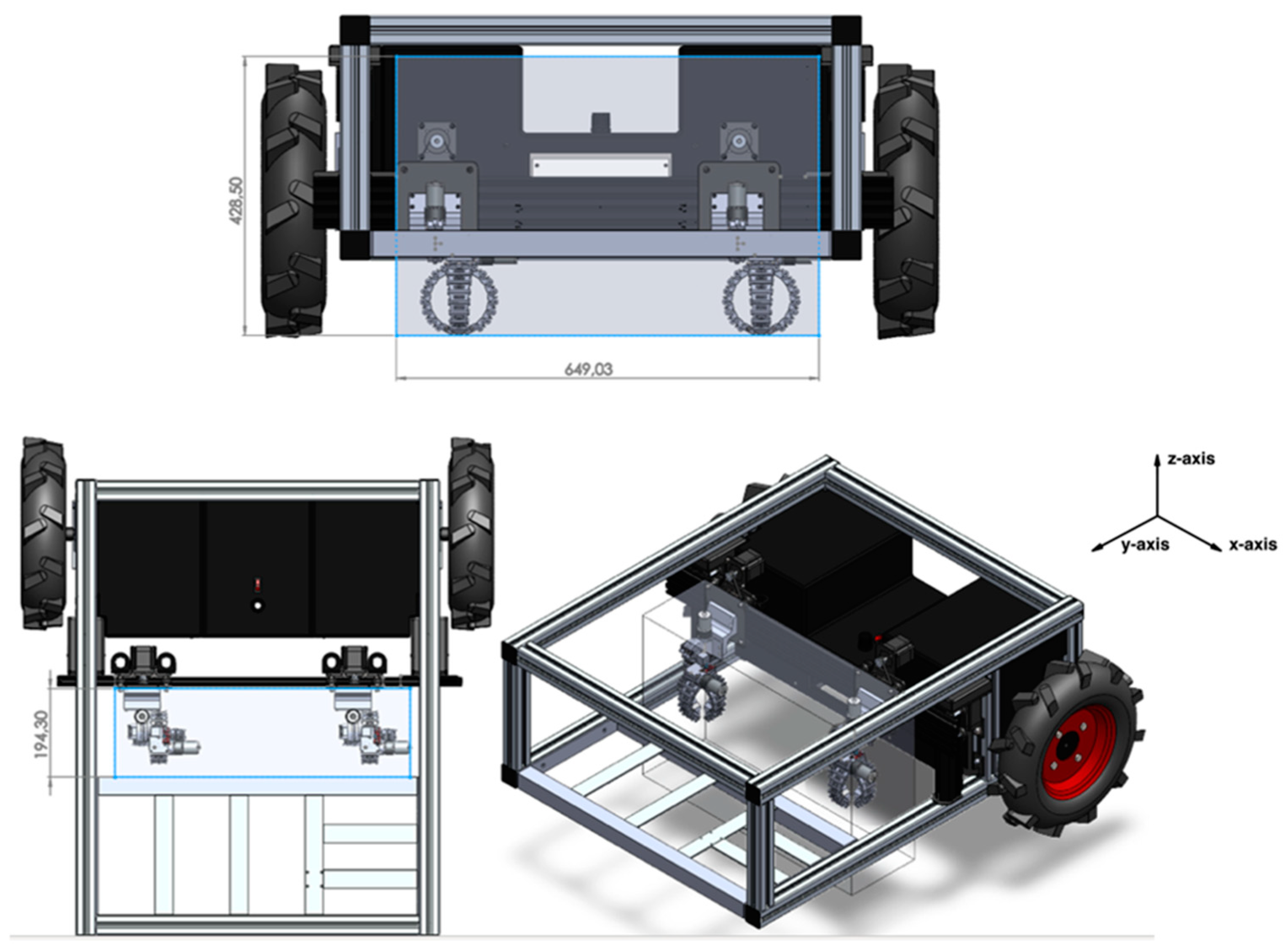
2.1. Robotic Rover

The Robotic Rover for Agricultural Applications (R2A2) proposed by [26] is a multitasking agricultural land robot that aims to autonomously perform herbicide spraying in a particular manner in peach orchards. The robotic system has two functions performed at different times. The first consists of carrying out precision herbicide spraying at the beginning of the year, as this is the time when the weeds are still small. The second, at the end of the crop, will perform the collection of fallen peaches on the floor of the orchard [26]. During the growth of the crop, it is equipped with cameras and artificial intelligence algorithms that, by using image processing, will perform the detection of fruits, to count them and, thus, provide a more assertive forecast of production, and also will perform classification to enable the early identification of fruit diseases and, thus, allow the fruit grower to take the necessary measures in time. With this, the environmental impact tends to be minimized, since the amount of herbicide used in weed control will be reduced because of precision spraying. Moreover, the collection of fallen peaches avoids the proliferation of insects and bacteria that grow on the fallen fruit and will hibernate until next year’s crop. The platform also aims to reduce labor costs associated with manual peach removal activities.
The robotic platform was built to be able to move autonomously in the orchard and perform tasks close to the tree trunks, however, without passing between two of them and moving only in between the rows of trees. The robot was designed to overcome terrain inclinations of up to 20° and to move under covers larger than 600 mm. Table 1 presents values referring to the other specifications of the robot.
The modelling of the prototype was developed with Solidworks CAD software (Dassault Systèmes SE, Vélizy-Villacoublay, France). With this, the planning of the entire construction and assembly of the robot was performed. The tool also possible the extraction of technical drawings possible that helped in the construction of the system, including all drawings of the parts that were manufactured with the aid of computer numerical control (CNC) machines. Figure 1 shows an exploded view of the vehicle performed by the CAD software used.
The structural component of the robot is formed using a 45 × 45 mm T-slot aluminum profile from Boch Rexroth, which creates a very strong and lightweight structure. This solution was selected because it is easy to assemble and it also allows easy attachment of different parts that can be added after the project is completed. In addition to the easy repositioning and adjustability of the structure, the robotic platform has a Cartesian arm for spraying. This robotic arm has 5 axes and directs the spraying nozzle and the gripper that will perform the collection of the peaches that are fallen to the ground. In this case, it will be possible to perform tasks in an extension of 1200 mm, because the driven systems can work outside the robot’s structure to perform activities close to the stem of the crops.
Figure 2 shows the robot’s isometric perspective, that is, the final 3D drawing of the robot platform that is already assembled and with all components that will help it perform its tasks. The 3D model was an asset because it allowed the optimization of construction resources, improvement of components, and restricted possible assembly errors. With this, it was possible to create a more precise bill of materials that helps in the management of the assembly project, avoiding any interruption due to a missing component.
In Figure 3, you can observe the vehicle in operation in the field. The R2A2 ground robot, which was developed and tested, shows promise in several crop stages such as in decision support for the producer.
A Cartesian robotic manipulator was incorporated into this robot for fruit collection and spraying in agricultural fields. The robotic manipulator is intended to be an integral part of the agricultural environment in the fight against food waste and the reduction in pests and diseases. Activities such as the collection of fallen fruit in orchards, which require human resources and involve a cost, can be used to direct these fruits to animal feed or organic fertilizers and enhance the reduction in microorganisms that can result in diseases and pests. Currently, about 40% of food loss is caused by pests, pathogens, and weeds [27,28]. Based on the technical specifications of the platform, it is possible to obtain the working envelope of the Cartesian axis and, consequently, the maximum dimensions of the robotic gripper developed by Tavares [29]. Thus, using the resources available in the SolidWorks software, the work envelope was determined: Δx = 649.03 mm, Δy = 194.30 mm and Δz = 428.50 mm. Figure 4 shows the work envelope in shaded gray, as well as its dimensions.
A robotic gripper is incorporated to the robotic manipulator for the task of picking fallen fruits, for which its construction of the final prototype was divided fundamentally into three strands: construction of the mechanical system, electrical system, and programming of the control system. In the end, both systems interconnect with each other. To conclude the mechanical construction of the prototype, the rotation system is coupled to the spacer (1) (see Figure 5 for the numerical markers correspondence) and the spacer is coupled to the front plate of the y-axis; consequently, the gripper (3) is coupled to the rotation system (2). An isometric view of the developed robotic gripper is shown in Figure 5. Before starting the field tests of the developed technological solution, simulations were performed to speed up the algorithm development process.

2.2. CoppeliaSim Simulator

After a study performed, the CoppeliaSim simulator (Coppelia Robotics AG, Zurich, Switzerland) was chosen [30] since this tool has several features such as physics engines, a comprehensive model library, the ability to interact with the environment during the simulation, and most importantly the manipulation and optimization of meshes. This software can be used for the development of rapid prototypes, simulation of automation systems, and teaching. The program has a large collection of existing robots and sensors on the market and can import new models or create them using integrated modeling capabilities. If the Robot Operating System (ROS) is used, it is even possible to connect it to existing robots [31]. This simulator also allows the control of robots through six types of programming, all of which are mutually compatible in the simulation. This possibility is due to CoppeliaSim’s application programming interface, which allows the integration of ROS and BlueZero topics, the creation of APIs for remote clients, plugins, and other forms of programming. Since CoppeliaSim allows testing programs created on different platforms, it is a very versatile solution. It also has four physics engines and allows collision detection, distance calculation, simulation with proximity sensors, and vision systems. For all these functionalities, the software is often called a “Swiss Army knife” in the robotic simulation community [3,32].

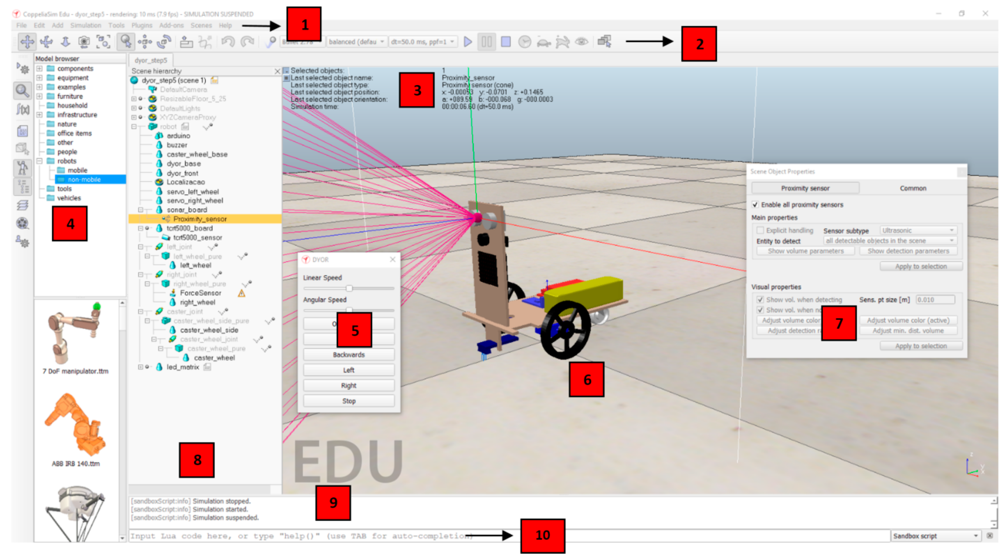
2.2.1. CoppeliaSim’s Graphical Interface

Figure 6 shows the application window where you can view, edit, interact, and simulate the “scene” and its respective models. In addition to this, there is also a console window, which is a non-interactive element that only allows you to show information about the simulation (e.g., plugins that were loaded and the state of their initialization), which for the work in question is not relevant since there was no interaction between external software or machines such as robots and CoppeliaSim.
In the CoppeliaSim graphical interface, there are several elements specified as follows (the correspondence with Figure 6 is performed by using numerical markers):
  • Menu bar (1): Allows access to the simulator features that, unlike the most commonly used ones, cannot be accessed through interaction with models, pop-up menus, and toolbars;
  • Toolbars (2): These elements are present for the user’s convenience and represent the most used and essential functions for interaction with the simulator, specifications);
  • Informative Text (3): Contains information allusive to the object that is selected at a given moment and of parameters and simulation states;
  • Model Browser (4): In a top part, it shows CoppeliaSim model folders; on the other hand, in the bottom part, there are thumbnails of the models that can be included in the scene through the drag-and-drop action supported by the simulator;
  • Dialog Boxes (5): Feature that appears during interaction with the main window and, through which, it becomes possible to edit various parameters relating to the models or the scene;
  • Scene (6): Demonstrates the graphic part of the simulation, that is, the final result of what was created and programmed;
  • Customized User Interface (7): It is possible to make a quick configuration of all the components inserted in the “scene” through this window that appears for each of the objects whenever requested;
  • Scene Hierarchy (8): Here, the entire content of a scene can be analyzed, that is, all the objects that compose it. Once each object is built hierarchically, this constitution is represented by the tree of its hierarchy, in which by double-clicking on the name of each object the user can access the “Custom Interface” that allows it to be changed. It is also with this simulator functionality, through drag-and-drop, that the parental relationships between objects are created (child objects are dragged into the structure of the parent object);
  • Status Bar (9): The element responsible for displaying information about operations, commands, and error messages. In addition, the user can also use it to print strings from a script;
  • Command Line (10): It is used to enter and execute the Lua code.

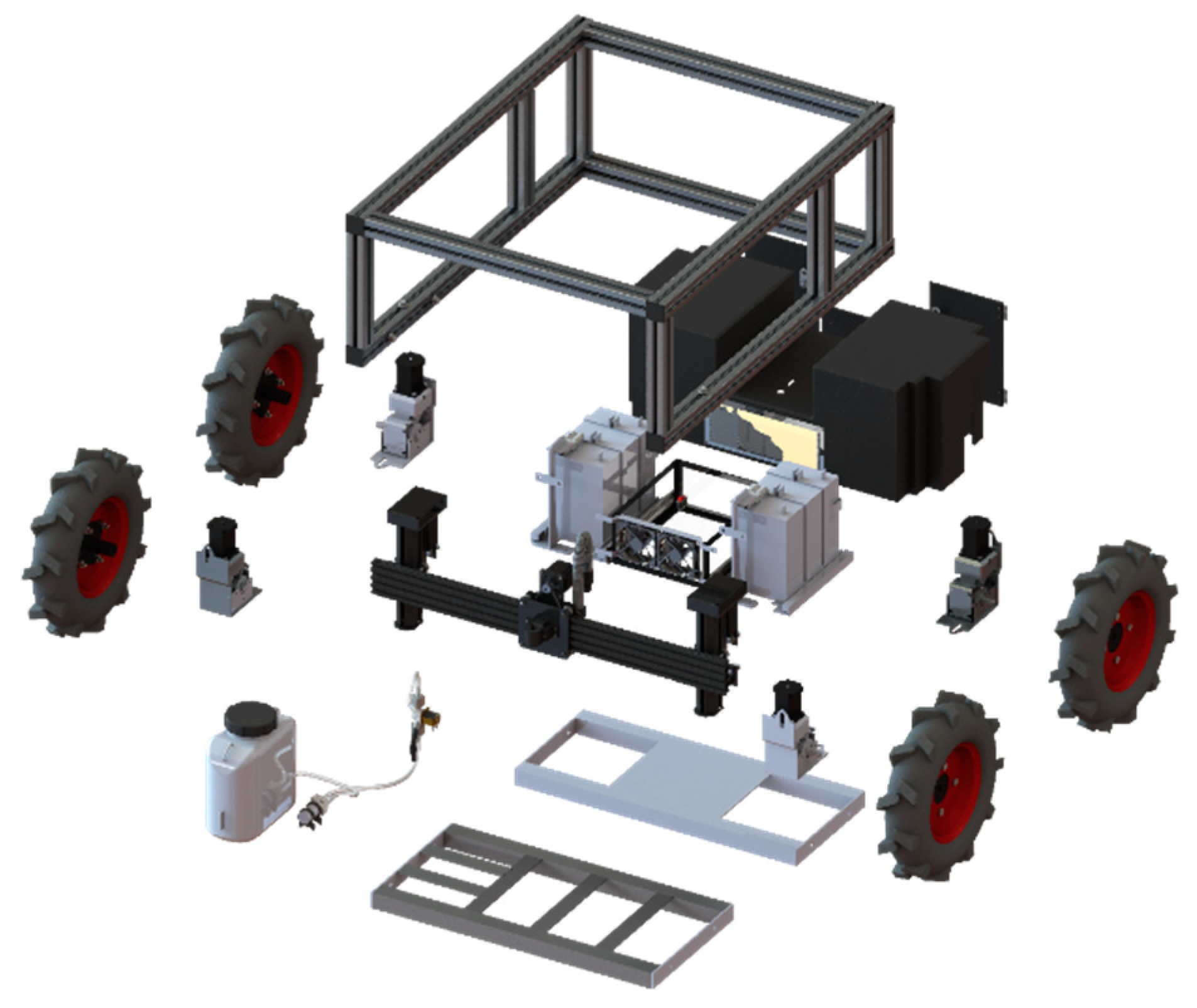
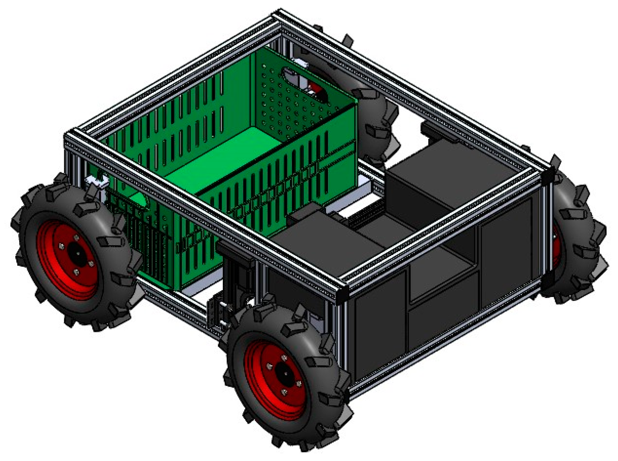
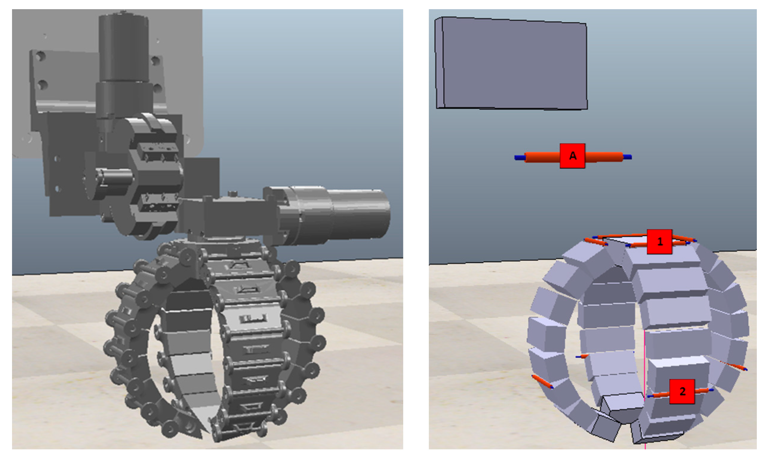
2.2.2. Robotic Platform Creation

The components (chassis, wheels, shafts, accessories, and gripper) were imported into the simulation. After this import was performed, primitive shapes were created with dimensions and physical properties (e.g., density, weight, friction, damping, etc.) identical to those of the original components to make the behaviors of the robotic platform as similar as possible to reality. It should also be noted that when importing the various components of the robotic platform to the simulator, some objects that were negligible for simulation purposes and that only made it more difficult, such as screws and fixtures, were ignored.
Once this step was concluded, we were left with the original design (shapes made of triangular meshes) and the primitive shapes that will be used for simulation purposes, both of which can be observed in Figure 7.
The main work that is intended to be performed is the fruit harvesting, and the mechanical gripper was already installed on the x-axis support. This gripper was a work also developed by the PrunusBot Operational Group, and it is intended to be used in the robotic platform for fruit picking [29]. This mechanical gripper is represented in Figure 8, which shows the design imported from the original file, in convex shapes, and also the primitive shapes with the respective joints to be used, which were created from that original design and will serve as the basis for the simulation. The gripper is operated by the main joint (A), which enables a lifting motion by rotating 90° under this joint. To operate each finger of the gripper, two joints represented with markers (1) and (2) in Figure 8 were used.

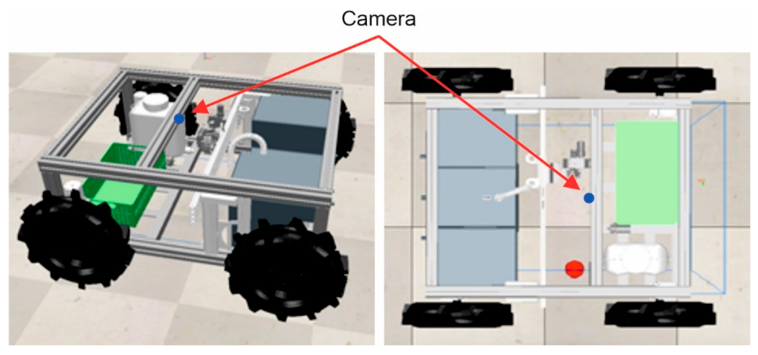
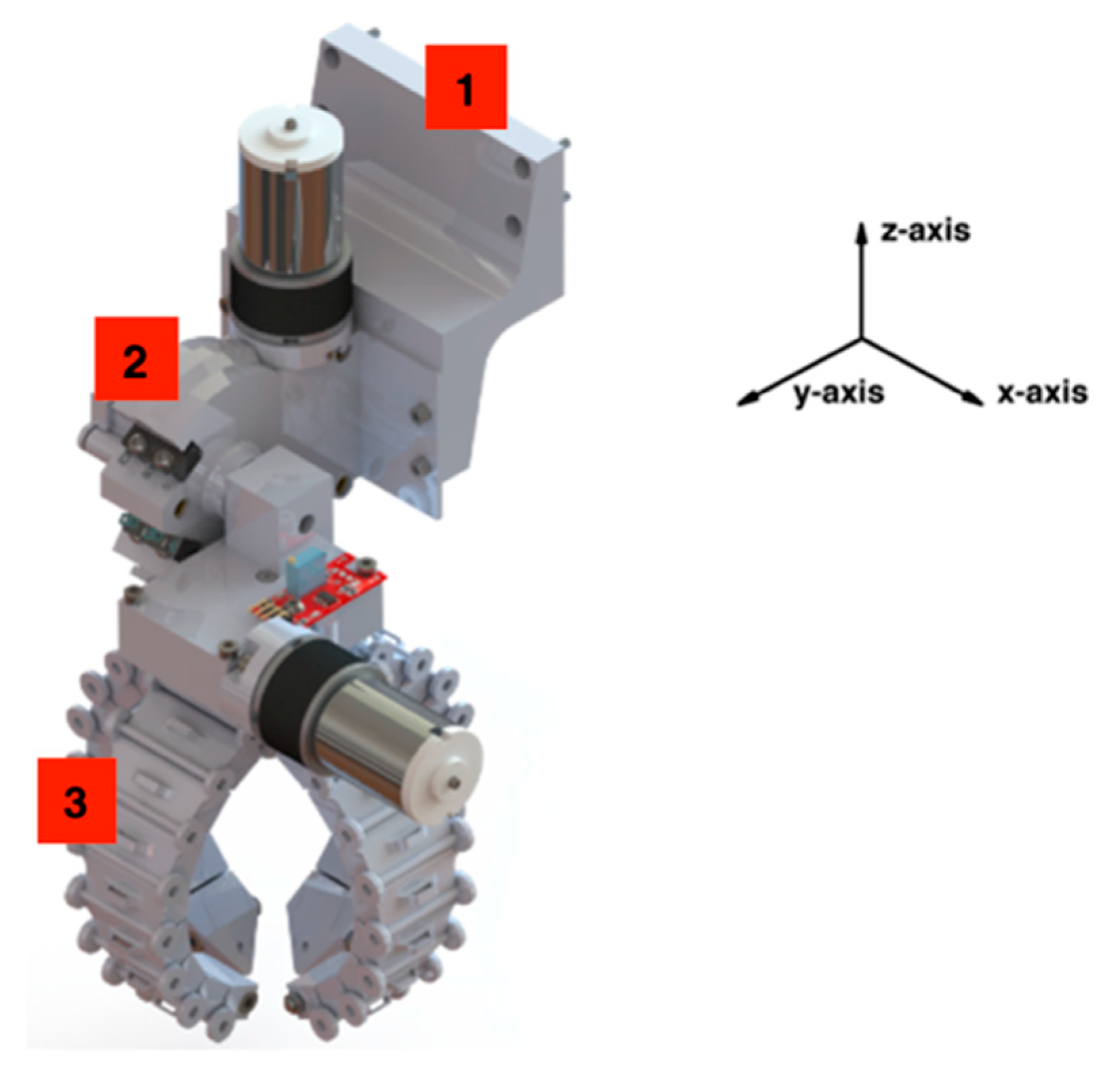
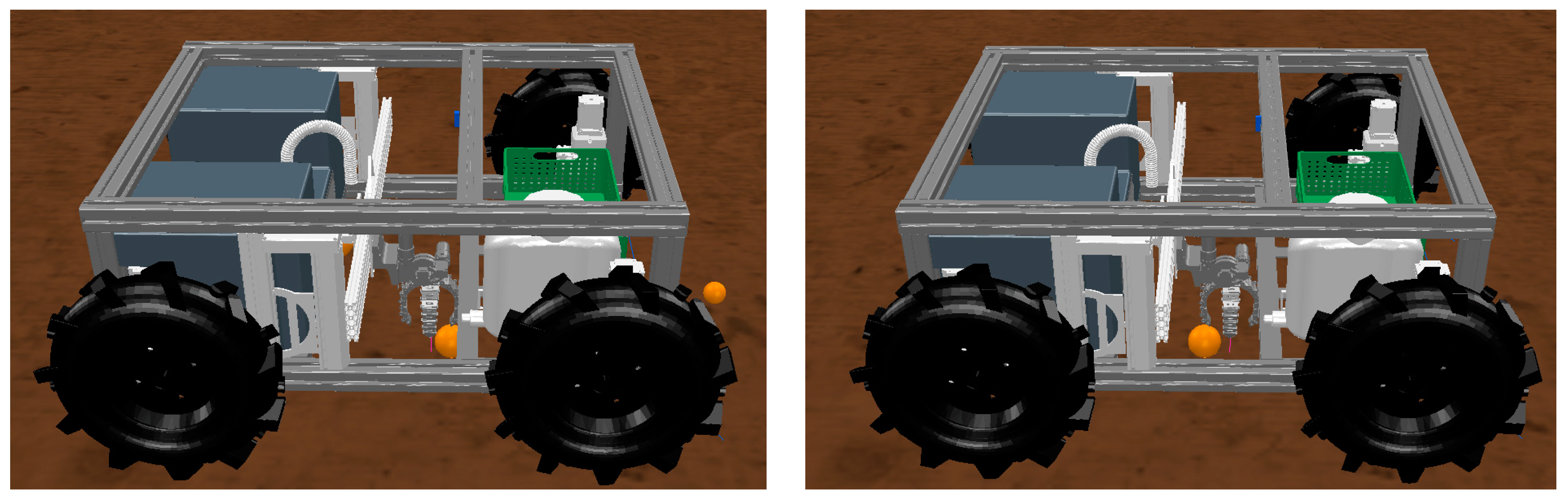
2.2.3. Inserting a Video Camera

Once the robotic platform was created, a video camera was added for capturing images, thus being able to locate the objects to be captured. The camera used in this robotic platform is the “Raspberry Pi Camera v2”. This camera allows the capture of images in three different resolutions: 1080p30, 720p60, and 640 × 480p90.
CoppeliaSim allows the insertion of various types of sensors, including vision sensors. After the camera was inserted and positioned identically to the one installed on the robotic platform, it was only necessary to configure various parameters.
The camera was installed in an identical location to the original prototype to ensure that the viewing angle will be the same as in reality. The camera was installed on top of the robotic platform, and an aluminum profile was added in the middle of the platform’s structure to allow a view of the central and lower part of the platform. Figure 9 highlights the position of the camera represented by a blue dot.
With the camera properly installed and configured, the next step was to define the areas of the image that should be analyzed when it is in operation. The definition of these zones can be observed in Figure 10.

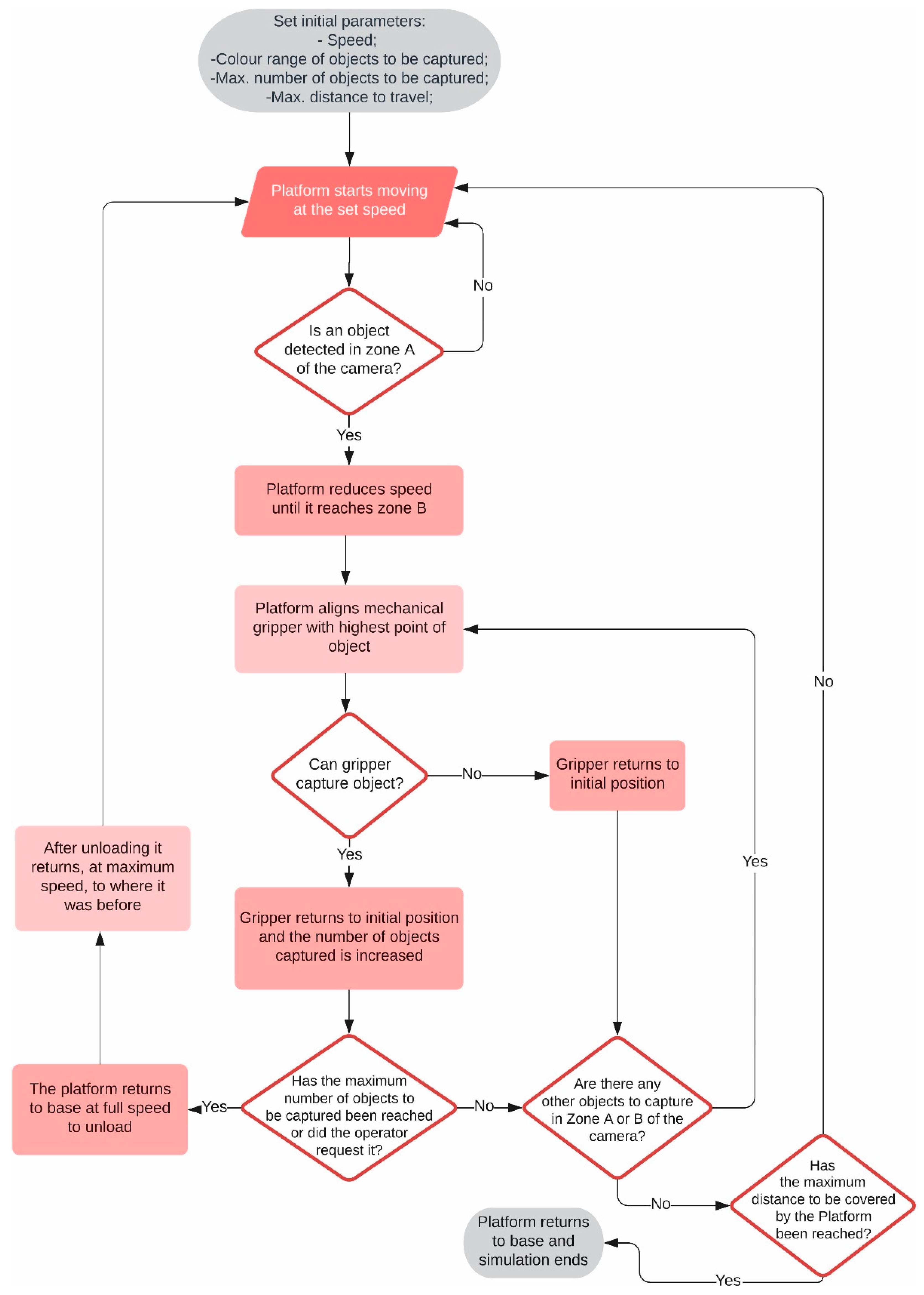
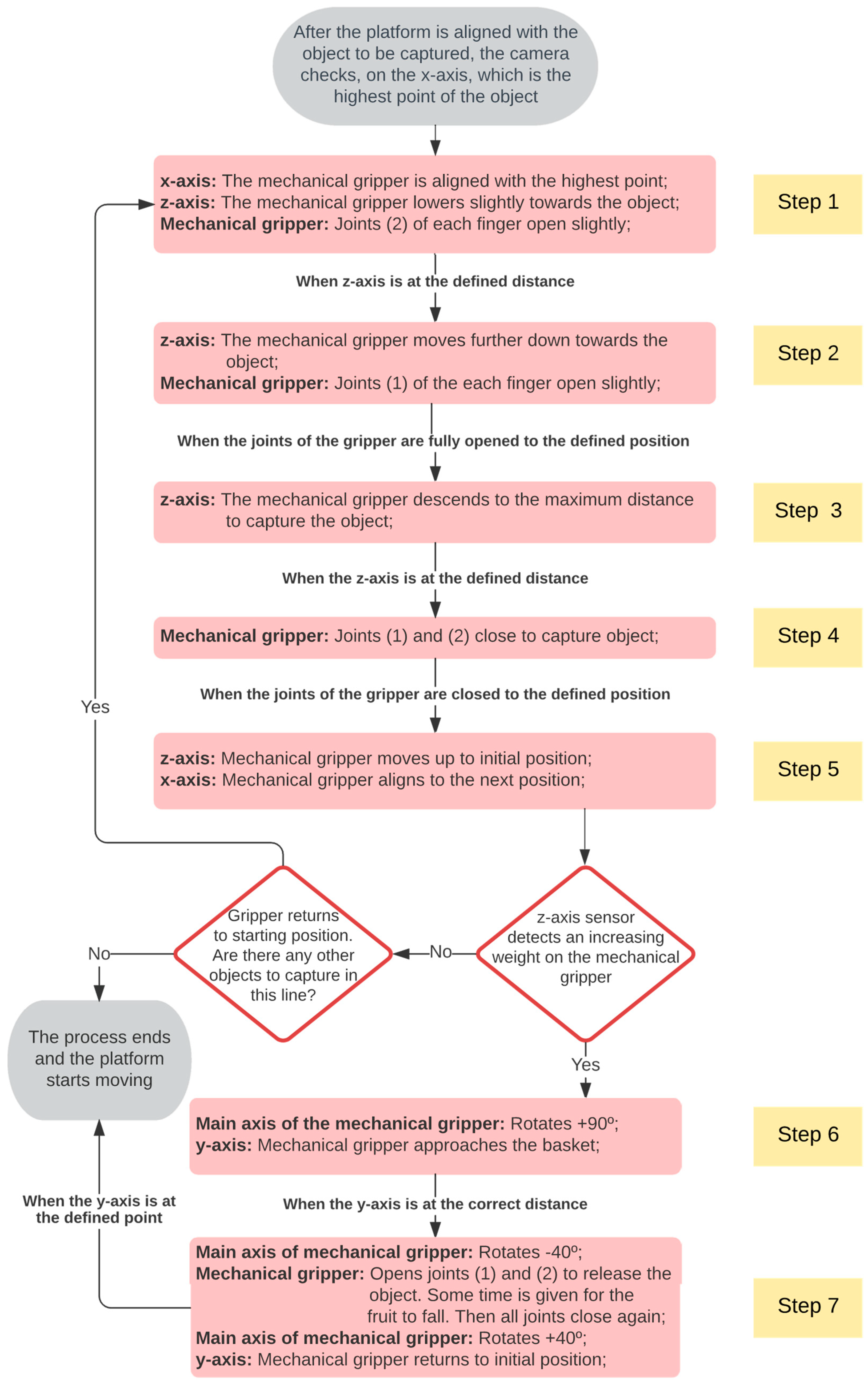
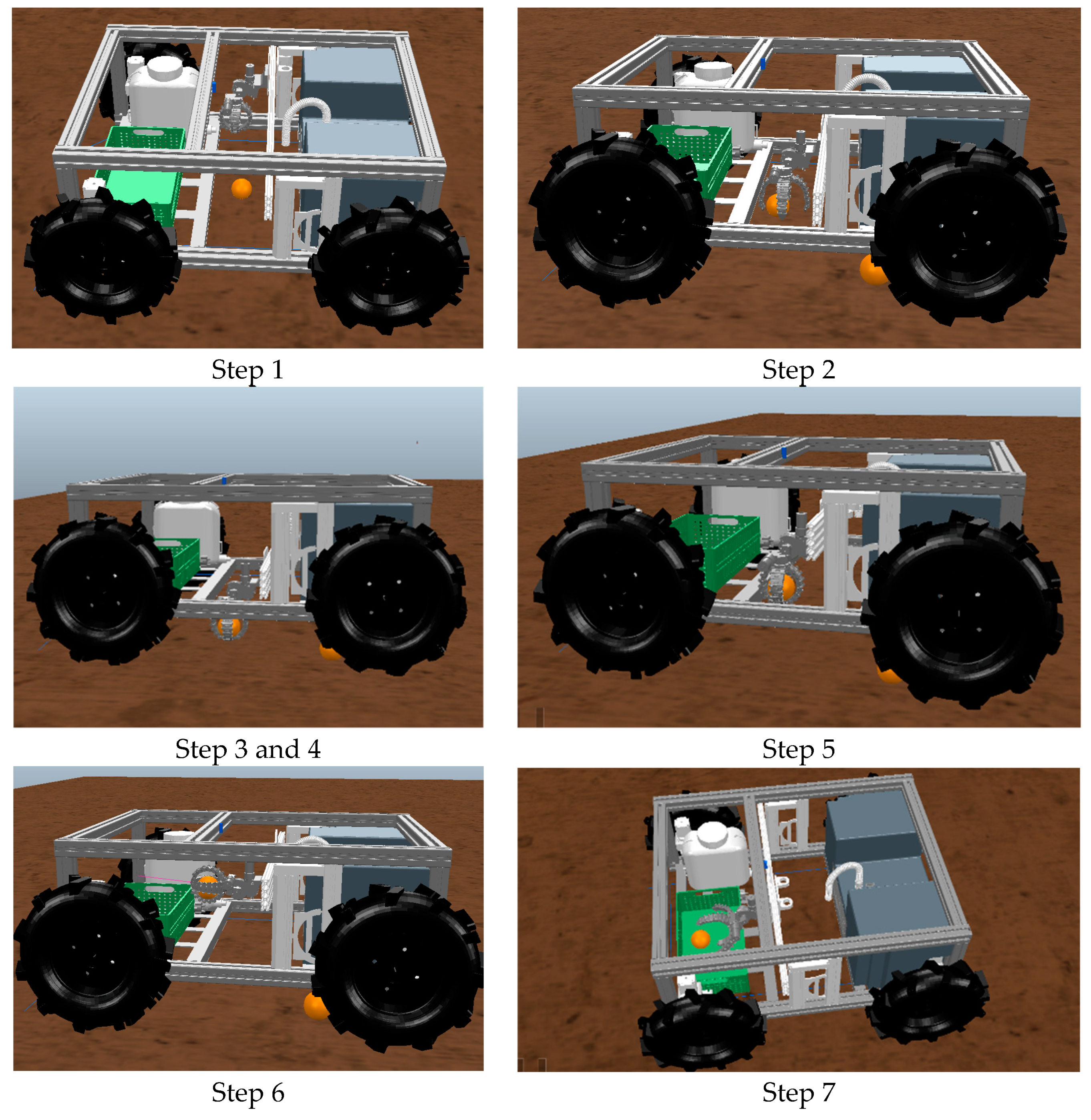
2.3. Proposed Algorithm

The purpose of this robotic platform is to detect and collect specific objects, in this case fruit, which will be scattered randomly on the floor of an agricultural field or in an area to be defined. However, to create an algorithm that fulfills this function, there are other factors to take into account and even external factors that must be observed for the robot’s mission to be successful. Thus, in an initial phase, the various steps and logical conditions that this algorithm will have to fulfill are idealized. This idealization process was performed through the flowchart presented in Figure 11. This flowchart presents all tasks performed by the robotic platform software to operate in the field with the desired objective of capturing objects.
For object (fruit) collection, a set of movements that will need to be made by the platform for object capture has been defined. These movements are described in the flowchart in Figure 12. The movements required for object picking were divided into 7 steps. The flowchart describes, for each step, all the associated movements in terms of the x-y-z-axis and the gripper and the condition required to proceed to the next step.

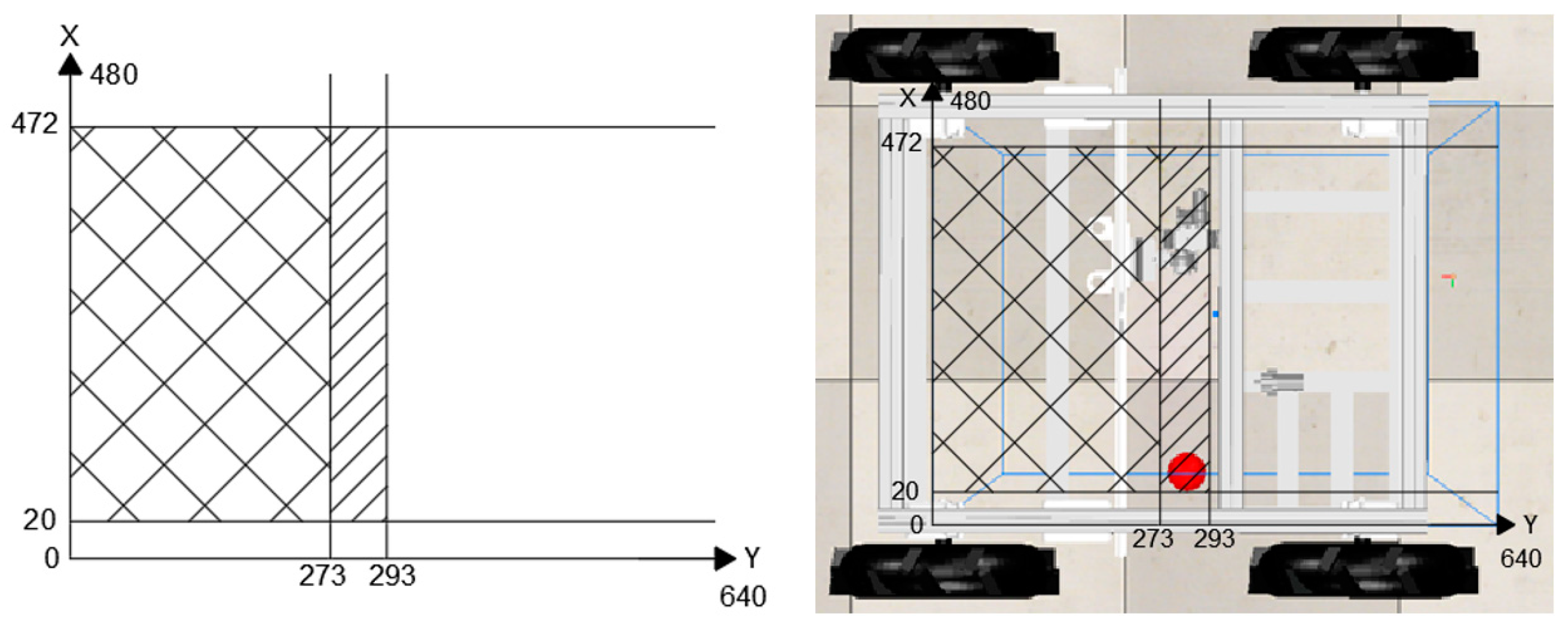
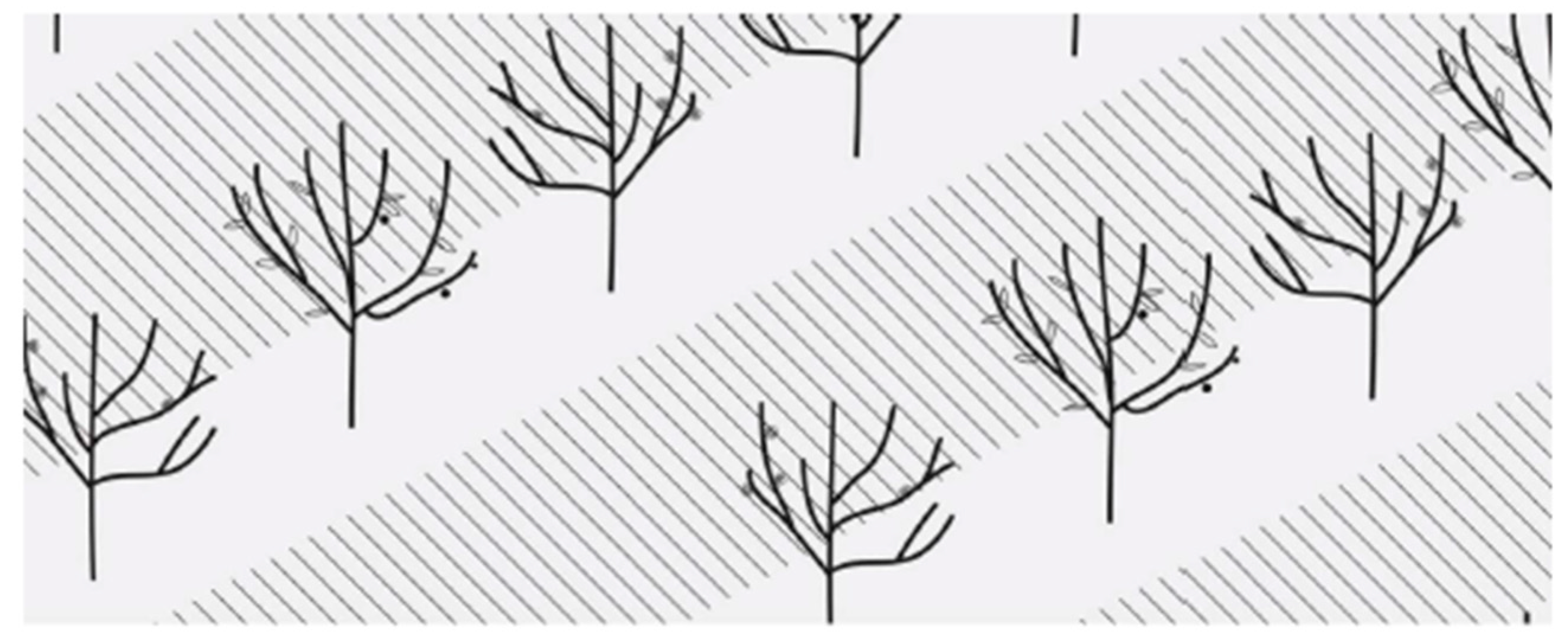
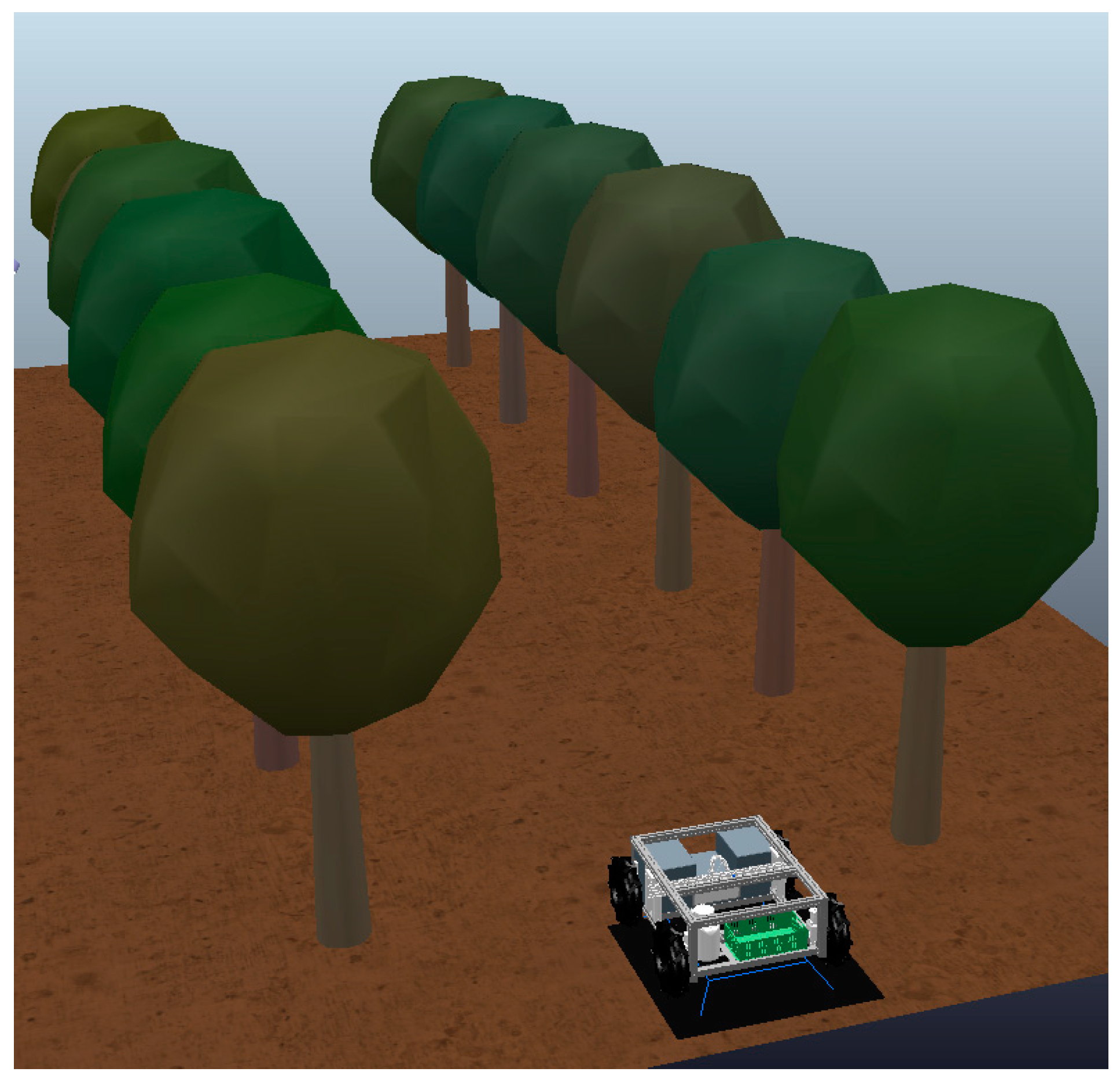
2.4. Recreating a 3D Orchard Environment

Having recreated a robotic platform identical to the one existing in the CoppeliaSim software and also an algorithm to control the platform, an environment similar to the crop fields is now created in which the platform will operate. As already mentioned, this platform was designed for use in peach orchards, namely in the orchards of the Beira Interior region, since this region alone represents about 49.2% of national production [33].
Given this fact, the 3D model to be recreated should be similar to the orchards of this area. According to Simões [34], the most frequent measurements in peach orchards in Beira Interior are 5 m × 2.5 m, 5 m × 3 m, 4.5 m × 2.5 m, and 4.5 m × 2.75 m. The first measure is related to the distance that should exist between each plant and the second refers to the distance between the rows that the furrow forms, the inter-row, as observed in Figure 13.
For the creation of the 3D model, a compass of 4.5 m × 2.5 m was used because it was found to be the “worst-case scenario” in the sense that the interline is the smallest width and has trees closer to each other. Next, the texture to be applied in the simulation use plan was selected, and a texture of dark brown tones and relief designs was selected but without any inclinations. The final model can be observed in Figure 14.
Since peaches can have various sizes, placing objects of also various calibers and weights in the simulation model was decided, and this included objects with diameters between 50 and 90 mm and weights between 100 and 150 g, with the largest weight being assigned to the largest objects, as observed in Figure 15. All these objects were inserted as primitive type shapes with spherical geometry. Regarding color assignation with respect to these objects, orange tones were used, since it is the approximate color of peaches. However, several shades of orange were used to test the ability of the algorithm.

3. Results Analysis and Discussion

This section analyzes and discusses the behavior of the robotic rover when performing the two types of jobs that are proposed. Subsequently, a set of three tests is presented for each of these jobs in which the robotic rover will act. These tests serve to evaluate the algorithm’s ability to detect objects with different parameters and to capture or spray them, depending on the operation to be performed. Finally, a brief analysis will be made on the results that were obtained.

3.1. Rover Behavior

3.1.1. Operating Speed

When starting these simulations, it was already known that it would be a somewhat lengthy process since the operating speed was low, and the size of the agricultural areas was large. Initially, and to try to improve this aspect, we tried to use higher operating speeds. However, it quickly became apparent that conducting this would place the detection of objects at risk since the camera’s vision time was shorter. Thus, the main conclusion drawn was that the operating speed should never be higher than 0.63 m/s. For the values referred to in scientific literature and those already mentioned above, these are quite high speeds.
In addition this issue, it is also important to mention that the alignment of the tool in use with the object was often misadjusted in the sense that the robotic rover would always be slightly ahead of the object, and this situation is represented in Figure 16. As observed, it would always be more serious when the task in progress was capturing objects because, in this process, it is important to have a good alignment of the mechanical gripper with the object to be captured.
Initially, there was an attempt to correct this point by adding a condition to the algorithm that, whenever this happened, the robotic rover would move backward until it was in perfect alignment. However, it was found that the time lost in this process was identical to operating the robotic rover at a lower operating speed.
For all these reasons, the strategy of viewing the camera were with the two zones chosen. In this manner, it was possible to optimize the operating speeds of the robotic rover by using two speeds. In the object detection phase, the robotic rover moves at an “average” speed of 0.63 m/s, which is enough to detect objects, and as soon as they are detected, the robotic rover starts moving at a “minimum” speed of 0.42 m/s, thus managing to perform a better analysis of the detected object and also ensuring the speed slowdown required for the robotic rover to be aligned with the object to be captured or sprayed.

3.1.2. Image Processing

As already mentioned, the vision sensor that is in the original robotic rover allows various resolutions. Moreover, to improve the fluidity of the simulation, the lowest resolution of the vision sensor was used. However, from what can be found in CoppeliaSim user forums and other platforms, this resolution is still too high. For this simulator, lower resolutions were normally used, and this can create some delay. Coupled with this issue is also the code created because if it performs many cycles of code over the vision sensor, it renders the simulation even more complex. This is also why we tried to maximize the code to be applied to image processing in order to improve the fluidity of the simulation.

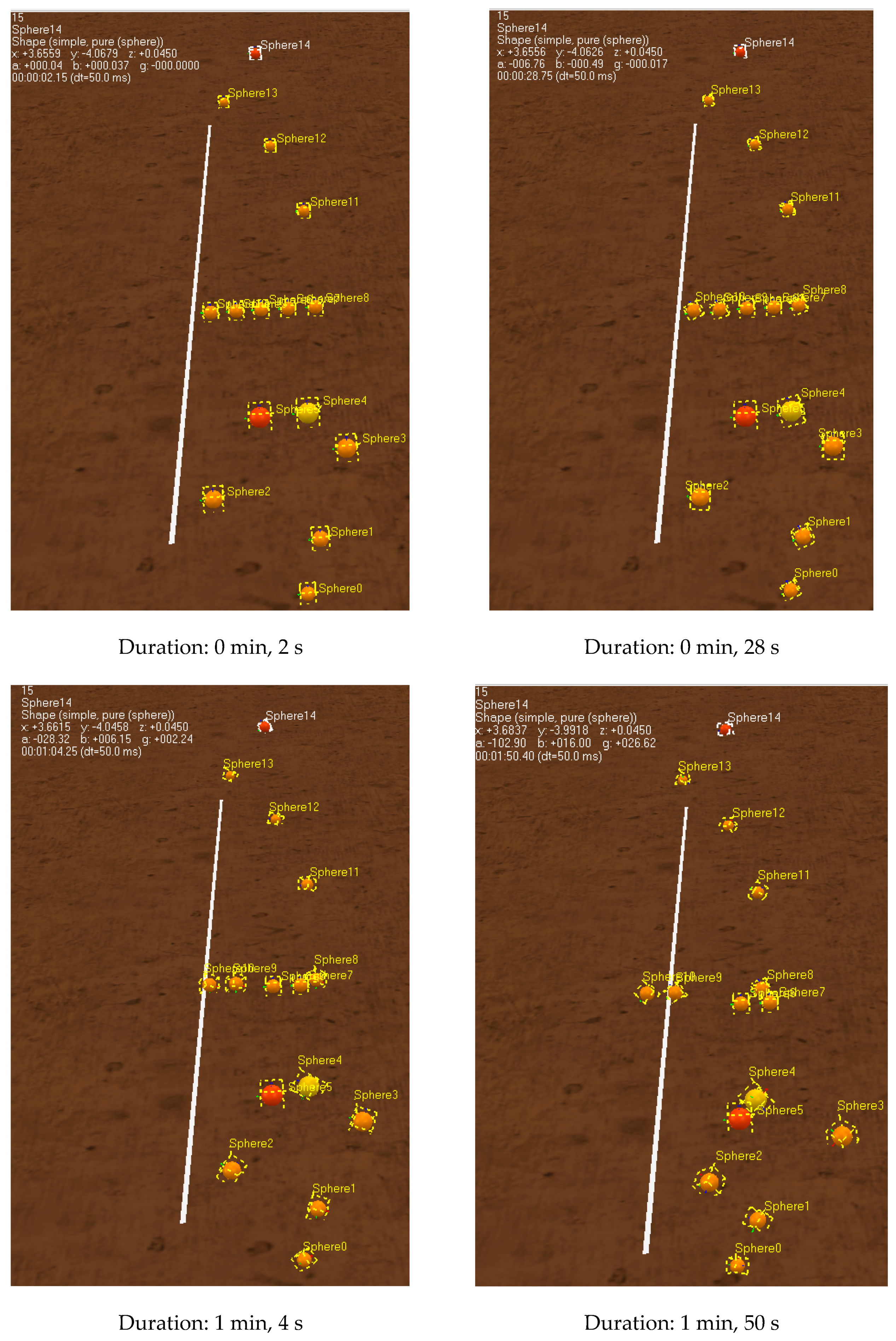
3.1.3. Operation Time

In addition to the points mentioned above that can make the simulation more time consuming, there is also the issue that, when the task to be performed is capturing objects, the operation time will be even longer, for it was verified that the time to capture the object was also somewhat time-consuming in the sense that it was necessary to perform several maneuvers demonstrated in Figure 17.
According to Figure 17, it can be observed that, in step 1, the robotic rover aligns with the object, and the mechanical gripper runs in the x-axis until it is also aligned with the object. In step 2, the z-axis prism lowers the mechanical gripper, and the gripper clamps are opened. In steps 3 and 4, the gripper reaches the object and closes to capture it. In step 5, the z-axis moves the mechanical gripper back up to the initial position. In step 6, the mechanical gripper will rotate 90° and the y-axis prism will send the mechanical gripper forward toward the fruit package. In step 7, we can already observe the object being poured into the package; posteriorly, the mechanical gripper and all prisms return to the initial position.
To maximize the operation time in performing all these maneuvers, we tried to apply some techniques such as improving the algorithm itself, which is when each of the functions is activated. We also tried to increase the operating speed of the prisms or even changing the parameters in the Proportional-Integral-Derivative (PID) control, which the software already has for when the joints are placed in the position control mode.
However, the improvements achieved were minimal, and it should also be noted that, in the case of changing the operating speeds, the PID control of the prismatic axes is somewhat ambiguous, because there is no point in inputting a very high value if the prisms of the original robotic rover cannot operate in these characteristics.

3.1.4. Physical Simulation Engine

As mentioned, CoppeliaSim has four dynamic simulation modules that serve to calculate, in a realistic manner, the interactions that may occur between rigid bodies. In the several simulations performed, all four modules were tested because, according to Miranda [31], these modules work mainly by approximations, and it is interesting to use more than one to confirm the results.
From the several simulations performed, it was observed that the results obtained for the different simulation modules were similar, except for the Bullet 2.78 module, because when it was used for the object capture operation, it was observed that, when starting the simulation, the objects to be captured, which are spherical and the usage plane is completely flat, automatically started to rotate through the field while eventually disappearing. This problem is represented in Figure 18 in which it is possible to verify that, in the first 30 s, the objects do not move much; however, from then on, the objects started to gain some acceleration, and after 1 min, the differences are already noticeable. From then on, the differences tend to be greater and greater since the acceleration of the objects is constantly increasing.
It is interesting to observe that the objects have a tendency, in most cases, to roll over to the left side of the scene, as shown by the line placed on the ground. It was also verified if the used plane had any inclinations, which was not the case. This was the case even though the friction parameters of the objects and the use plane were set to maximum values. As such, this module was disregarded for the object capture operation because it was understood that it did not correspond to the reality of the simulation.
Another aspect that was verified in several simulations performed in which the physics engines available in the simulator were switched is that the object detection process was performed successfully; however, for the object capture operation, it was usually necessary to change the parameters of the mechanical gripper joints and the prism axes in order for the capture to be performed successfully. However, since the physical engines simulate approximations with respect to reality, it is normal that some differences arise, especially when such a meticulous and specific step is being performed. Moreover, Armesto [35] mention this condition and even suggested the use of a “fake pick up” to overcome this problem. Thus, it is deemed as irrelevant in this aspect because the important thing is that, if this simulation is replicated with respect to reality, these parameters are adjusted to the reality of the different engines and prisms.
Once the analysis of the various dynamic simulation modules available in the software was concluded, the Newton Dynamics module was used because it was considered to be the module that best represented the reality of a crop field and the behavior of the robotic rover.

3.1.5. Differentiation of Colors in Image Pixels

As mentioned, object detection was only performed in some areas of the image, and one of the parameters used was to check the color gamut that was being read in certain pixels.
The color gamut used in CoppeliaSim is the RGB system, which is an additive color system in which Red, Green, and Blue are combined in various ways to reproduce a wide chromatic spectrum. This system consists of a set of three color codes, each of which corresponds to the amount of red, green, and blue that color has [36].
As a rule, the most usual range of colors proceeds from 0 to 255, where 0 is completely dark and 255 is completely intense. However, CoppeliaSim works with a color gamut from 0 to 1, which is the same principle as the 0 to 255 gamut.
Thus, to perform object detection, it was necessary to analyze the color range of the objects to be used in each of the tasks, and the values measured by the vision sensor for each of these objects are described in Table 2.
For this case, the task to be performed is the capture of objects. It is noticeable, at first analysis, that there is a big difference in the red color code between the usage plan and the various shades of the objects to be captured, and there are also some differences in the green and blue code. However, for the algorithm created, the conditions that were set to be given the “True” condition is that there is an average value in the pixels of the partial image to be analyzed with a red code higher than 0.8 and a blue code lower than 0.2. These conditions were considered because, for the various shades that the peach may have, the red color code will always have a high value and the blue color code only ensures that no object that is too light is captured because the white color has a color range close to the value of 1 in the three codes.
For the case of the weed spraying task, the main differences that are observed include the lower value of the red color code and the higher value of the green color code. Thus, to be given the “true” condition, the requirements to be met are red codes lower than 0.24, green codes higher than 0.32, and blue codes lower than 0.34.

3.1.6. Size of the Objects to Be Captured

Performing object detection by considering only the color range is not very selective in the sense that there is the possibility of an object with the same color range appearing, and this possibility is even greater when operating in an unstructured environment, where controlling the various variables that may arise is not possible. Thus, for the case of the object capture task, another condition was added in which whenever the partial image being analyzed meets the pre-selected color range, this image will also have to be at a certain minimum depth for the logical result to be true.
Note that the average depth value measured by the vision sensor is 0.9 cm in flat terrain without any objects passing through the plane of use, but the more an object passes through the plane of use and the higher this object is, the lower the depth value measured by the sensor. Thus, since the intent of the algorithm is to detect objects of various sizes, the value assigned for this condition to become true is 0.51 cm or lower. This value guarantees that objects with a smaller diameter (which is 0.5 cm) will be detected, and if the object has a larger diameter, the condition will always be guaranteed. It should be noted that, for the case of the weed spraying task, this condition was not included because it was considered difficult to apply in practice since the environment is unstructured and the weeds always have undefined sizes, which is not the case with the task of objects to be captured.

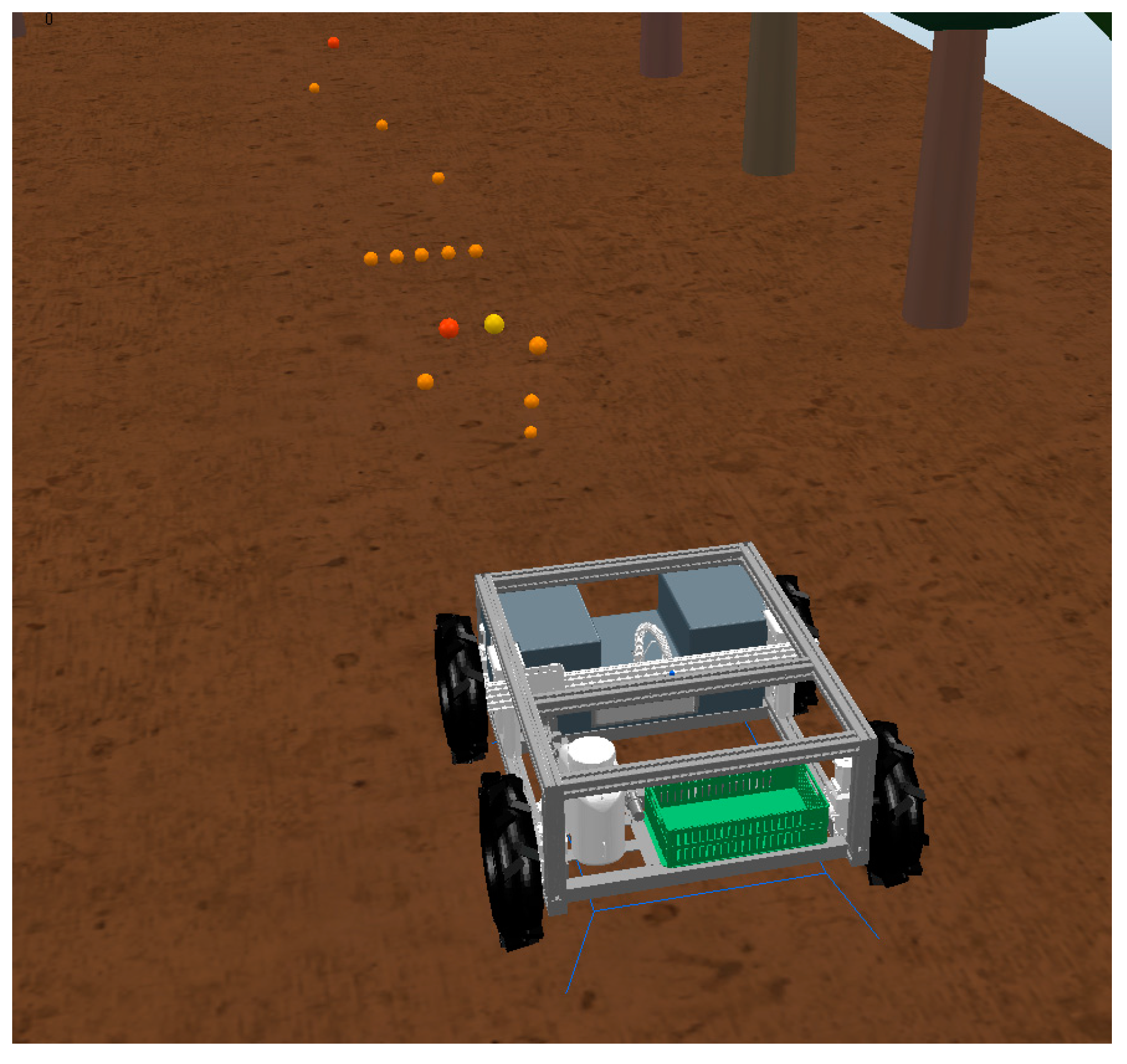
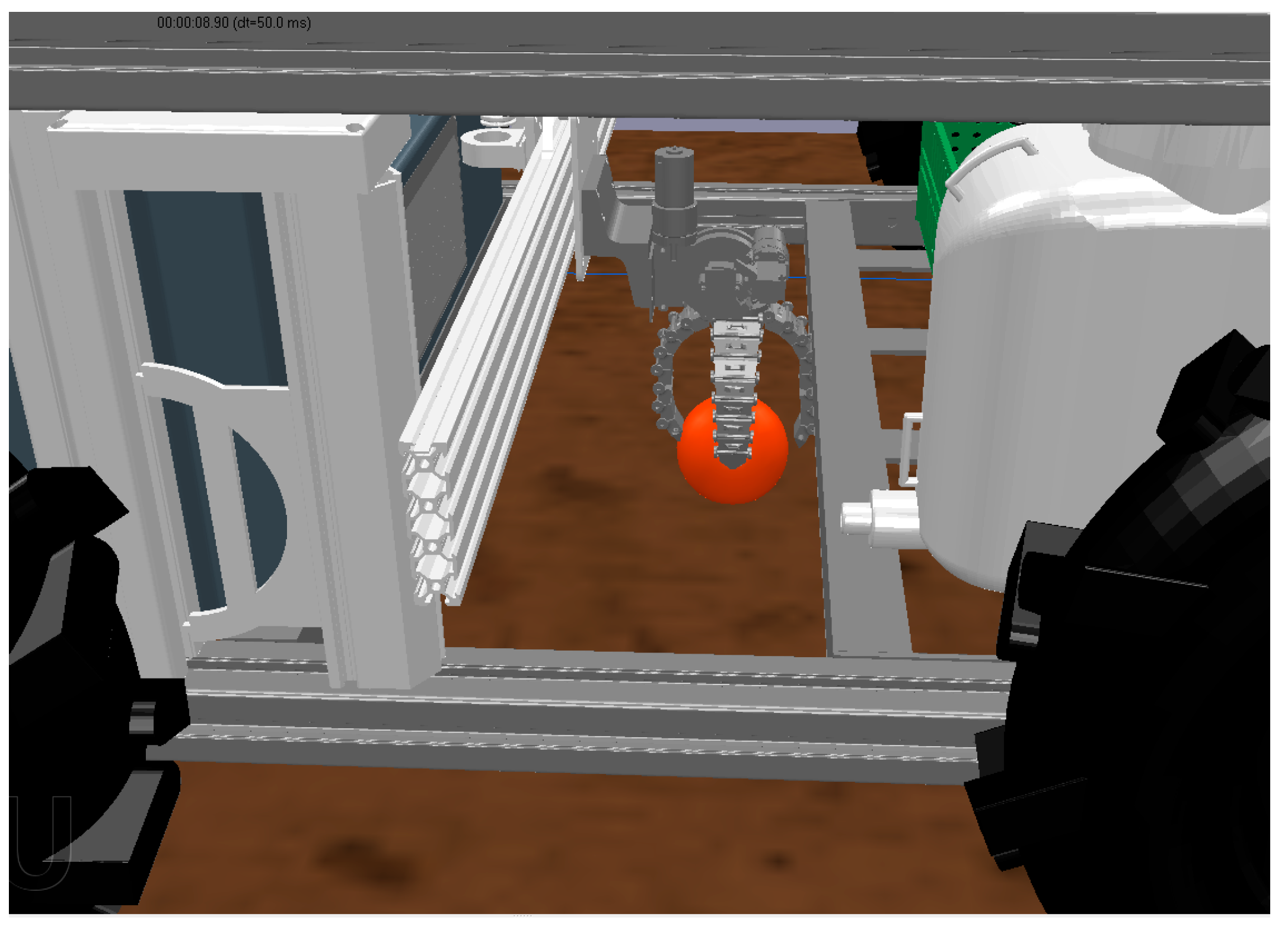
3.2. Case Study Nr. 1—Object Capture

Once all variables in the algorithm, the robotic rover, and the settings of the software itself were defined, a set of tests was performed to evaluate the robustness of the algorithm created. In this first case study, the algorithm’s ability to capture objects was tested. To this end, a set of nine objects to be captured was placed randomly along a 12 m path that the robotic rover will travel on. Additionally, three possible scenarios were defined:
  • Scenario Nr. 1: Objects with equal diameter and with different colors;
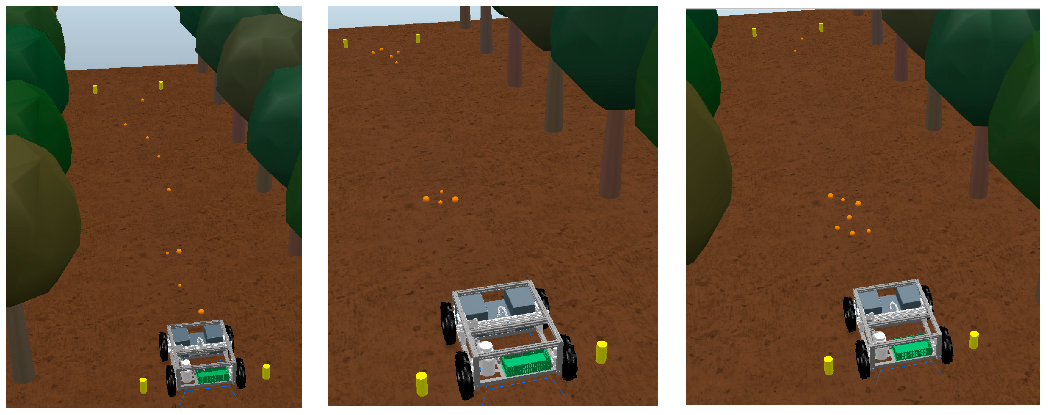
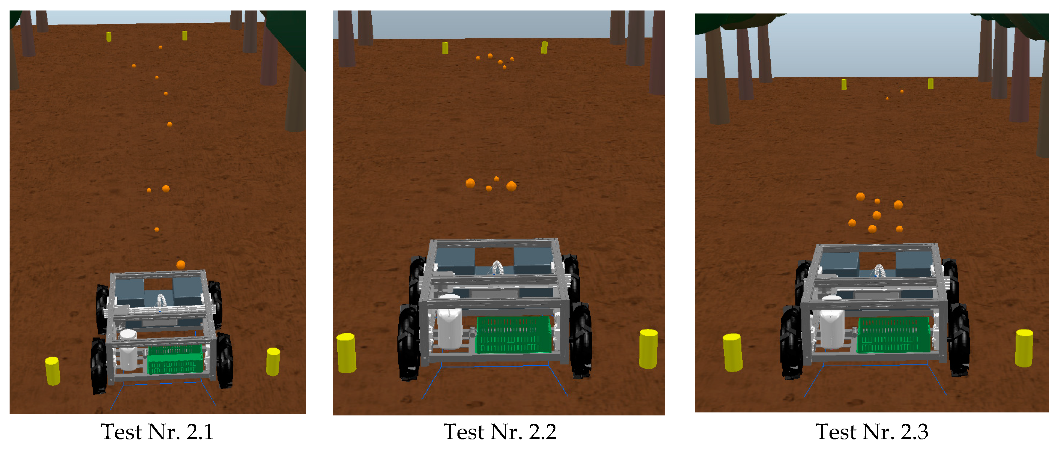
  • Scenario Nr. 2: Objects with various diameters and the same color range;
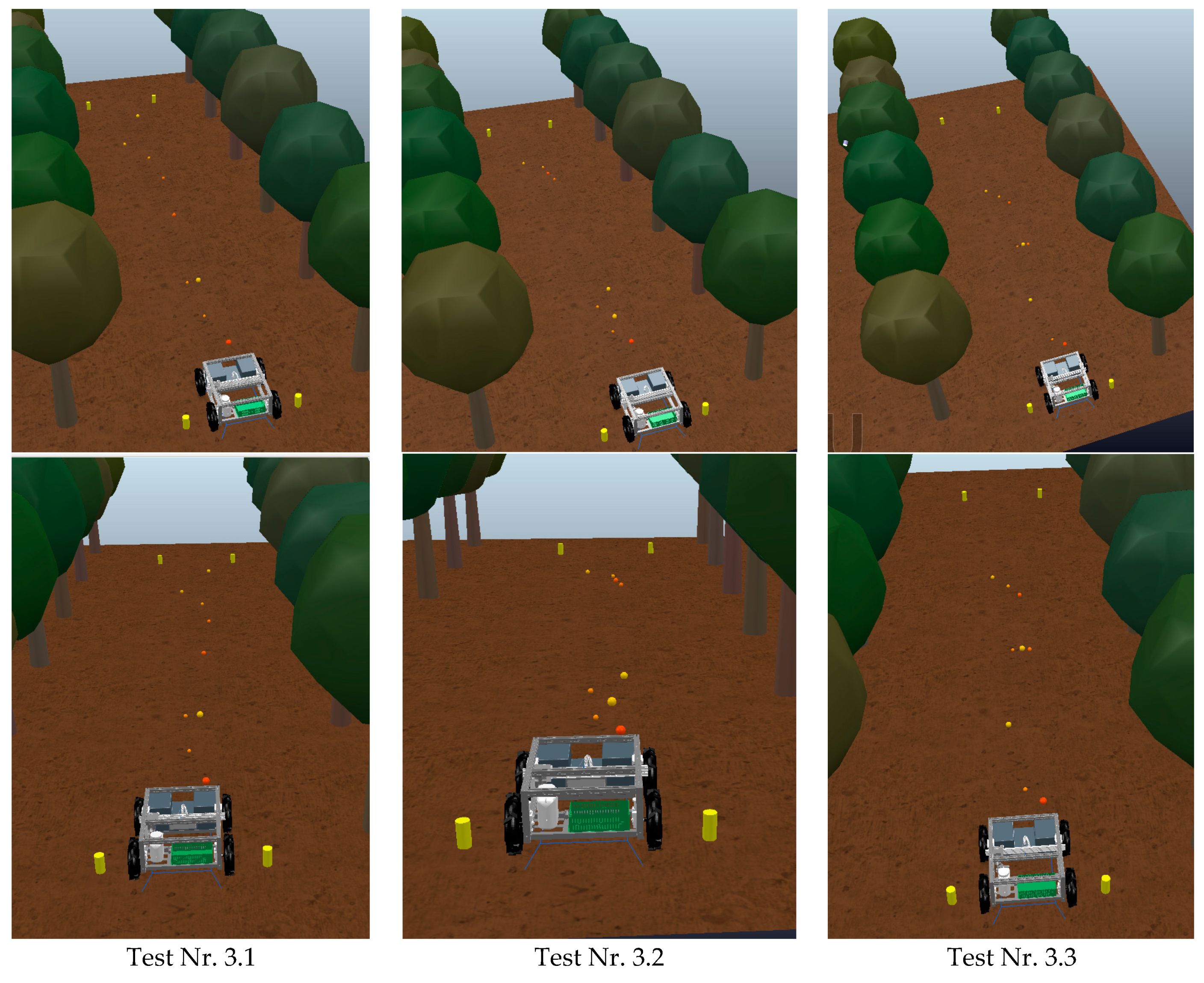
  • Scenario Nr. 3: Different sizes and color ranges.
It should also be noted that, for each of the scenarios, three different tests were performed, in which each of the tests the objects were placed in random positions similarly to the parameter that would be under analysis.

3.2.1. Scenario Nr. 1

In the simulation of this first scenario, the nine objects with a diameter of 70 mm were placed in the use plane. The choice of this size is justified because it is the average value that peaches can have.
The color range used was the one shown in Table 2, and the positions that were given to the objects for each of the tests are the ones represented in Figure 19. Note that the landmarks shown in yellow in various images represent the place where the robotic rover started and where it finished.

3.2.2. Scenario Nr. 2

In this second scenario, the nine objects were assigned diameters ranging from 50 to 90 mm. Regarding the color range, the orange peach color (described in Table 2) was applied to all nine objects. The positions used for the three tests are depicted in Figure 20.

3.2.3. Scenario Nr. 3

In this last scenario, the nine objects were assigned various color ranges, all between the values shown in Table 2, and various diameters ranging from 50 to 90 mm. The positions used for the three tests are represented in Figure 21.

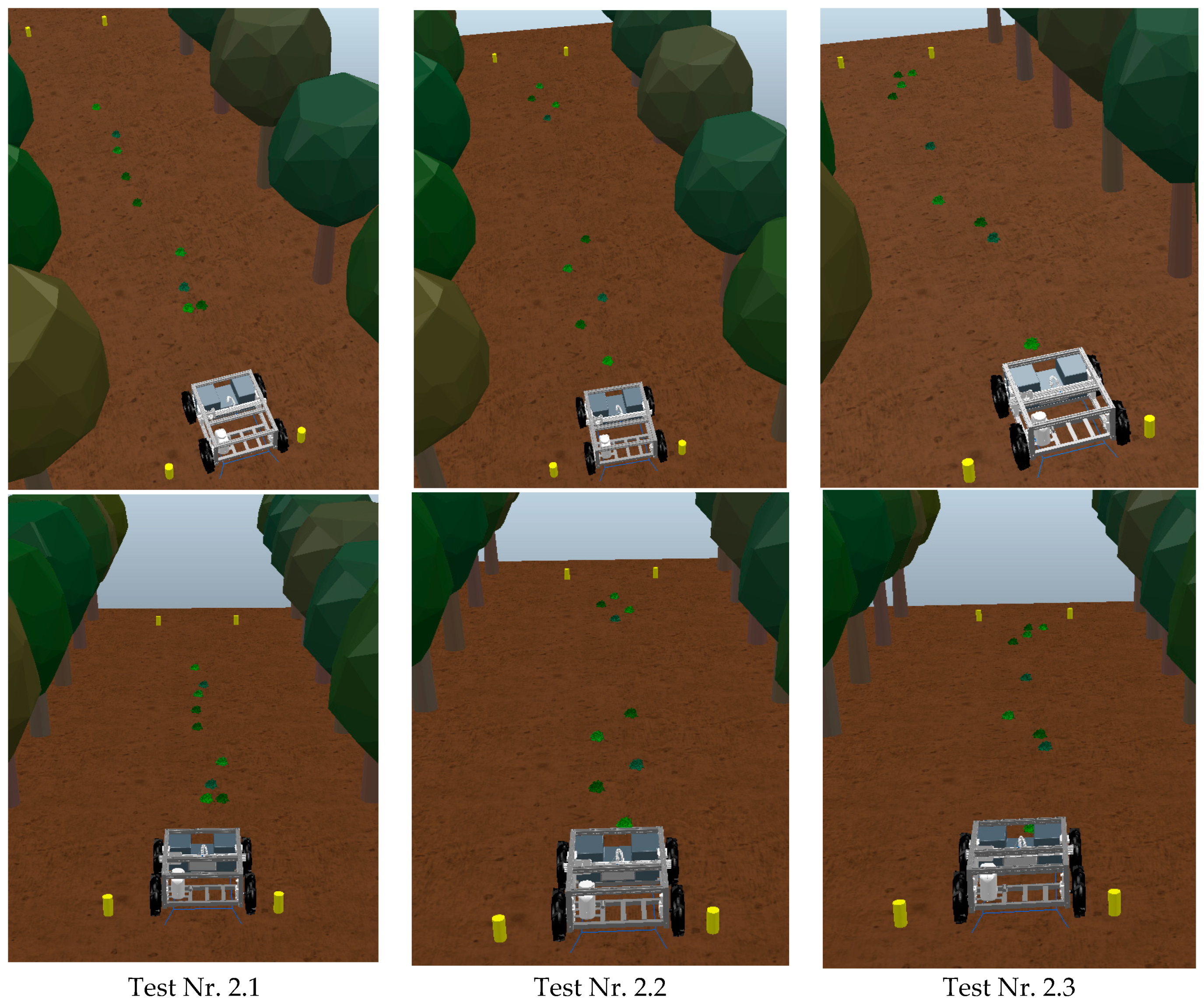
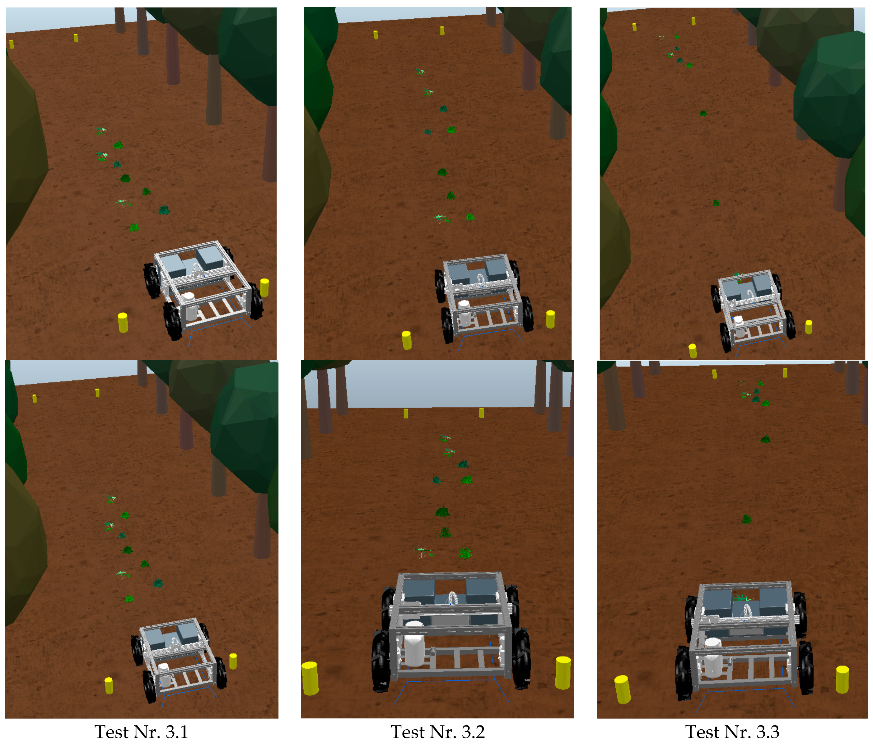
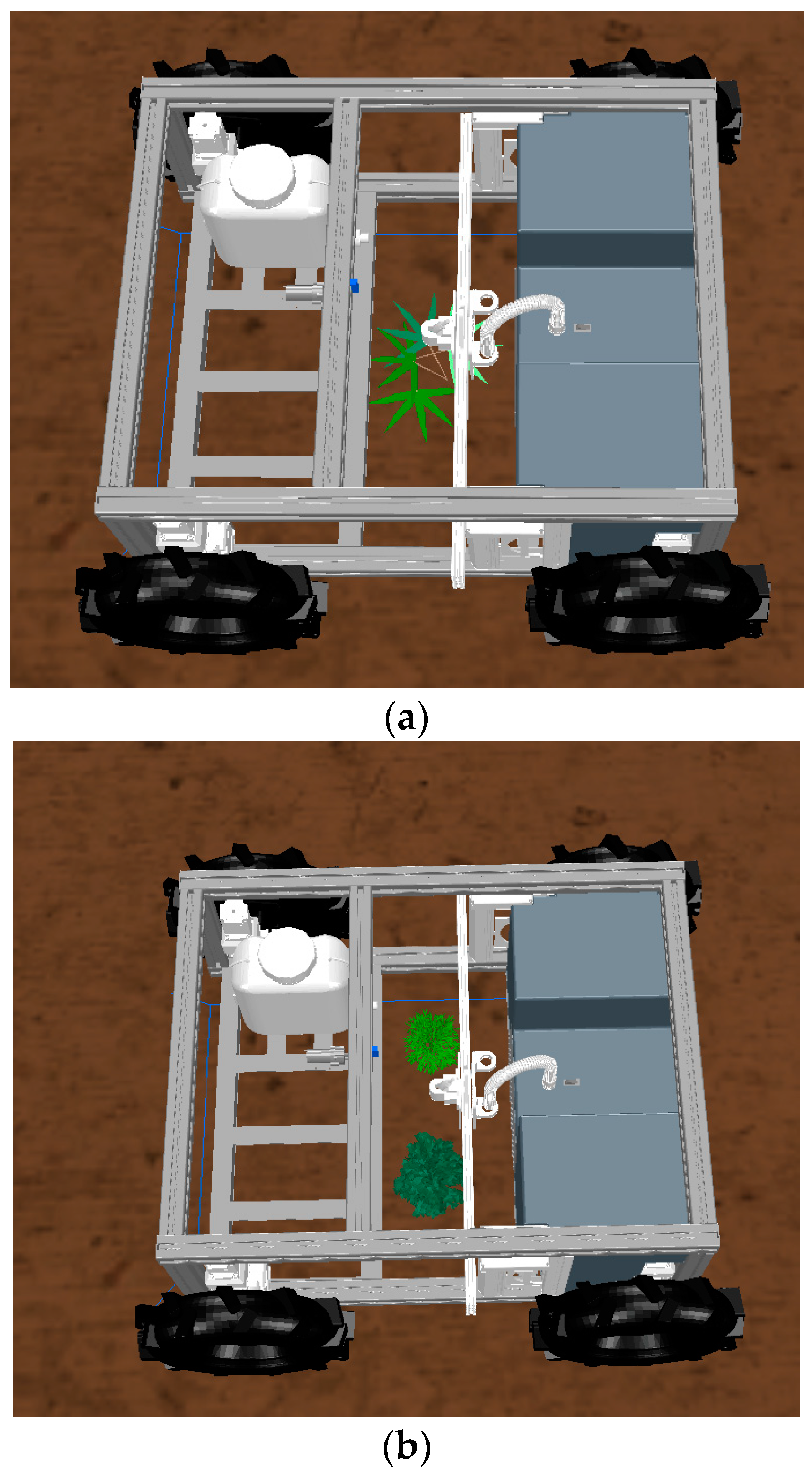
3.3. Case Study Nr. 2—Controlled Spraying

Similarly to the previous case study, in this one, a set of scenarios was also created in which the robotic rover will have to operate, and for each scenario, three tests were also performed. The difference in this case study is that the objects to be detected will have identical properties to those of the weeds, and instead of being captured, they will be sprayed. The scenarios that were defined are as follows:
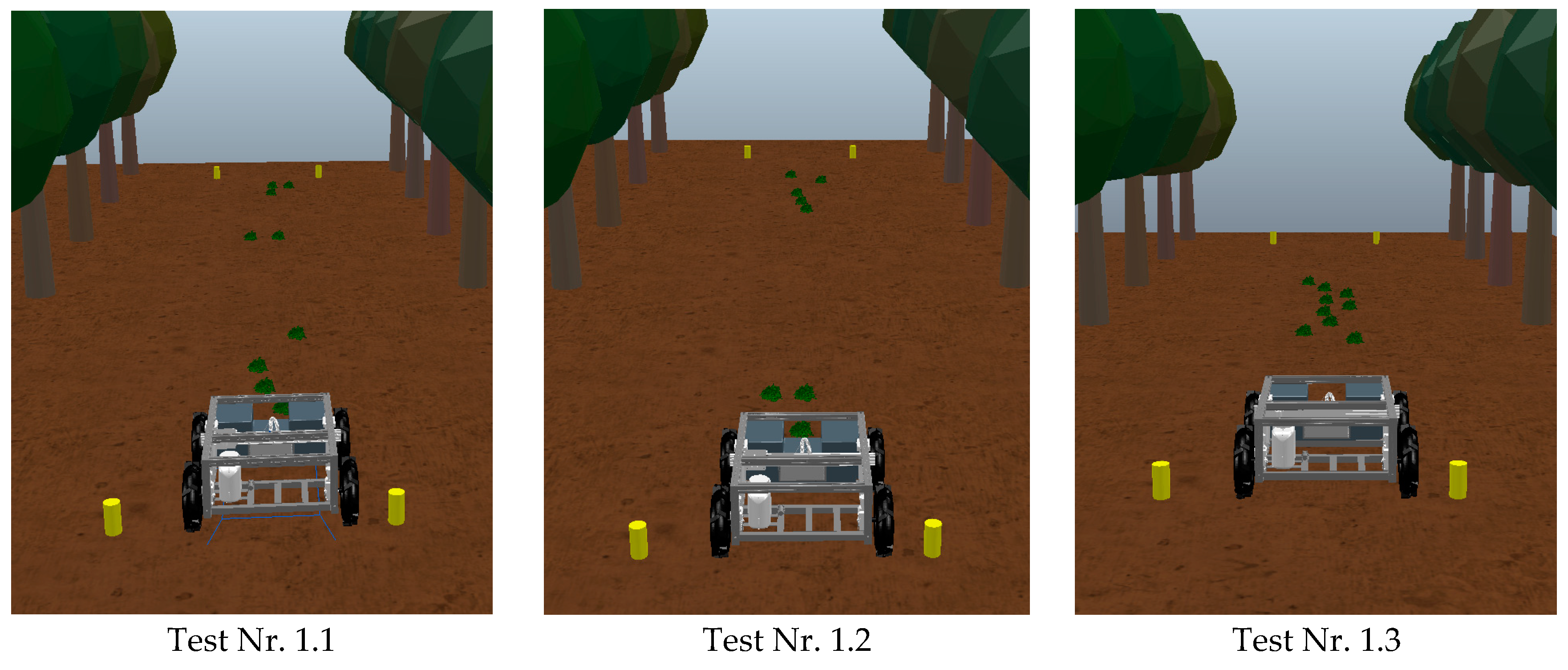
  • Scenario Nr. 1: Weeds with identical shapes and colors;
  • Scenario Nr. 2: Weeds with the same shape but with different color ranges;
  • Scenario Nr. 3: Weeds with different shapes and color ranges.
Note that the trajectory to be covered will continue to be 12 m and the number of objects to be sprayed will also be nine. Table 2 and Figure 22 show the color ranges used and the shapes that these objects may have.

3.3.1. Scenario Nr. 1

For this first scenario, the object that was used was “Weed Nr. 1” since it is the object with the highest density and, therefore, the easiest, from the start, to be detected. Regarding the color to be used, “shade Nr. 2” was chosen. In Figure 23, we can observe the positions in which the objects were placed for the three tests performed.

3.3.2. Scenario Nr. 2

In this second scenario, the “Weed Nr. 1” object was used again, with the difference being that, now, the four-color shades presented in Table 2 were used. The positions used for the three tests are represented in Figure 24.

3.3.3. Scenario Nr. 3

For this last scenario, three objects of each of the shape types shown in Figure 22 were placed. The four color ranges were also used in different objects. The positions used for the three tests are represented in Figure 25.

3.4. Results Analysis

After demonstrating the main issues that arose during the various simulations performed and also demonstrating the simulations that were performed for the two case studies, it can be concluded that the proposed algorithm was quite successful. In both case studies, the algorithm was always able to detect the objects that were intended to be captured, as well as perform the steps that followed the detection of the object.

3.4.1. Results of Case Study Nr. 1

In this case study, the detection of the objects was achieved in the different scenarios that were proposed. Including scenario Nr. 3, which would represent the greatest difficulty because all objects were different both in terms of color and size. The only difficulty identified was in capturing larger objects, especially those with diameters greater than 85 mm, and it was necessary to slightly increase the opening angle of the mechanical grab joints, as observed in Figure 26.
For the various simulations performed, in each scenario, the operating times that were required for the robotic rover to complete the object capture task were determined. These times are identified in Table 3. After observing the times, another simulation was performed to limit the maximum number of objects to be captured to five objects, which would force the platform to make a trip to the base in the middle of the object capture work.
As observed in Table 3, the fact that it required a trip to the base did not increase the total operation time excessively. Note that these operating times include the time it takes for the robotic rover to capture all the objects to reach the termination site and also the return of the robotic rover to the base.

3.4.2. Results of Case Study Nr. 2

For this second case study, detection was also achieved regardless of the scenario in question. However, to achieve these results, it was necessary to redefine the parameters of the color range to be detected, because initially, it had been set at lower values for code red and higher values for code green. However, these values had to be reduced. This situation occurred due to scenarios 2 and 3 where there were more color ranges to detect.
Another aspect that occurred in the robotic rover operation was that, if the weed to be detected was too large, there was a risk of the robotic rover spraying twice. This was more the case for “Weed Nr. 3” (Figure 27a), as it was relatively larger than the other two. However, this situation happened only sporadically. To correct this situation, we chose to add a condition to the algorithm that, whenever a weed was sprayed, the algorithm would ignore the 100 pixels around the sprayed weed. Thus, for the various tests performed, the algorithm already worked correctly; even when we had two weeds relatively close together, the algorithm could detect both and sprayed both (Figure 27b).
For this case study, the operating times required for the robotic rover to travel the entire route, detect all weeds, and return to base were also determined. These times are shown in Table 4.
For this case study, the test with a stop in the middle was not performed, because it was found in the previous study that the time difference was not substantial. Moreover, for the task at hand, one tank of the solution to be used will be enough for many uses; thus, it does not make sense to simulate this action.

4. Conclusions

The increase in food demand around the world resulted in the application of technology for increasing productivity rates. One of the most promising technologies is robotics. However, as agricultural fields are extremely dynamic environments, the development of robotics solutions for application in agricultural activities is complex and time and money consuming. A procedure that can speed up the developing process is computational simulation. This study proposes the simulation of a robotic rover operation in an orchard environment. The main goal is to create and test an algorithm that controls rover locomotion and the tasks of localized spraying and fallen fruit collection using a gripper.
After the assembly, some tests were performed in the field to evaluate its maneuverability and displacement, which is performed without major problems. However, some difficulties were encountered when transporting cargo, such as stones and fallen branches, because the robot was unable to maintain a constant speed due to the skidding of the rear wheels. The spraying system was also tested and presented no problems.
Several conclusions can be drawn. First of all, this type of simulator is undoubtedly an asset for the advancement of robotic systems, especially when there is no possibility of applying the simulation to the real world.
However, we are always left with some doubts about the results we are obtaining or because we think that the behavior of a certain component or interaction may be different in the real world. Nevertheless, the essence itself of what can happen in a given simulation is there, and often they are only small technical details that will have to be adjusted when the experiment is replicated in reality.
In this study, there are also some doubts about some of the results obtained, particularly in the case of operating speeds, which will always have to be adapted to the terrain in question and to verify whether, in the real world, the increase in speed will affect the image that much. Still, with respect to speed, we must remember that all these simulations were conducted considering a usage plan without inclinations, and it is known that agricultural fields have many inclinations and irregularities; thus, these aspects must be considered when determining the operation speed.
Regarding image processing, this is perhaps the point that arouses the greatest curiosity with respect to knowing how the platform would behave with the code created if it were applied in the real world. Moreover, this includes verifying the behavior of the hardware and the existing camera. As said in the simulation, we used the lowest resolution because we thought that higher resolutions did not produce any added value to the simulation on the contrary.
It is known that the proposed system may have some gaps in the detection of objects in the sense that performing image analysis only by color gamut and depth is somewhat ambiguous. This is because, if there is, for example, a stone that has the same color gamut and that is at the right height, because the terrain will also have several irregularities, there may be the risk of the stone being validated by the code and captured.
Regarding the operation time, if this algorithm is tested on the real platform and if all execution parameters of the various prismatic joints and the mechanical gripper are adjusted to reality and not to that of a dynamic simulation module, perhaps much improved values will be obtained, and this will not be a problem.
Note that, in this simulation, we only used the color detection function on the pixels, since the depth function was not very useful because the weeds will never have a significant height; moreover, in an agricultural field with several irregularities in the soil, it would be more difficult to analyze this parameter. Future work consists in testing the developed algorithms in the experimental platform to evaluate how precisely robotics simulation programs can replicate real-world operations. Next, new case studies will be developed in order to increase the precision of the algorithms, as well as new path planning algorithms. Finally, cooperation with drones can also be considered to identify zones with the highest density of weeds or fallen fruits, ensuring priorities for action.

Author Contributions

Conceptualization, P.D.G.; methodology, J.P.L.R. and P.D.G.; validation, P.D.G., V.N.G.J.S., and J.M.L.P.C.; formal analysis, P.D.G.; investigation, J.P.L.R. and P.D.G.; resources, J.P.L.R.; data curation, P.D.G.; writing—original draft preparation, J.P.L.R.; writing—review and editing, P.D.G., V.N.G.J.S., and J.M.L.P.C.; supervision, P.D.G.; project administration, P.D.G.; funding acquisition, P.D.G. All authors have read and agreed to the published version of the manuscript.

Funding

This research work is funded by the PrunusBOT project—autonomous controlled spraying aerial robotic system and fruit production forecast, operation no. PDR2020-101-031358 (leader), consortium no. 340, initiative no. 140, promoted by PDR2020, and co-financed by the EAFRD and the European Union under the Portugal 2020 program.

Acknowledgments

P.D.G. acknowledges Fundação para a Ciência e a Tecnologia (FCT—MCTES) for its financial support via project UIDB/00151/2020 (C-MAST). V.N.G.J.S. and J.M.L.P.C. acknowledge that this work is funded by FCT/MCTES through national funds and, when applicable, co-funded EU funds under project UIDB/50008/2020.

Conflicts of Interest

The authors declare no conflict of interest.

References

  1. Faria, S.D.N. Sensor Fusion for Mobile Robot Localization Using UWB and ArUco Markers. Master’s Thesis, Faculdade de Engenharia da Universidade do Porto, Porto, Portugal, 2021. [Google Scholar]
  2. Teixeira, G.E. Mobile Robotics Simulation for ROS Based Robots Using Visual Components. Master’s Thesis, Faculdade de Engenharia da Universidade do Porto, Porto, Portugal, 2019. [Google Scholar]
  3. Teixeira, F.M. Simulação de um Sistema Robótico de Co-Transporte. Master’s Thesis, Instituto Superior de Engenharia do Porto, Porto, Portugal, 2020. [Google Scholar]
  4. Li, Z.; Li, P.; Yang, H.; Wang, Y. Stability tests of two-finger tomato grasping for harvesting robots. Biosyst. Eng. 2013, 116, 163–170. [Google Scholar] [CrossRef]
  5. Telegenov, K.; Tlegenov, Y.; Shintemirov, A. A low-cost open-source 3-D-printed three-finger gripper platform for research and educational purposes. IEEE Access 2015, 3, 638–647. [Google Scholar] [CrossRef]
  6. Weber, P.; Rueckert, E.; Calandra, R.; Peters, J.; Beckerle, P. A low-cost sensor glove with vibrotactile feedback and multiple finger joint and hand motion sensing for human-robot interaction. In Proceedings of the 2016 25th IEEE International Symposium on Robot and Human Interactive Communication (RO-MAN), New York, NY, USA, 26–31 August 2016; pp. 99–104. [Google Scholar]
  7. Taheri, H.; Rowe, J.B.; Gardner, D.; Chan, V.; Gray, K.; Bower, C.; Reinkensmeyer, D.J.; Wolbrecht, E.T. Design and preliminary evaluation of the FINGER rehabilitation robot: Controlling challenge and quantifying finger individuation during musical computer game play. J. Neuroeng. Rehabil. 2014, 11, 10. [Google Scholar] [CrossRef] [Green Version]
  8. Edlerman, E.; Linker, R. Autonomous multi-robot system for use in vineyards and orchards. In Proceedings of the 2019 27th Mediterranean Conference on Control and Automation (MED), Akko, Israel, 1–4 July 2019; pp. 274–279. [Google Scholar]
  9. Lepej, P.; Rakun, J. Simultaneous localisation and mapping in a complex field environment. Biosyst. Eng. 2016, 150, 160–169. [Google Scholar] [CrossRef]
  10. Blok, P.M.; van Boheemen, K.; van Evert, F.K.; IJsselmuiden, J.; Kim, G.H. Robot navigation in orchards with localization based on Particle filter and Kalman filter. Comput. Electron. Agric. 2019, 157, 261–269. [Google Scholar] [CrossRef]
  11. Chou, H.-Y.; Khorsandi, F.; Vougioukas, S.G.; Fathallah, F.A. Developing and evaluating an autonomous agricultural all-terrain vehicle for field experimental rollover simulations. Comput. Electron. Agric. 2022, 194, 106735. [Google Scholar] [CrossRef]
  12. Basiri, A.; Mariani, V.; Silano, G.; Aatif, M.; Iannelli, L.; Glielmo, L. A survey on the application of path-planning algorithms for multi-rotor UAVs in precision agriculture. J. Navig. 2022, 1, 1–20. [Google Scholar] [CrossRef]
  13. Wang, S.; Dou, W.; Li, T.; Han, Y.; Zhang, Z.; Chen, J. Path Planning Optimization and Motion Control of a Greenhouse Unmanned Ground Vehicle. Lect. Notes Electr. Eng. 2022, 644, 5145–5156. [Google Scholar]
  14. Jiang, Y.; Xu, X.; Zhang, L.; Zou, T. Model Free Predictive Path Tracking Control of Variable-Configuration Unmanned Ground Vehicle. ISA Trans. 2022. Available online: https://pubmed.ncbi.nlm.nih.gov/35148886/ (accessed on 10 February 2022). [CrossRef]
  15. Wu, Y.; Li, C.; Yuan, C.; Li, M.; Li, H. Predictive Control for Small Unmanned Ground Vehicles via a Multi-Dimensional Taylor Network. Appl. Sci. 2022, 12, 682. [Google Scholar] [CrossRef]
  16. Bayar, G.; Bergerman, M.; Koku, A.B.; Konukseven, E.I. Localization and control of an autonomous orchard vehicle. Comput. Electron. Agric. 2015, 115, 118–128. [Google Scholar] [CrossRef] [Green Version]
  17. Cutulle, M.A.; Maja, J.M. Determining the utility of an unmanned ground vehicle for weed control in specialty crop systems. Ital. J. Agron. 2021, 16, 365–478. [Google Scholar] [CrossRef]
  18. Du, Y.; Mallajosyula, B.; Sun, D.; Chen, J.; Zhao, Z.; Rahman, M.; Quadir, M.; Jawed, M.K. A Low-cost Robot with Autonomous Recharge and Navigation for Weed Control in Fields with Narrow Row Spacing. In Proceedings of the IEEE/RSJ International Conference on Intelligent Robots and Systems (IROS), Prague, Czech Republic, 27 September–1 October 2021; pp. 3263–3270. [Google Scholar]
  19. Machleb, J.; Peteinatos, G.G.; Sökefeld, M.; Gerhards, R. Sensor-Based Intrarow Mechanical Weed Control in Sugar Beets with Motorized Finger Weeders. Agronomy 2021, 11, 1517. [Google Scholar] [CrossRef]
  20. Kurpaska, S.; Bielecki, A.; Sobol, Z.; Bielecka, M.; Habrat, M.; Śmigielski, P. The Concept of the Constructional Solution of the Working Section of a Robot for Harvesting Strawberries. Sensors 2021, 21, 3933. [Google Scholar] [CrossRef]
  21. Rysz, M.W.; Mehta, S.S. A risk-averse optimization approach to human-robot collaboration in robotic fruit harvesting. Comput. Electron. Agric. 2021, 182, 106018. [Google Scholar] [CrossRef]
  22. Cruz Ulloa, C.; Krus, A.; Barrientos, A.; del Cerro, J.; Valero, C. Robotic Fertilization in Strip Cropping using a CNN Vegetables Detection-Characterization Method. Comput. Electron. Agric. 2022, 193, 106684. [Google Scholar] [CrossRef]
  23. Mohapatra, B.N.; Jadhav, R.V.; Kharat, K.S. A Prototype of Smart Agriculture System Using Internet of Thing Based on Blynk Application Platform. J. Electron. Electromed. Eng. Med. Inform. 2022, 4, 24–28. [Google Scholar] [CrossRef]
  24. Mammarella, M.; Comba, L.; Biglia, A.; Dabbene, F.; Gay, P. Cooperation of Unmanned Systems for Agricultural Applications: A Theoretical Framework. Biosyst. Eng. 2021. Available online: https://www.sciencedirect.com/science/article/pii/S1537511021002750 (accessed on 17 December 2021). [CrossRef]
  25. Aslan, M.F.; Durdu, A.; Sabanci, K.; Ropelewska, E.; Gültekin, S.S. A Comprehensive Survey of the Recent Studies with UAV for Precision Agriculture in Open Fields and Greenhouses. Appl. Sci. 2022, 12, 1047. [Google Scholar] [CrossRef]
  26. Veiros, A.F.R. Sistema Robótico Terrestre Para Apoio a Atividades de Manutenção de Solo em Pomares de Prunóideas. Master’s Thesis, Universidade da Beira Interior, Covilhã, Portugal, 2020. [Google Scholar]
  27. Vigneault, C.; Bechar, A. Agricultural robots for field operations. Part 2: Operations and systems. Biosyst. Eng. 2017, 153, 110–128. [Google Scholar]
  28. Oerke, E.C.; Dehne, H.W. Safeguarding production—losses in major crops and the role of crop protection. Crop Prot. 2004, 23, 275–285. [Google Scholar] [CrossRef]
  29. Tavares, N.; Gaspar, P.D.; Aguiar, M.L.; Mesquita, R.; Simões, M.P. Robotic arm and gripper to pick fallen peaches in the orchards. In Proceedings of the X International Peach Symposium, Naoussa, Greece, 30 May–3 June 2022. [Google Scholar]
  30. Coppelia Robotics Ltd Robot Simulator CoppeliaSim. Available online: https://www.coppeliarobotics.com/ (accessed on 21 October 2021).
  31. Miranda, L. Analysis and Simulation of AGVS Routing Strategies Using V-REP. 2017. Available online: https://www.semanticscholar.org/paper/Analysis-and-simulation-of-AGVS-routing-strategies-Miranda/1769570e18411d9c0fec420221eda444fb03fbda (accessed on 12 January 2022).
  32. Shamshiri, R.R.; Hameed, I.A.; Pitonakova, L.; Weltzien, C.; Balasundram, S.K.; Yule, I.J.; Grift, T.E.; Chowdhary, G. Simulation software and virtual environments for acceleration of agricultural robotics: Features highlights and performance comparison. Int. J. Agric. Biol. Eng. 2018, 11, 12–20. [Google Scholar] [CrossRef]
  33. Simões, M.P.; Barateiro, A.; Duarte, A.C.; Dias, C.; Ramos, C.; Alberto, D.; Ferreira, D.; Calouro, F.; Vieira, F.; Silvino, P.; et al. +Pessego. Guia Prático da Produção; Centro Operativo e Tecnologíco Hortofrutícola Nacional: Porto, Portugal, 2016; Volume I, ISBN 9789728785048. Available online: https://www.researchgate.net/profile/Maria-Paula-Simoes/publication/344614906_Cap_03-36_Manutencao_solo_pessegueiros_Atividade_enzimatica/links/5f84827e458515b7cf7a7845/Cap-03-36-Manutencao-solo-pessegueiros-Atividade-enzimatica.pdf (accessed on 12 January 2022).
  34. Simões, M.P.A.F. A Fertilização Azotada em Pessegueiros: Influência no Estado de Nutrição, Produção e Susceptibilidade a Phomopsis Amygdali. Available online: https://www.repository.utl.pt/handle/10400.5/1591?locale=en (accessed on 12 January 2022).
  35. Leopoldo Armesto DYOR. Available online: http://dyor.roboticafacil.es/en/ (accessed on 27 October 2021).
  36. Universitária, I. O que são Padrões de Cores RGB e CMYK?—Imprensa Universitária. Available online: https://imprensa.ufc.br/pt/duvidas-frequentes/padrao-de-cor-rgb-e-cmyk/ (accessed on 27 October 2021).
Figure 1. Exploded view of the robot.
Electronics 11 00790 g001
Figure 2. Isometric perspective of the robot.
Electronics 11 00790 g002
Figure 3. Robotic platform in operation in the field.
Electronics 11 00790 g003
Figure 4. Gripper work envelope on the Cartesian axis (represented with shadow and blue lines).
Electronics 11 00790 g004
Figure 5. Final gripper prototype: isometric view.
Electronics 11 00790 g005
Figure 6. Simulator graphical interface.
Electronics 11 00790 g006
Figure 7. Final layout of the robotic platform loaded into the simulator.
Electronics 11 00790 g007
Figure 8. Recreation of the mechanical gripper in the simulator.
Electronics 11 00790 g008
Figure 9. Installing the camera on the robotic platform.
Electronics 11 00790 g009
Figure 10. Vision sensor zones: Zone A Electronics 11 00790 i001—Object detection; Zone B Electronics 11 00790 i002—Picking object.
Electronics 11 00790 g010
Figure 11. Flowchart for controlling the robotic platform.
Electronics 11 00790 g011
Figure 12. Flowchart for object picking.
Electronics 11 00790 g012
Figure 13. Definition of a compass. Legend: Line: Electronics 11 00790 i003; Interline: Electronics 11 00790 i004.
Electronics 11 00790 g013
Figure 14. Final layout used in the robotic simulations.
Electronics 11 00790 g014
Figure 15. Introduction of objects for capture in the simulation.
Electronics 11 00790 g015
Figure 16. Examples of the mechanical gripper not being aligned with the object.
Electronics 11 00790 g016
Figure 17. Sequence of the robotic rover in the process of capturing an object.
Electronics 11 00790 g017
Figure 18. Behavior of the objects to be captured with the dynamic simulation module Bullet 2.78.
Electronics 11 00790 g018
Figure 19. Tests performed for scenario Nr. 1.
Electronics 11 00790 g019
Figure 20. Tests performed for scenario Nr. 2.
Electronics 11 00790 g020aElectronics 11 00790 g020b
Figure 21. Tests performed for scenario Nr. 3.
Electronics 11 00790 g021
Figure 22. Types of shapes used in the representation of weeds.
Electronics 11 00790 g022
Figure 23. Tests performed for scenario Nr. 1.
Electronics 11 00790 g023aElectronics 11 00790 g023b
Figure 24. Tests performed for scenario Nr. 2.
Electronics 11 00790 g024
Figure 25. Tests performed for scenario Nr. 3.
Electronics 11 00790 g025
Figure 26. Example of capturing objects with larger dimensions.
Electronics 11 00790 g026
Figure 27. Weed detection. (a) Weed Nr. 3 spraying. (b) Spraying of various weeds.
Electronics 11 00790 g027
Table 1. Technical specifications of the robotic rover for agricultural applications (R2A2).
Robot SpecificationValue
Approximate weight90 kg
Payload15 kg
Maximum speed1.4 m/s
Acceleration1 m/s2
Length1200 mm
Width1050 mm
Height500 mm
Table 2. Color code used.
ItemColor Code
RedGreenBlue
Use Plan0.3760.2580.164
Yellow peach0.9330.7720.043
Orange peach0.9760.5840.082
Reddish peach0.9920.3090.081
Toning Weed Nr. 10.2340.7750.074
Toning Weed Nr. 20.0310.4730.030
Toning Weed Nr. 30.1910.5090.331
Toning Weed Nr. 40.2080.7400.207
Table 3. Elapsed times in performing the various simulations of case study Nr. 1.
Case Study Nr. 1Time without StopTime with Stop
Scenario Nr. 1Test Nr. 1.13 min, 10 s3 min, 14 s
Test Nr. 1.23 min, 10 s3 min, 16 s
Test Nr. 1.33 min, 10 s3 min, 26 s
Scenario Nr. 2Test Nr. 2.13 min, 11 s3 min, 19 s
Test Nr. 2.23 min, 10 s3 min, 38 s
Test Nr. 2.33 min, 08 s3 min, 14 s
Scenario Nr. 3Test Nr. 3.13 min, 13 s3 min, 21 s
Test Nr. 3.23 min, 10 s3 min, 16 s
Test Nr. 3.33 min, 14 s3 min, 20 s
Table 4. Elapsed times in performing the various simulations of case study Nr. 2.
Case Study Nr. 2Time
Scenario Nr. 1Test Nr. 1.11 min, 08 s
Test Nr. 1.21 min, 06 s
Test Nr. 1.31 min, 05 s
Scenario Nr. 2Test Nr. 2.11 min, 12 s
Test Nr. 2.21 min, 09 s
Test Nr. 2.31 min, 06 s
Scenario Nr. 3Test Nr. 3.11 min, 09 s
Test Nr. 3.21 min, 05 s
Test Nr. 3.31 min, 05 s
Publisher’s Note: MDPI stays neutral with regard to jurisdictional claims in published maps and institutional affiliations.

