1. Introduction
Recently, grid-connected inverters (GCIs) for interfacing between power sources and the unity grid are widely used to facilitate the renewable energy generation system and the smart grid [
1]. Because a power conversion system is expected to operate with high efficiency, flexibility, and reliability, the GCI should be controlled by a robust control algorithm to stabilize the system even under severe non-ideal conditions [
2,
3]. In addition, to meet the power quality standard as mentioned in [
4], distributed generation (DG) power systems are required to provide high-quality currents into the grid, which is guaranteed by the current controller of the GCI. The current controller of the GCI system should maintain the system stability despite various negative impacts from internal uncertainties as well as external disturbances [
5]. Particularly, internal uncertainties are caused by inductor-capacitor-inductor (LCL) filter parameter variations due to the temperature or the aging-induced effect as well as the weak grid condition. The external disturbances are primarily caused by unexpected grid fault events in the unity grid [
6,
7].
The pulse width modulation (PWM) with a high switching frequency is widely adopted in inverter topologies to maximize the efficiency. The inverter filters in type of inductor (L), inductor–capacitor (LC), or LCL are an essential component to suppress switching ripples of injected currents in inverter structures. The LCL filter provides a better harmonic suppression capability and reduces the filter inductor size as well as hardware cost in comparison with the other filter types. However, the complicated dynamics and the resonance phenomenon of the LCL-filtered inverter system pose challenges for the controller design to achieve the objectives such as the reference tracking and disturbance rejection [
8]. As a result, effective damping methods should also be considered in the design process of the high-performance current controller in an LCL-filtered GCI system [
9].
In addition to the resonance phenomenon due to the use of LCL filters, several factors should be considered in designing the current controller for GCI. The main factors affecting the grid-injected current quality are the internal disturbances caused by the parameter uncertainty as well as the external disturbances such as the grid impedance variation, grid frequency variation, and grid imbalanced and distorted voltages. To deal with this issue, the robust control schemes have been investigated to ensure the system performance under both parameter variations and external disturbances from the grid environment. The proportional-integral (PI) and the proportional resonance (PR) controllers are commonly deployed for the reference tracking and harmonic disturbance rejection in GCI. The internal model (IM) suggested by Francis and Woham [
10] has been developed to design the PI and PR controllers in the state-space representation. In this regard, there have been several research works to use the IM approach in the current control design. However, the design based on the IM structure requires the selection of appropriate controller gains in order to stabilize the system, and to ensure desirable steady-state and transient performances [
11,
12,
13].
The linear quadratic regulator (LQR) has also been presented to produce the optimized gains of the controller by minimizing the cost function with the weighting factors [
11,
14]. In comparison with the pole placement method in [
6], the LQR method offers the optimal state feedback gain set by adjusting the weighting factors to achieve a satisfactory system response. However, it is worth mentioning that the LQR-based controller often requires the knowledge and experience of user to find appropriate weighting factors. In the other approaches, the studies in [
13,
15] solve the linear matrix inequality (LMI) derived from the condition of stability in the Lyapunov theorem to obtain the controller gain optimally. Meanwhile, the LMI algorithm is an effective and powerful tool to design a robust controller by taking the system uncertainties into consideration. The task of optimizing the cost function of the LMI over the infinite horizon becomes challenging when the system model includes polytopic uncertainty. Another study integrates the LMI with the LQR method, in which the upper boundary of the cost function is reduced with the infinite horizon at each sampling period [
12]. This work presents a current controller to deal with distorted grid voltages, grid frequency variation, and parameter uncertainties in the LCL filter. Even though this study provides good results under several external disturbances and system uncertainties, the unexpected grid environment such as imbalanced grid voltages still degrades the control operations.
The model predictive control (MPC) is increasingly attracting the attention of researchers due to its simple concept, good reference tracking, and excellent constraint-handling ability. In general, the MPC is solved online during each sampling period to compute the optimal control inputs based on the predicted future outputs. Instead of predicting the model of the system for the control input at each sampling period, another one of the MPC-based approaches in [
16,
17,
18] selects proper switching states to apply desired reference voltages. These control schemes are straightforward and have no excessive computational load. However, they take a very high sampling frequency and do not present the analysis of robustness or stability. Furthermore, the MPC scheme is known to be sensitive against parameter discrepancies, which may lead to performance degradation. To address this issue, the approaches in [
19,
20] combine the LMI-based optimization with the MPC to implement an optimal controller with robustness against parametric uncertainties. In addition, the LMI-based MPC optimization schemes have been applied to achieve a rapid convergence rate of the desired states and to optimally obtain the controller gains from the stability conditions [
21,
22,
23,
24]. However, the MPC schemes mentioned above do not take into consideration the grid imbalance and frequency fluctuations as the main causes of disturbance during grid failures.
The controller of the LCL-filtered inverter has been gathering several research attentions to reduce the total cost and hardware complexity. The sensors in the inverter system contribute greatly to increase the overall system cost. This issue encourages the research topics to reduce the number of sensing devices while maintaining the availability of full-state variables. The state feedback controller approach still requires additional sensors to measure full-state variables. The full-state observer is a good approach to reduce the need of current and voltage sensors for inverter-side current and capacitor voltage, respectively, as presented in [
11]. The full-state observer uses the grid-side currents, grid voltages, and the control input information to estimate full-state variables without harming the system of reliability. As a practical way of designing a grid-connected inverter for DG applications, an integral state feedback control and state observer are designed in a discrete-time domain [
6]. Even though the above study presents a systematic controller design methodology for an LCL-filtered inverter, it does not consider the control robustness against the grid voltage imbalance and several parameter uncertainties. In [
6,
25,
26], the authors deploy the predictive-type observer to estimate inverter state variables in the synchronous reference frame (SRF). Obviously, the observer performance is maintained well under ideal grid conditions. To enhance the accuracy of the estimated states under distorted grid environment, the studies in [
13,
14,
27] construct the current-type observer, which ensures the reliability of the full-state feedback controller.
In this paper, an LMI-based MPC is proposed to control an LCL-filtered GCI under unexpected grid and system uncertainties, which guarantees a system stability and reliable operation. The variation of the grid impedance is also considered by means of the LMI method. Even though the evaluation results of the conventional MPC scheme demonstrate its effectiveness under several test conditions, it is difficult to determine an optimized weighting matrix of the MPC cost function. To overcome this problem, the MPC combining the LMI-based optimization is applied in this paper to obtain a weighting matrix of the MPC cost function [
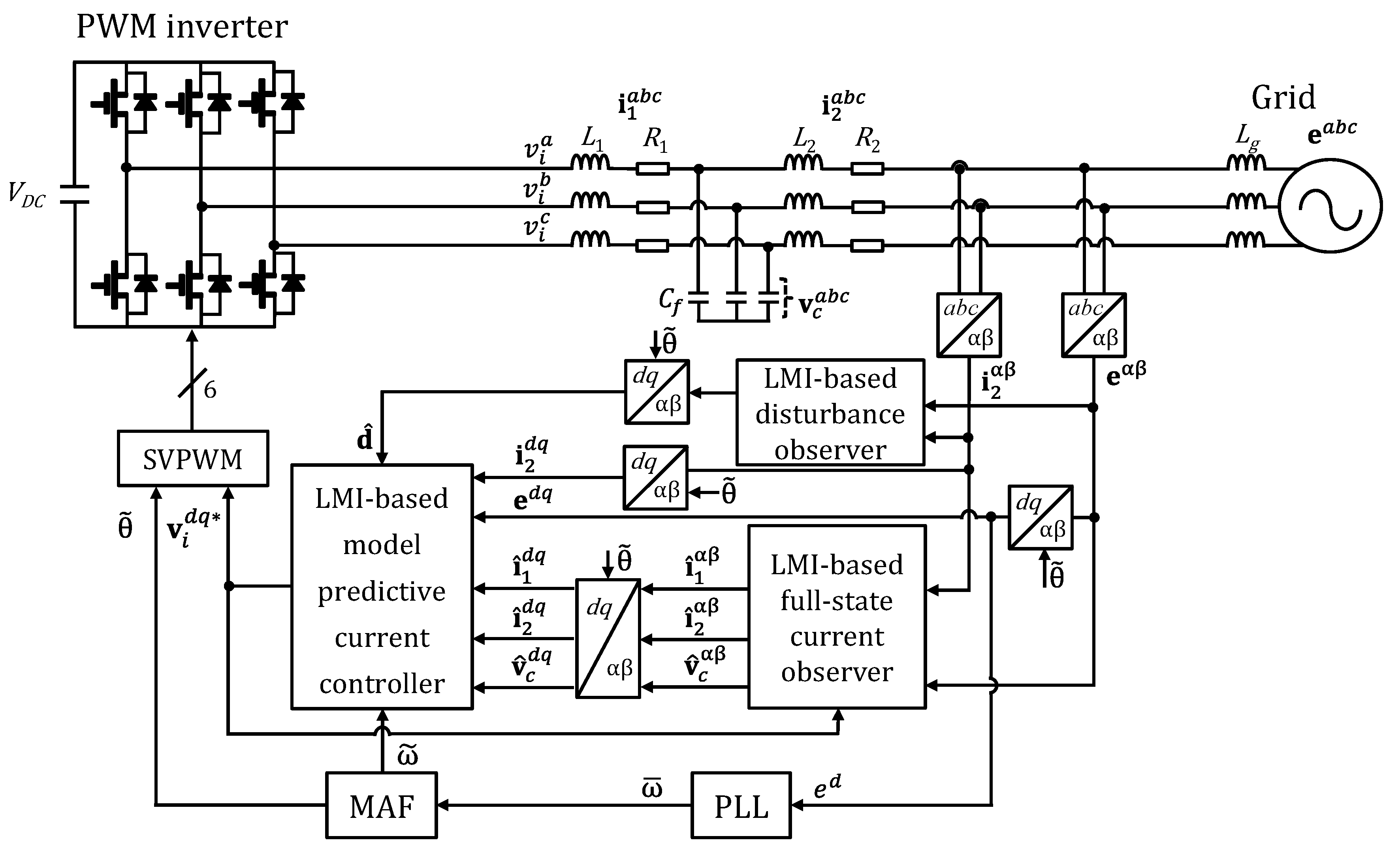
21]. The LMI-based MPC approach is combined with the LQR method to determine the boundaries of the Lyapunov function within a certain range and to guarantee the stability under severe parameter uncertainty condition. In the proposed scheme, the system states are estimated by the LMI-based current-type observer in the stationary reference frame. Since the system model in the stationary frame does not include the frequency information in the system matrix, the model discretization can be performed by an offline method, and the observer estimating performance is not degraded even under grid frequency variation. The MPC scheme is combined with the disturbance observer to eliminate offset error, which improves the reference tracking performance. To ensure high-quality grid-injected currents under distorted grid environment, the multiple grid frequency-adaptive PR controllers are constructed in parallel at the 6th and 12th orders in SRF, which successfully attenuates the harmonics in 5th, 7th, 11th, and 13th in the
abc frame, respectively [
28]. For this purpose, the grid frequency information is updated online to the PR controllers to ensure harmonic suppression performance even under grid-frequency deviation. Since the frequency extracted from the existing phase lock loop (PLL) shows fluctuations under harmonically distorted grid voltages, a moving average filter (MAF) is adopted to eliminate this fluctuation, and the filtered grid frequency information is used for the PR controllers [
29]. In comparison with the other studies, the proposed control method ensures highly robust control performance under grid voltage imbalance, parameter uncertainties, and frequency variation. In addition, the proposed approach achieves a robust active damping even for the grid impedance variation without the need of considering further damping method. The control design step is systematic and straightforward. Furthermore, unlike the conventional schemes, the proposed controller does not require an integral term and the 2nd harmonic compensation term to obtain a good reference tracking performance under grid imbalanced condition, which contributes to the reduction of the controller complexity by decreasing the order of the controller model. In the proposed scheme, an online computation process is avoided by obtaining the control gains through an offline computing method. To verify the effectiveness of the proposed LMI-based MPC control scheme, the simulations and experiments are carried out by using a prototype three-phase GCI. The comprehensive simulation and experimental results clearly demonstrate the robustness of the proposed current controller under various adverse test conditions under unexpected grid and system uncertainties.
3. Proposed LMI-Based Model Predictive Current Control
In general, the MPC produces the optimal control performance by minimizing the cost function of system state variables at the current and future timeslots. However, on-line implementation causes high computational burden in the digital processor. Furthermore, the challenging point of the MPC scheme is to determine the optimum weighting matrix of the MPC cost function and to stabilize the system under parameter uncertainties, as well as grid disturbances.
To overcome such limitations in this paper, the excessive online computation of the conventional MPC is avoided by means of an offline computing process, to obtain the control gains. In addition, the MPC is combined with the LMI tool to ensure the robustness against parameter uncertainty and grid disturbances, by satisfying output performance.
3.1. LMI-Based Model Predictive Current Control
By successively applying (16), the prediction model of the system is expressed as follows:
where
The predictive model (22) is utilized to predict the control input u(k). The predicted future time steps are represented by the length of the prediction horizon N, which indicates the distance to predict the future controller.
Generally, the MPC scheme requires the information of system reference states that are derived from the grid-side reference currents
and the measured grid-side voltages
. It is obvious that in the SRF, the steady-state reference vector
is equal to the next step value
. Similarly, the next step reference input vector
is equal to
. From (2) to (7), taking the time derivative terms of the steady-state reference variables equal to zero leads to
where
denotes the estimated disturbance vector,
and
are the inverter-side current references, and
and
are the capacitance voltage references in the SRF. In (24)–(29), the disturbance vector
d in (2)–(7) is replaced by the
and
is replaced with
. Equations (24)–(29) are represented in the state-space form as
where
denotes the reference state vector,
denotes the reference input vector, and the system matrices are expressed as
The cost function is calculated based on the difference between the system states and the reference states, as follows:
where
and
are symmetric positive definite matrices. The optimal control input
is found by equating the first derivative of
with respect to
u(
k) to zero as below
Then, the control input can be deduced from (33) and (34) as
or
where
.
The reference tracking objective is achieved by minimizing the cost function, in which the cost function is constructed from the errors between the reference and actual state variables. In the conventional state feedback structure in [
13], the integral term and resonant term at 2nd harmonic are augmented into the state feedback system to ensure the tracking performance under imbalanced grid voltages, which raises concern about computational burden. On the other hand, in the proposed control scheme, a good reference tracking performance is maintained under balanced or imbalanced grid environment by the control input (36), without any extra control terms.
To guarantee the robustness under parameter variations, a combination of the MPC method and the LMI optimization is devised in this paper by obtaining a weight matrix
of the MPC cost function based on the LMI optimization method. For this purpose, a Lyapunov function is constructed as follows:
If the Lyapunov function satisfies V(k + 1) < V(k), the system is stable in the sense of Lyapunov theory.
Suppose that
V(
k) satisfies the following inequality (38) and that the cost function
of the LQR derives the upper boundary of the Lyapunov function within a certain range for the robust stability as
or in the LMI form
where
and
are the weighting matrices of the LQR. Moreover, the cost function
of the LQR can be expressed as
For utilizing the LMI technique, the symmetric, positive, definite matrix
is multiplied on the left and right sides of (39) to yield
Utilizing Schur complement to (41) yields
for
I = 1, 2,
, 8.
To minimize the upper boundary, the sum of Lyapunov difference in (38) is calculated from
k = 0 to
k =
, as follows:
Equation (43) is represented as
, in which
denotes the cost function of the LQR for the infinite horizon (
N =
). If the system controller is stable, it can be assumed that
and
. Then, with
denoting the upper bound of
V(0), the following condition holds
or
Accordingly, the optimal weighting matrix
should be established by solving the optimization problem, as follows:
where
is utilized as the weighting matrix of the MPC in (35). When calculating the optimal weighting matrix
, the condition of (46) should be maintained, which ensures the robust stability of the system under the variations of
L1,
L2, and
Cf.
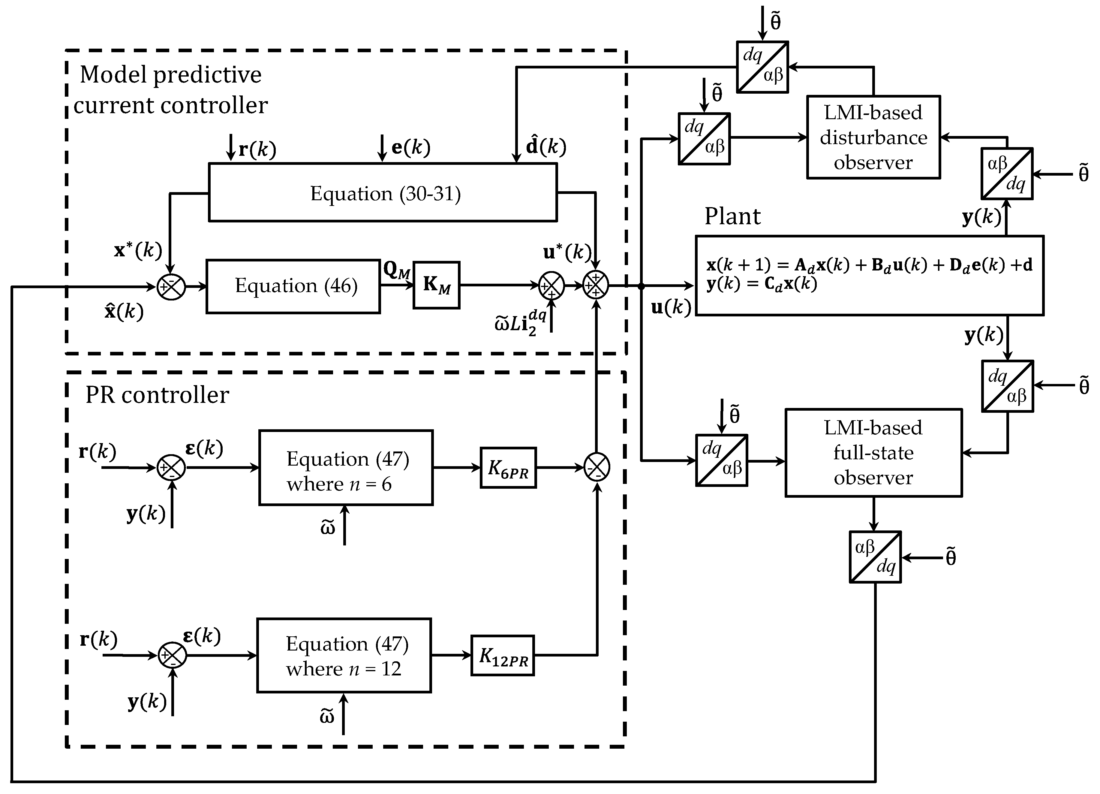
Figure 2 shows the block diagram of the proposed LMI-based model predictive current controller. In this figure,
is the grid-side current error vector;
is the MPC gain; and
are the PR gains for 6th and 12th order harmonics, respectively, which are presented in the next subsection.
3.2. Distorted Harmonic Compensators
In order to compensate for the negative effects of the distorted grid on the injected currents, the PR controllers are commonly constructed. By means of the two PR controllers tuned at 6th and 12th orders in the SRF, the four harmonic components of the 5th, 7th, 11th, and 13th orders in phase currents are effectively attenuated without much computational burden. In this study, the frequency-adaptive PR controllers, which are parallelly constructed with the proposed MPC, are expressed as follows [
29]:
where
n = 6, and 12 is the distorted harmonic order.
3.3. Frequency Detection under Distorted Grid Voltages
The conventional PLL degrades the capability of the PR controllers to compensate for distorted harmonics due to the frequency fluctuations under distorted grid voltages. Obviously, the accurate frequency information is essential to constitute the resonant controllers. To mitigate the negative effect of grid disturbances on the detected grid frequency, the SRF-PLL scheme is incorporated with the MAF represented, as follows [
13]:
where
M denotes the number of samples in a window length,
is the grid angular frequency from the SRF-PLL, and
is the filtered grid angular frequency. To compensate for any phase delay caused by the MAF, an adaptive delay compensator
C is used. The phase-lead compensator of MAF is represented as
3.4. LMI-Based Current-Type Full-State and Disturbance Observer
For implementing the proposed controller, the full-state current observer is adopted to estimate all the states, such as the grid-side currents i2, the inverter-side currents i1, and the capacitor voltages vc without additional sensors. The inverter system model in the SRF requires the information on the grid angular frequency. On the other hand, since there is no need to take into account the grid frequency information in the stationary reference frame, the inverter model can be easily discretized by the offline method in the circumstance of frequency variation.
Thus, the current-type full-state observer is constructed in the stationary reference frame in this paper as
where
is the current-type full-state observer gain set. The first estimated state
is computed by estimated state, control input, and inverter-side voltage at the current time step
k. Then, the estimated state
is obtained by the most recent measurements of
y and estimation
at the next time step (
k + 1)
.
In addition, to reject negative effects on the performance of the control system, the disturbance observer is constructed in the stationary reference frame as
where
is the disturbance observer gain set. To systematically derive the optimized observer gain, the full-state observer in (50)–(51) and disturbance observer in (52) are augmented as follows:
In this study, the proposed disturbance observer estimates the grid voltage disturbance and model uncertainties of the GCI. The Lyapunov function
(
k) is represented based on the augmented structure in (53), as follows:
where the weighting matrix
W is positive definite. For the stability of the observer, the Lyapunov function
(
k) requires the condition as
or
To quickly reduce the Lyapunov function, the convergence rate
(0 <
< 1) is inserted into (56) as
or
where
=
and
. Multiplying
on the left- and right-hand sides of (58) yields
where
=
and
=
Applying the Schur complement to (59) yields
Accordingly, the full-state observer gain and the disturbance observer gain should be established by minimizing in the LMI optimization problem in (60).
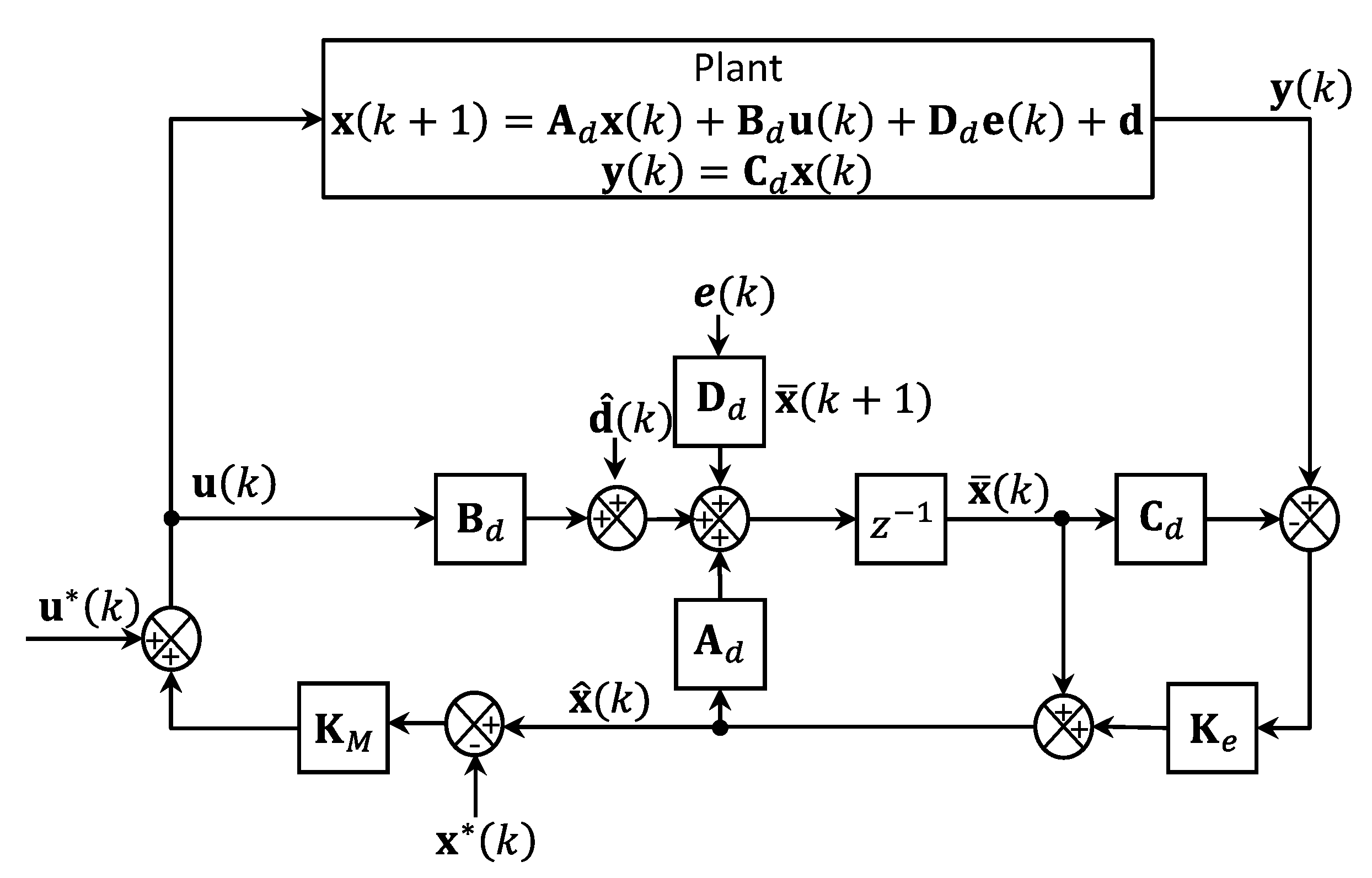
Figure 3 presents the block diagram of the LMI-based current-type full-state observer. In this figure, the estimated state vector
is used to configure the state feedback control inputs of the MPC.
4. Simulation Results
In this section, the simulation results of the proposed control performance are presented using PSIM software. To verify the robustness of the proposed controller, the eigenvalue locations of the control system are investigated in the
z-domain in Matlab environment.
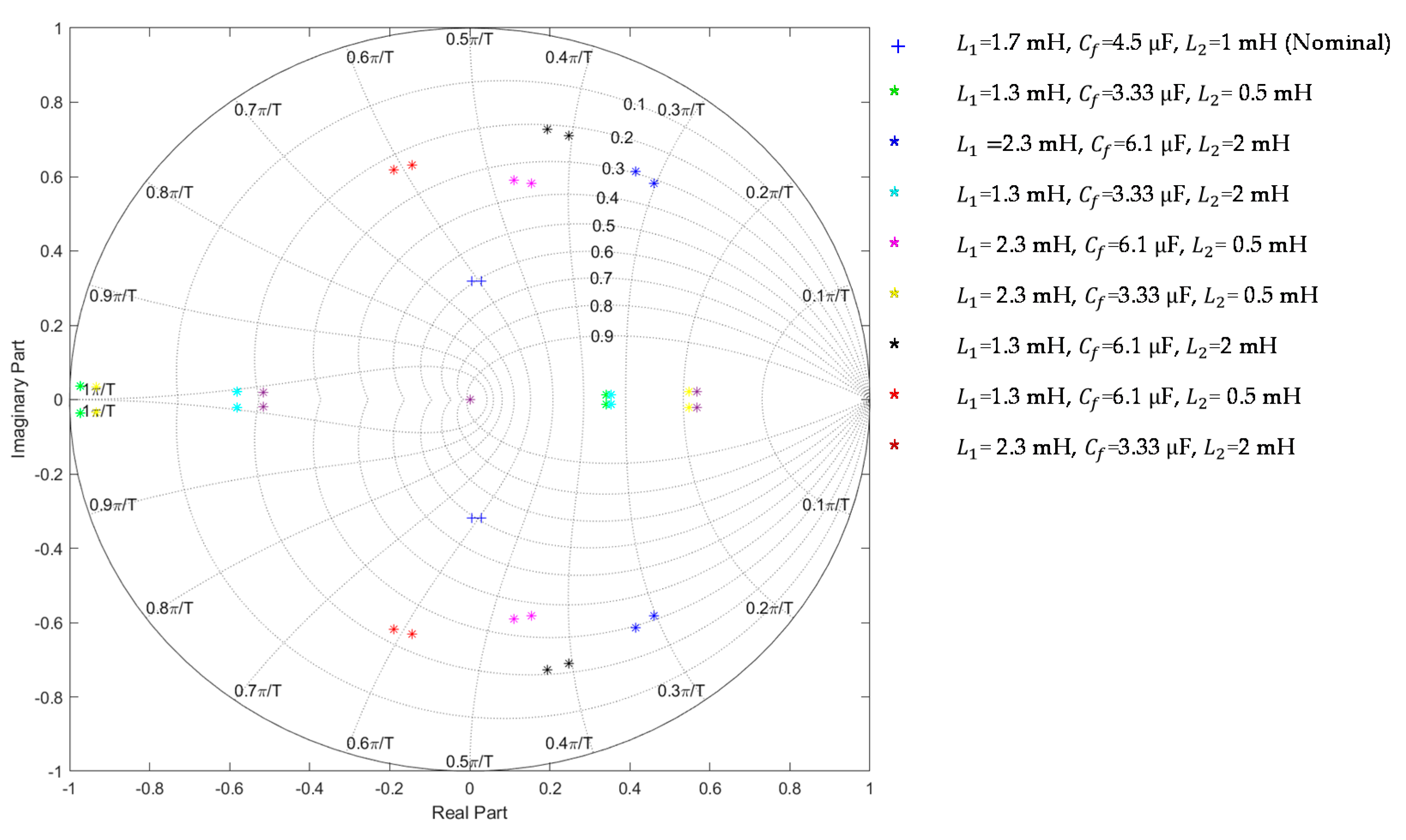
Figure 4 shows the eigenvalues of the proposed MPC scheme under uncertainties of LCL filter parameters.
Figure 5 represents the eigenvalues of the LMI-based current-type full-state observer under uncertainties of LCL filter parameters. In these figures, the uncertainty of parameter values is set by the coefficients
and
. Despite severe LCL filter parameter variations, it is definitively seen that all the eigenvalues of the controller and observer are inside the unit circle. This verifies the robustness of the proposed MPC scheme and observer scheme under the uncertainty of LCL filter parameters.
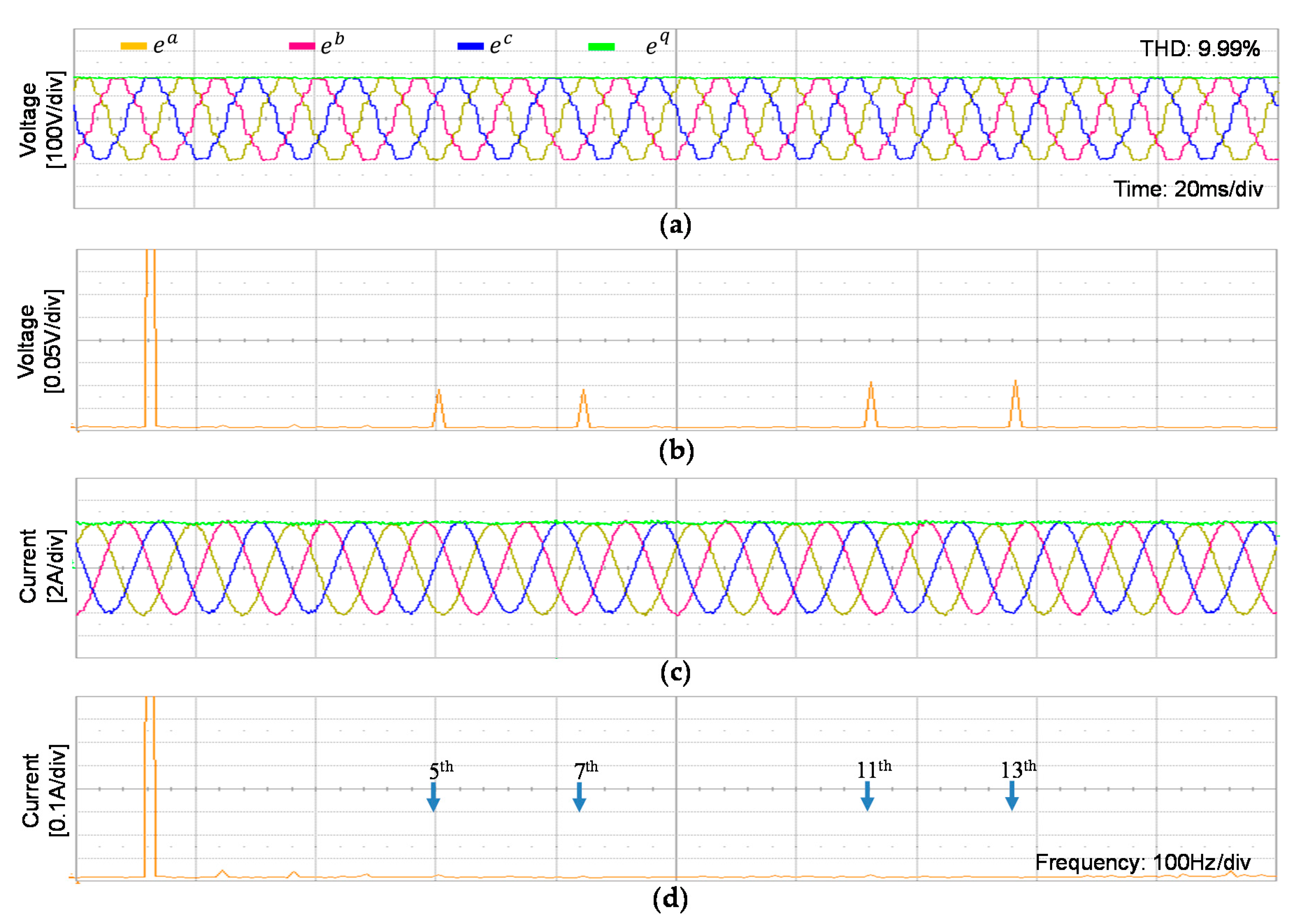
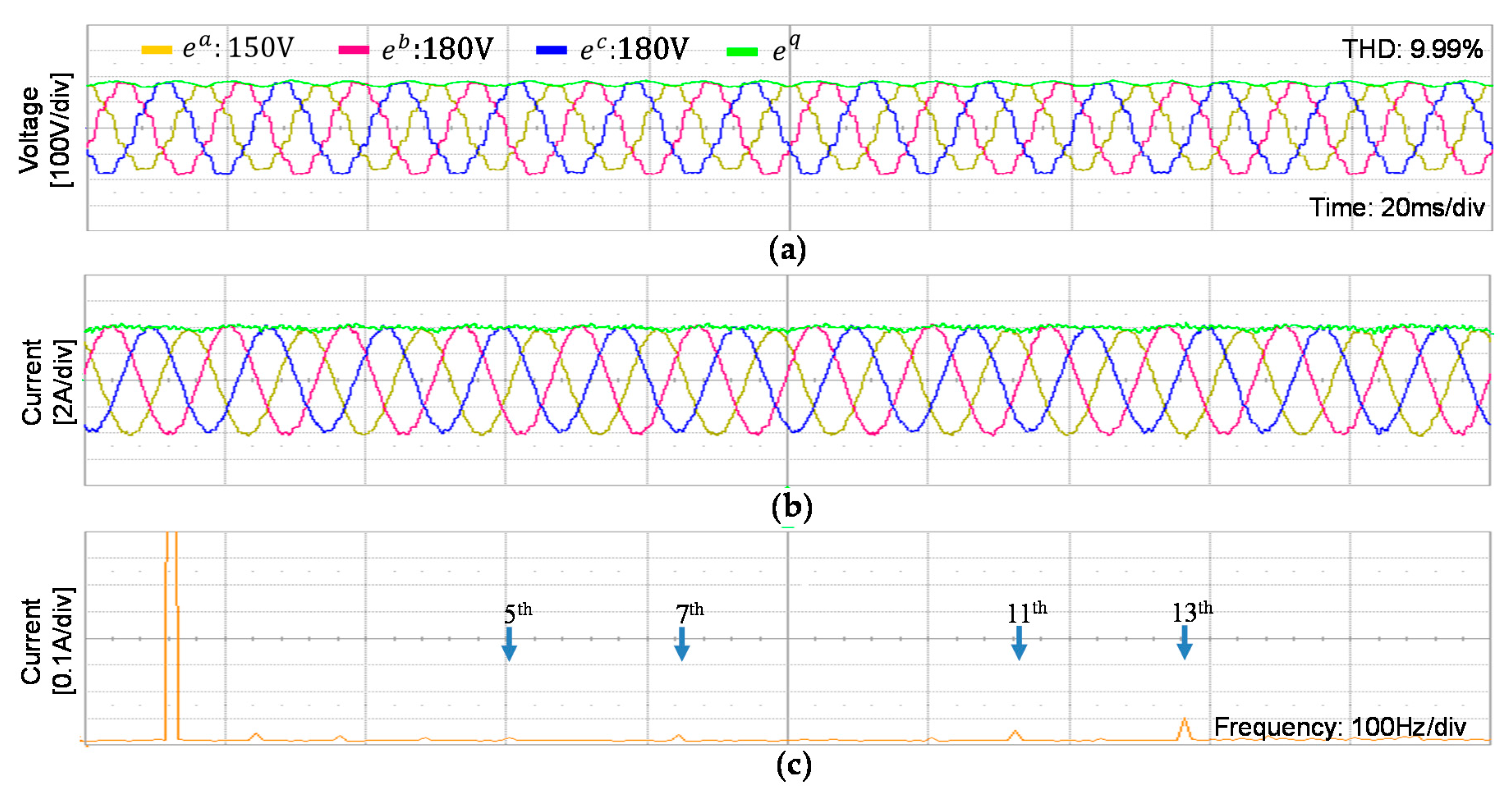
Figure 6 shows the simulation results of the proposed controller under three-phase distorted grid voltages.
Figure 6a represents three-phase distorted grid voltages with the harmonics at the orders of 5th, 7th, 11th, and 13th, with 5% magnitude of the fundamental nominal grid voltages.
Figure 6b shows the result of the fast Fourier transform (FFT) for
a-phase grid voltage, in which the total harmonic distortion (THD) of the grid voltage is 9.99%.
Figure 6c represents the waveforms of three-phase grid currents of the proposed current controller at steady-state, and
Figure 6d presents the FFT result for
a-phase grid current. It is shown clearly that steady-state current control performance is satisfactory, and all the harmonic components caused by distorted grid voltages can be attenuated well. The resultant THD value of phase current is 3.48%, which meets the power quality standard for injected current [
4].
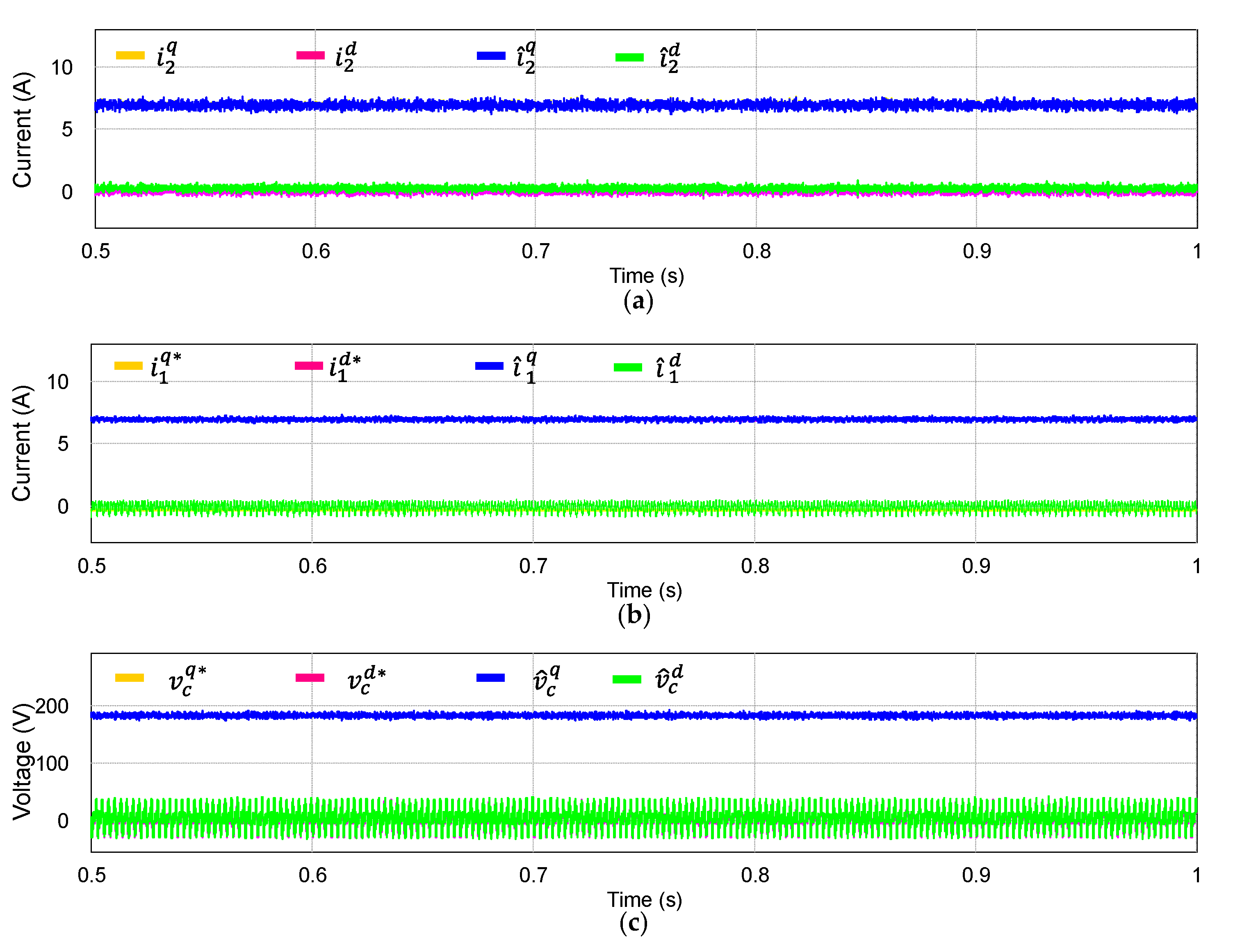
To evaluate the estimation performance of the proposed LMI-based full-state and disturbance observers under distorted grid environment,
Figure 7 shows the simulation results of the estimated states. Even though the LMI-based full-state and disturbance observers are designed in the stationary frame, the estimated states in
Figure 7 are presented at the SRF for comparison purpose with measured variables. In addition, to be compatible with real experimental conditions in which the inverter-side current and capacitor voltage measurements are not available, the reference variables are presented instead of the inverter-side current and capacitor voltage.
Figure 7a presents the waveforms of measured and estimated grid-side currents.
Figure 7b,c present the comparison of the reference and estimated states for inverter-side currents and capacitor voltages, respectively. As is shown in these figures, all the estimated states converge well to their real variables. It is worth mentioning that the outputs of disturbance observer are employed in the reference generation for the MPC in (30)–(31).
To validate the robustness of the proposed current controller,
Figure 8 shows the simulation results of the proposed controller under distorted and imbalanced grid conditions, in which
a-phase grid voltage is reduced to 83.33% of the nominal value, as shown in
Figure 8a.
Figure 8b shows the steady-state performance of the grid-side currents controlled by the proposed scheme, and
Figure 8c represents the FFT result for
a-phase grid current. The current waveforms are quite sinusoidal and balanced without harmonic distortion, which proves the robustness of the proposed scheme under severe grid disturbance.
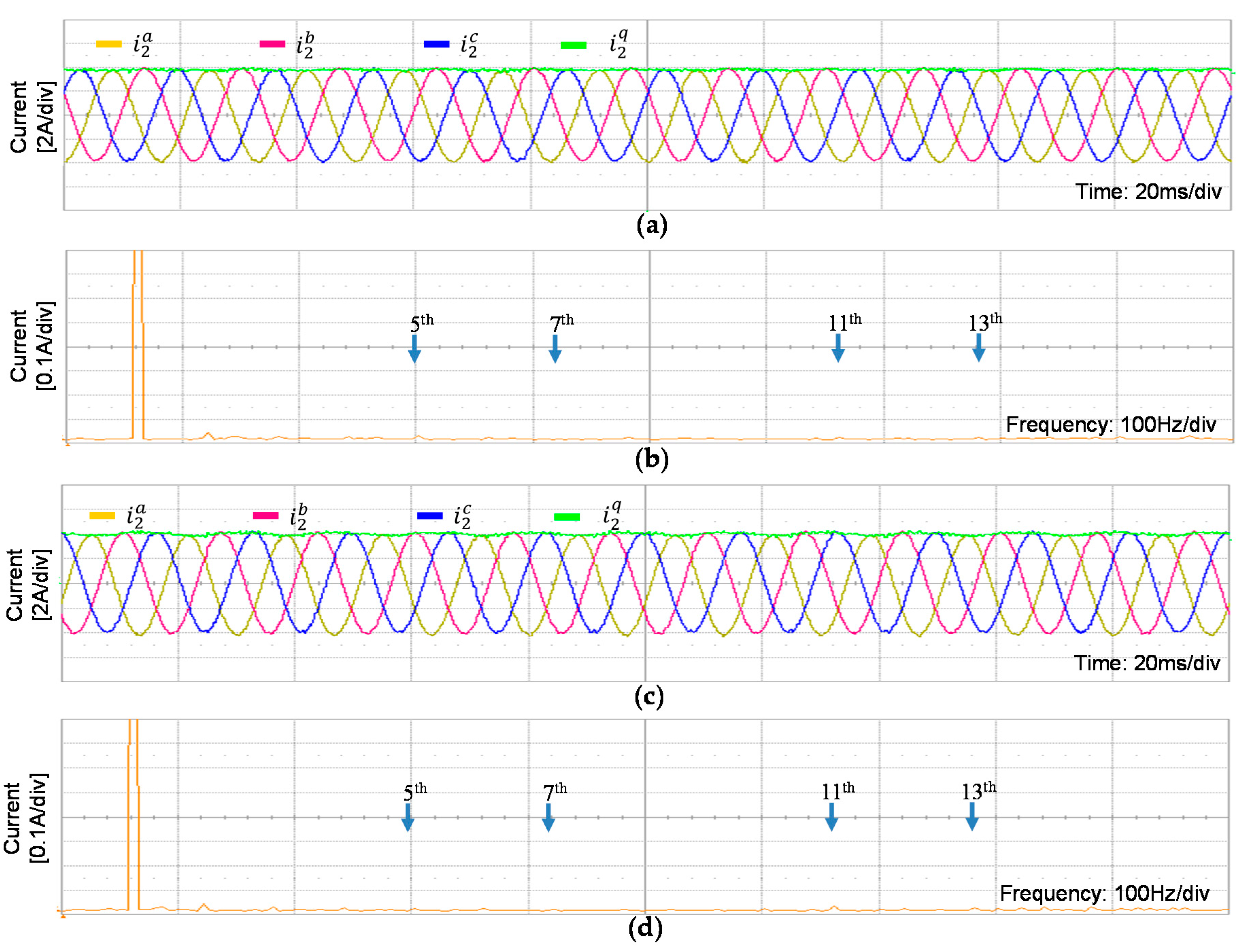
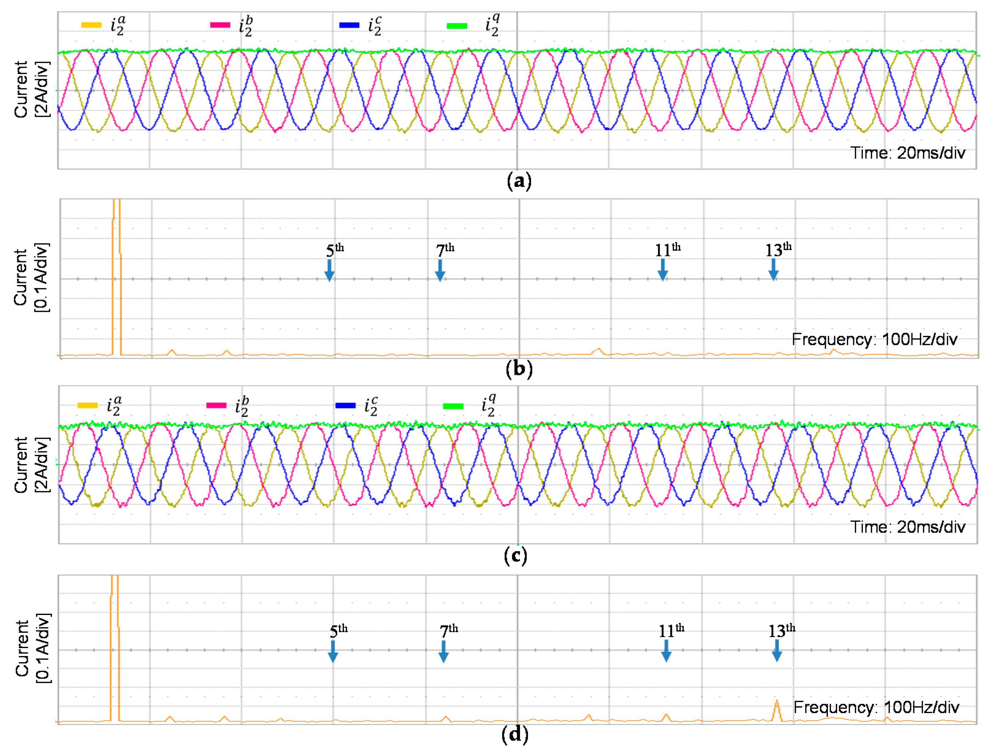
The robustness of the proposed control scheme against the uncertainty in LCL filter parameters is proved under the same grid conditions.
Figure 9a shows the simulation results for three-phase grid-side currents with the proposed control scheme when the filter capacitance
Cf decreases from 4.5 μF to 3 μF under the distorted grid voltages in
Figure 6a.
Figure 9b shows the FFT result of phase-
a current. It is seen that harmonic components caused by the distorted grid are well suppressed and the THD value is only 3.02%.
Figure 10a shows the simulation results for three-phase grid-side currents with the proposed control scheme when the filter capacitance
Cf decreases from 4.5 μF to 3 μF under the distorted and imbalanced grid voltages in
Figure 8a.
Figure 10b shows the FFT result of phase-
a current. The steady-state grid-side currents are sinusoidal and satisfy the grid interconnection criteria. Furthermore, the magnitude of the harmonics is negligible with the THD level of 3.07%. These results clearly demonstrate that the proposed scheme is highly robust in the presence of system parameter uncertainty as well as the grid disturbance such as the distorted voltages and grid voltage imbalance.
To further validate the robustness of the proposed current controller under parameter uncertainty,
Figure 11 shows the simulation results for three-phase grid-side currents with the grid inductance
Lg change from the nominal value to 1 mH. In these simulation tests,
Figure 11a is obtained under only the distorted grid voltages, and
Figure 11b is obtained under distorted and imbalanced grid voltages. Even in this condition, the inverter system still remains stable with high injected current quality. These responses demonstrate the robustness and effectiveness of the proposed MPC scheme under both the internal parametric uncertainties and external grid disturbance, which can contribute to improve the reliability of the GCI systems operating with severe conditions.
Moreover, to verify that the proposed scheme has a frequency-adaptive feature by adopting the MAF to eliminate frequency fluctuations and by updating the filtered grid frequency information in the controller,
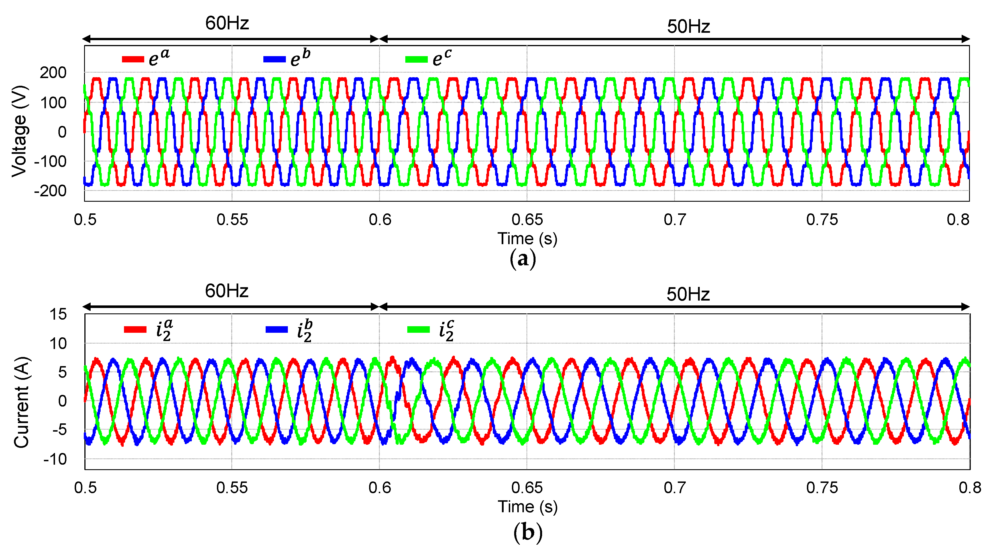
Figure 12 exhibits the transient simulation responses of the proposed MPC scheme under grid frequency variation.
Figure 12a shows three-phase distorted grid voltages with frequency drop from 60 Hz to 50 Hz, and
Figure 12b shows waveforms of three-phase grid currents. As is presented in
Figure 1, the detected grid frequency from the SRF-PLL is fed to the MAF to obtain the filtered frequency which is used in the proposed controller. In spite of frequency change and severely distorted grid voltages, the current waveforms in
Figure 12b show good current quality and lower current overshoot, without noticeable transient periods.
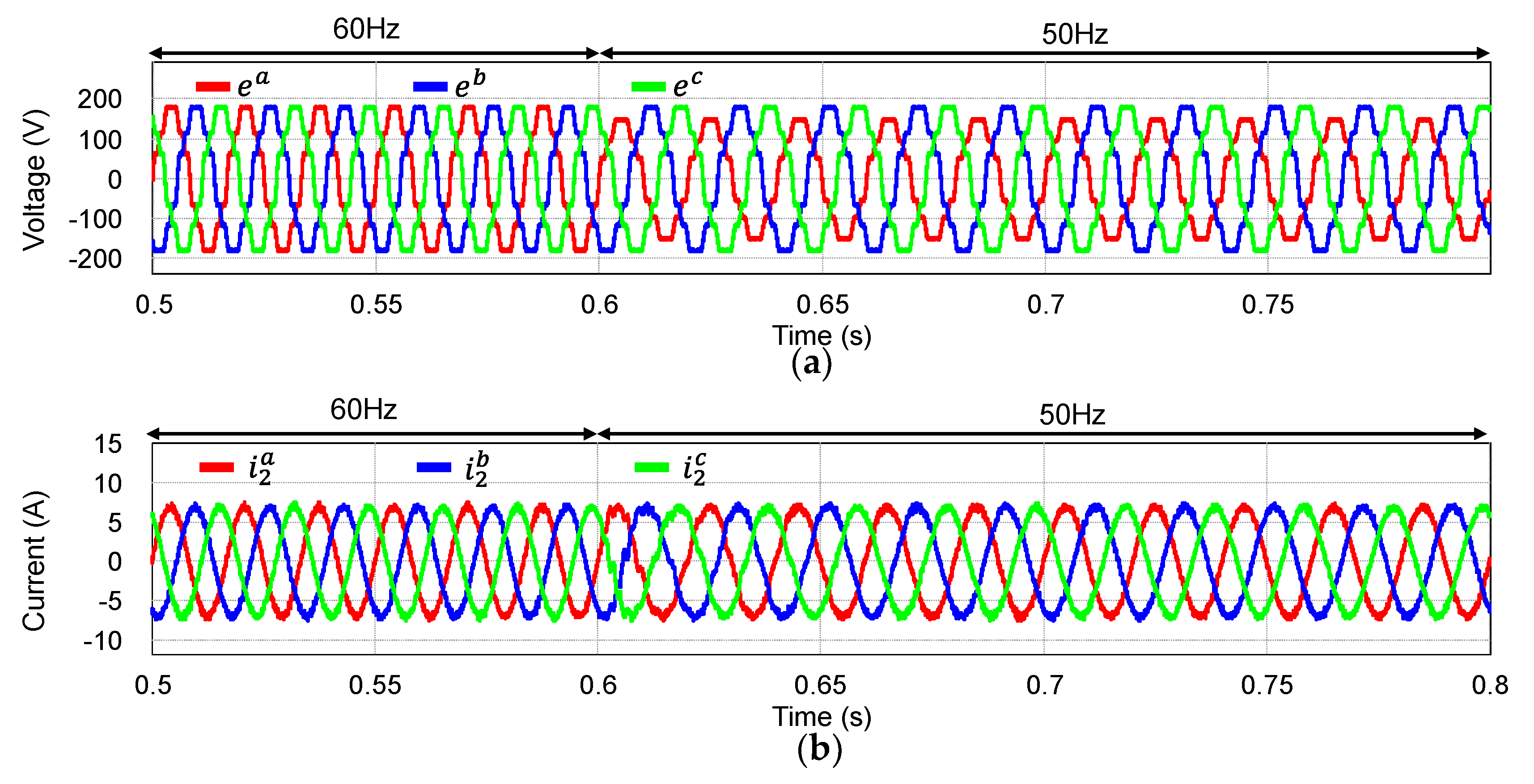
To evaluate the robustness of the proposed scheme,
Figure 13 shows the simulation results of the proposed MPC scheme when the grid voltages have harmonic distortion, imbalance, and frequency change from 60 Hz to 50 Hz at 0.6 s.
Figure 13a shows three-phase grid voltages, and
Figure 13b shows grid current responses in this condition. The current waveforms are still stable and sinusoidal. It is clearly confirmed from these results that the proposed controller stabilizes the inverter system rapidly, even under the frequency variation, and maintains the current quality effectively.
Figure 14 shows the simulation results of the proposed current controller when the current reference has a step change from 4 A to 7 A under distorted grid voltages. The grid-side currents track the reference values instantly, and the current control performance is quite satisfactory with respect to the transient response and steady-state response.
5. Experimental Results
To verify the robustness of the proposed control scheme in a real system, the experimental results are presented by using three-phase 2 kVA prototype GCI system. The configuration of the proposed scheme is represented in
Figure 2, and the system parameters of a GCI are given in
Table 1.
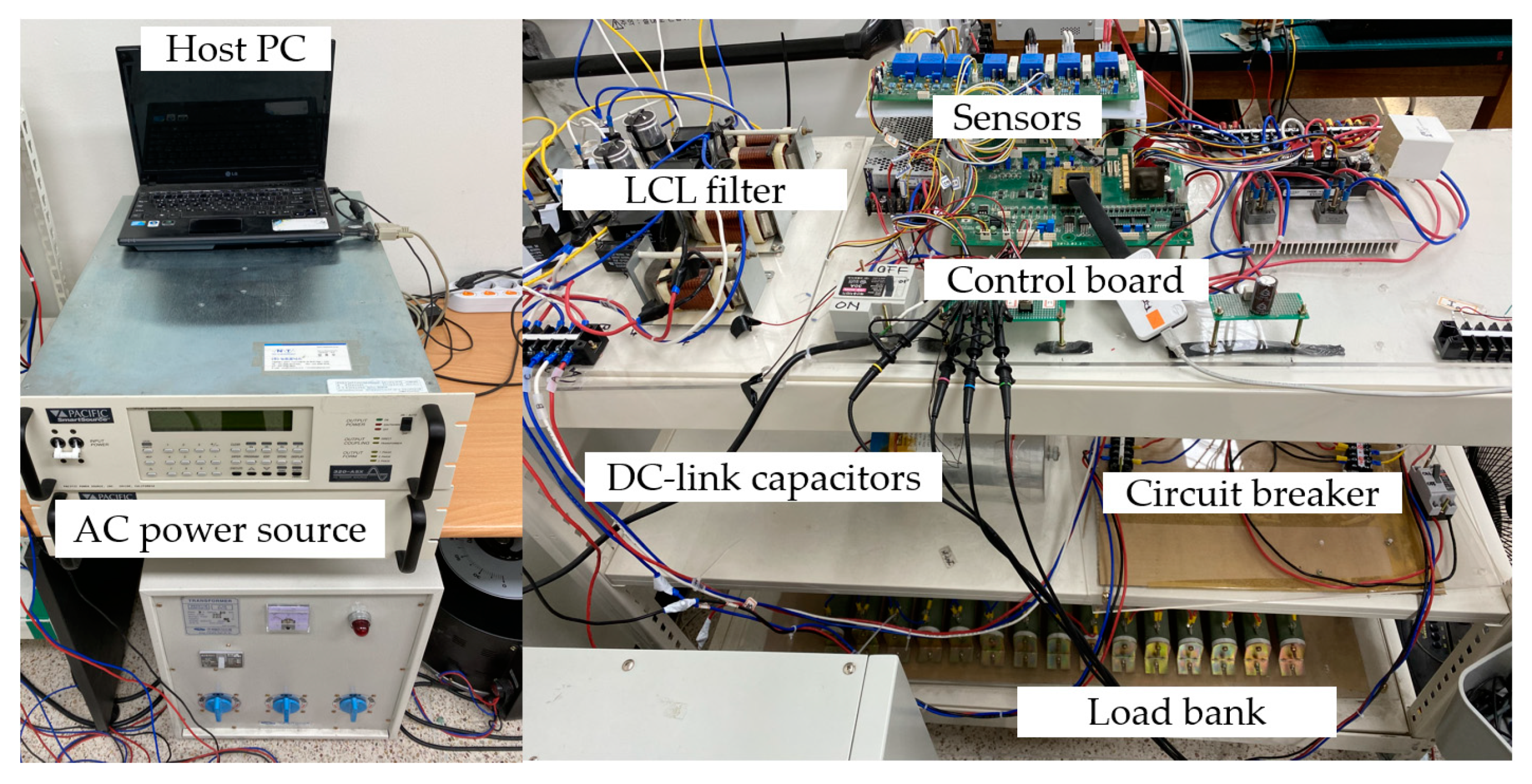
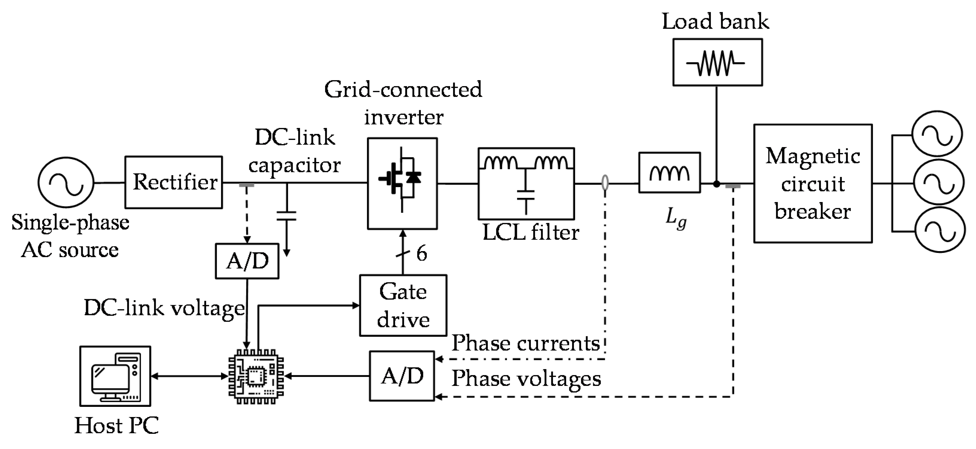
Figure 15 shows the configuration of hardware system, in which the entire system is composed of three-phase GCI connected to the grid through an LCL filter; a magnetic circuit breaker for grid-connecting operations; a DSP controller to realize the proposed control scheme; and a programmable AC power source to generate grid voltage distortion, imbalance, and frequency variation. The control algorithm is implemented on a 32-bit floating-point DSP TM320F28335 with the sampling frequency of 10 kHz.
Figure 16 shows the photograph of the experimental test setup. The execution time of the proposed control scheme on the DSP is represented for each algorithm in
Table 2. The total execution time of the proposed control scheme takes 65% of the sampling period, which is acceptable and can be implemented easily with commercial DSPs.
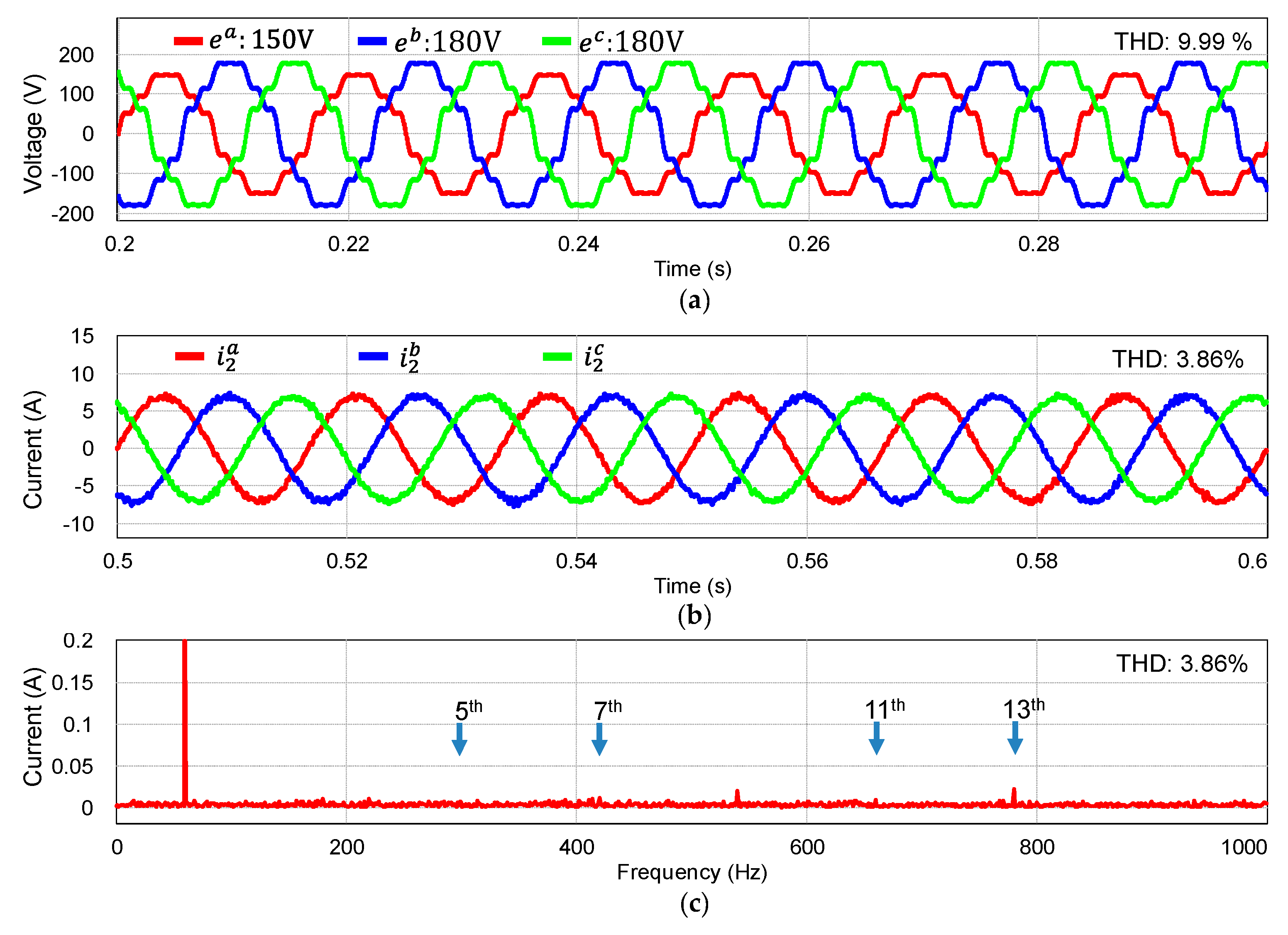
Figure 17 shows the experimental results of the proposed controller under three-phase distorted grid voltages with the same level of harmonic components as the simulation in
Figure 6. The grid reference current is selected to 4 A in the experiment.
Figure 17a,c show three-phase grid voltages and currents in the steady-state condition, respectively. Three-phase grid currents in
Figure 17c coincide well with the simulation results in
Figure 6c.
Figure 17b presents the FFT result of phase-
a grid voltage. The injected grid current quality is represented in
Figure 17d by the FFT results of the
a-phase grid-side current, in which all the distorted harmonics due to main grid are attenuated effectively.
Figure 18 presents the experimental results for the performance of the LMI-based current-type full-state and disturbance observers at the SRF.
Figure 18a–c show the waveforms of measured and estimated grid-side currents, reference and estimated inverter-side currents, and reference and estimated capacitor voltages at the SRF, respectively. Similar to the simulation results in
Figure 7, the system estimated states converge to measured or reference states in steady-state. These results confirm the validity and excellent performance of the LMI-based current-type full-state and disturbance observers.
Figure 19a presents three-phase grid voltages with distorted and imbalanced condition. The reference tracking performance of the grid-side currents controlled by the proposed MPC is shown in
Figure 19b. The FFT spectrum of phase-
a current is shown in
Figure 19c. Even if the 13th harmonic component is slightly increased under this harsh condition in
Figure 19c, the current waveforms are reasonably sinusoidal and balanced.
For next experimental tests, the robustness of the proposed MPC structure against the severe parametric mismatches in LCL filters is evaluated. In
Figure 20, three-phase filter capacitances are varied from 4.5
to 3
and 6
.
Figure 20a depicts the experimental results for three-phase grid-side currents with the proposed control scheme when
Cf decreases to 3
under the same grid condition in
Figure 9.
Figure 20b shows the FFT result of phase-
a current in this condition.
Figure 20c,d show the experimental results of the proposed control scheme when the filter capacitance
Cf increases to 6
with the same grid conditions as
Figure 20a. In the presence of the parametric mismatches, the injected currents of the proposed MPC scheme remains in the balanced sinusoidal waveform with only negligible harmonics, which confirms the strong robustness of the proposed controller.
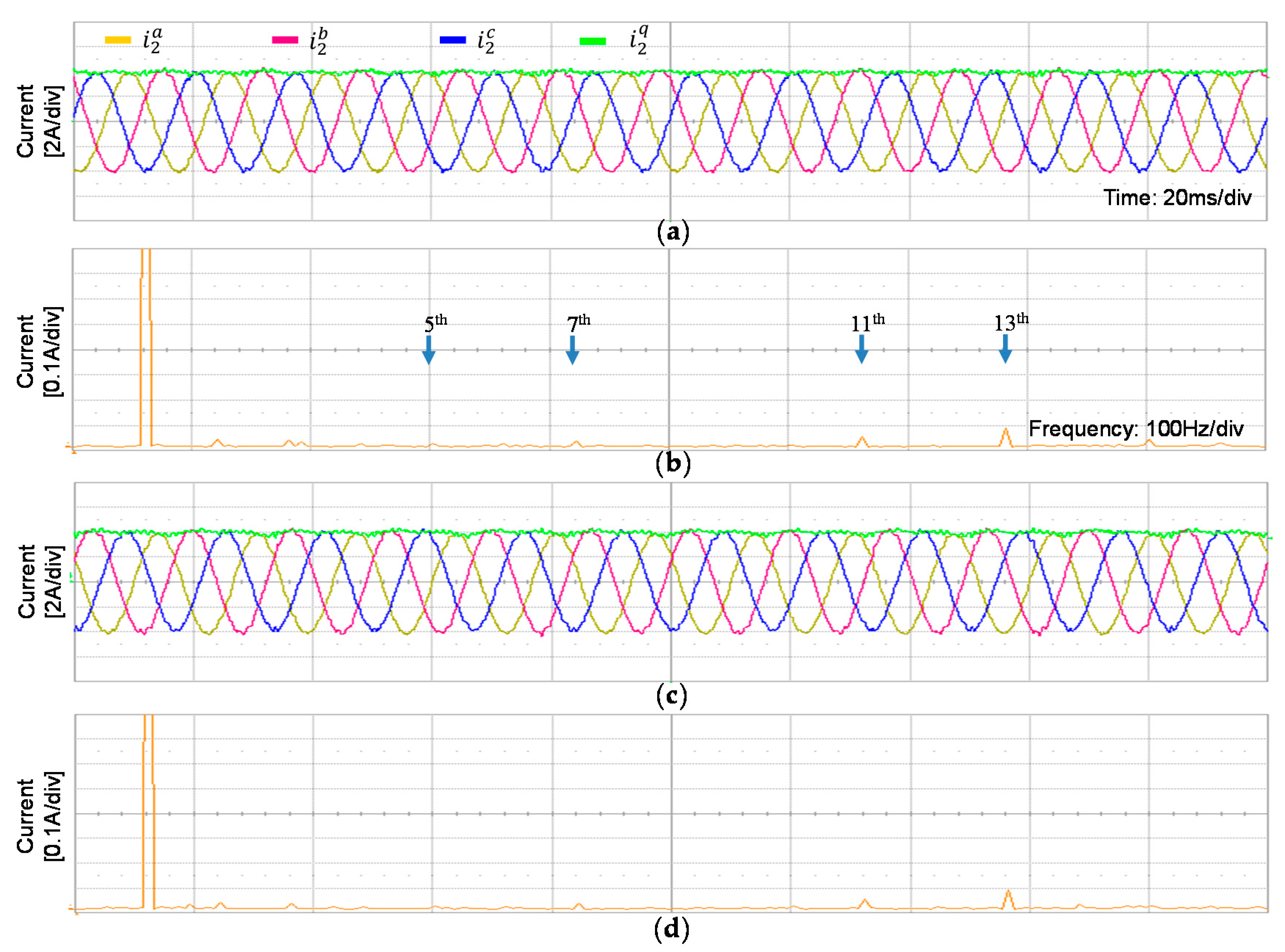
To further evaluate the robustness of the proposed MPC structure against the parametric mismatches under severe grid disturbance,
Figure 21 shows the experimental results when the grid imbalance is added to the experimental conditions in
Figure 20.
Figure 21a,c present the steady-state current waveforms under the LCL filter parameter variations and distorted imbalanced grid voltages with
drop to 83.33% of the nominal value, respectively.
Figure 21b,d show the FFT result of phase-
a current, respectively. The experimental results show the high robustness of the proposed MPC scheme under both the internal parameter uncertainty and severe external disturbance.
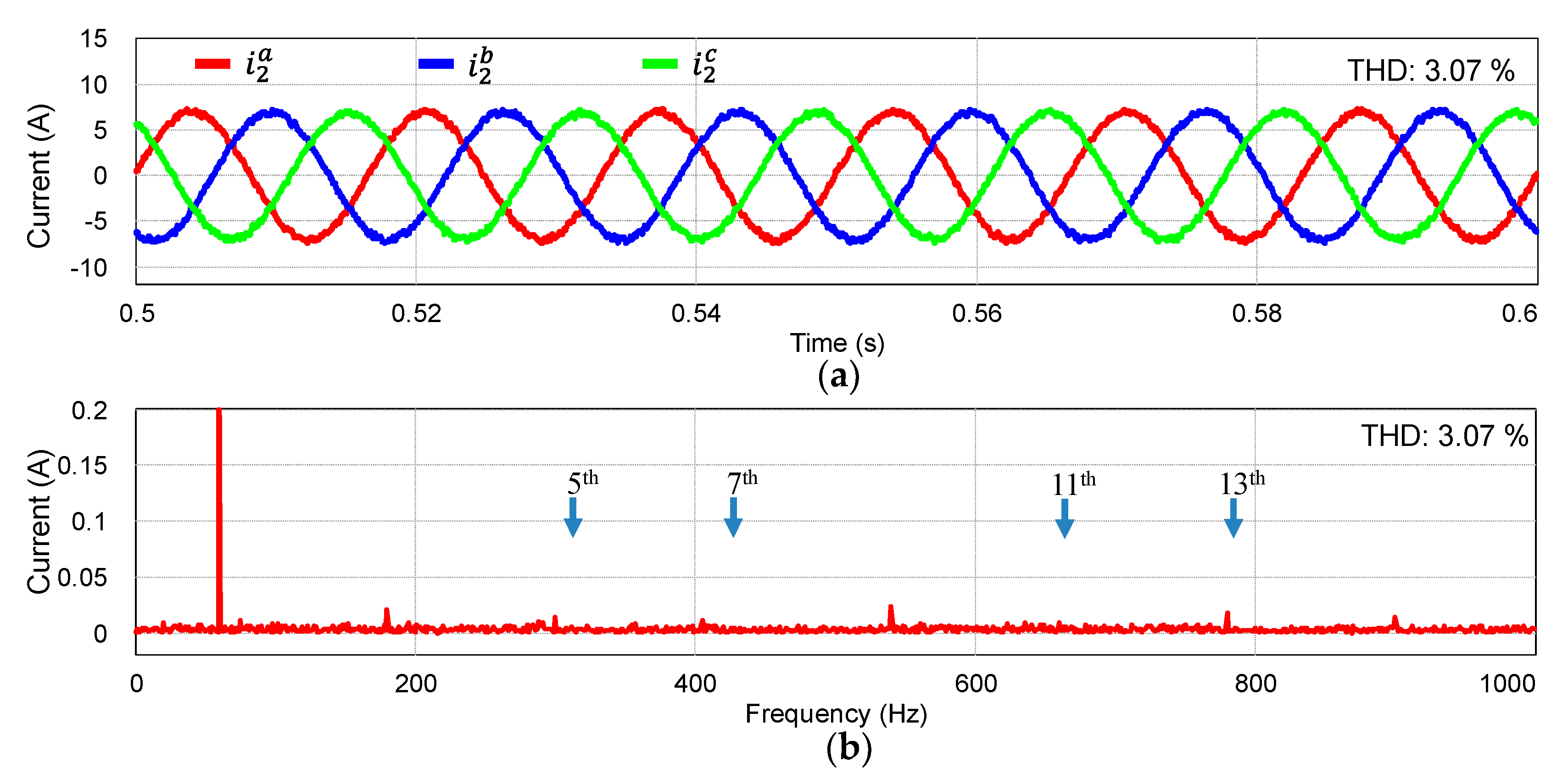
To verify the system performance under weak grid, the grid inductances of 1 mH are added as shown in
Figure 1.
Figure 22a,b depict the grid-injected phase currents and FFT results of phase-
a current under distorted grid voltages, respectively.
Figure 22c,d show the same results when the grid voltages are distorted and imbalanced. High-quality current waveforms in all experimental results prove the robustness of the proposed scheme under non-ideal adverse grid conditions such as imbalanced grid, harmonic distortion, and weak grid.
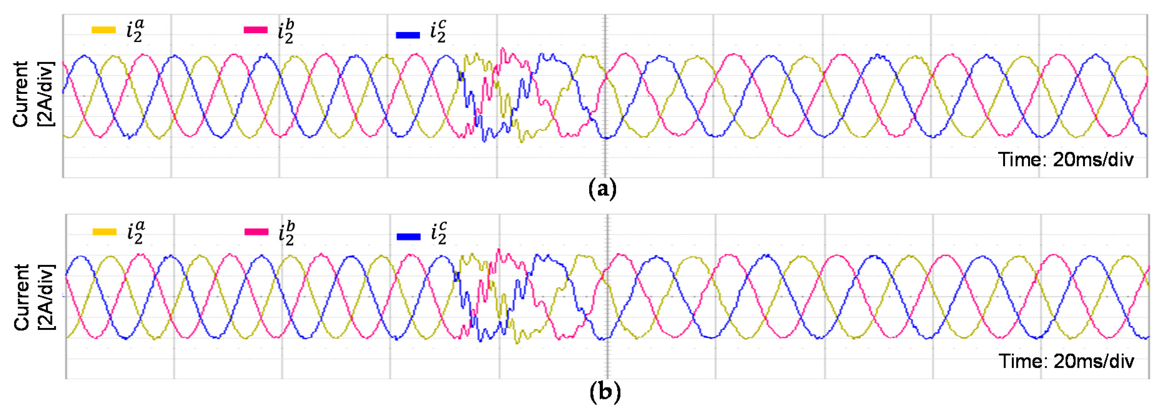
Furthermore,
Figure 23 presents the experimental transient responses of the proposed MPC scheme under grid frequency change from 60 Hz to 50 Hz.
Figure 23a shows three-phase grid-side current responses under the frequency variation and distorted grid voltages.
Figure 23b shows the same results when the grid voltages are distorted and imbalanced. The gird frequency without fluctuation can be acquired by filtering the angular frequency output of the PLL with the MAF in (48). The filtered grid frequency is utilized in (47) to construct the frequency-adaptive distorted harmonic compensators. As a result, the proposed scheme ensures high-quality injected currents even under distorted imbalanced grid voltages and grid frequency variation conditions.
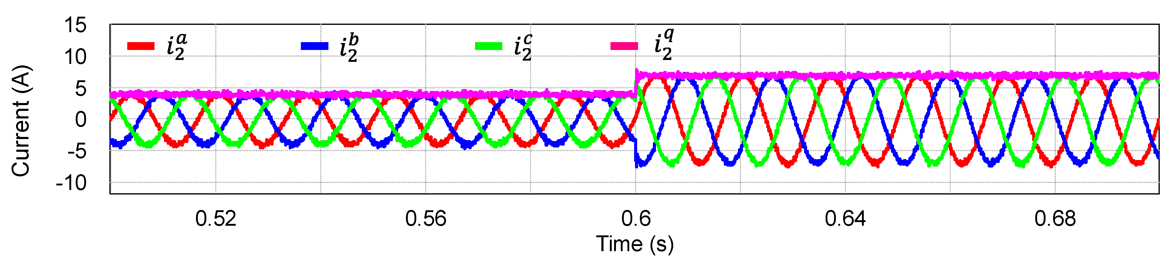
Figure 24 shows the experimental results of three-phase grid currents for the proposed control method under distorted grid voltages when the current reference has a step change from 2 A to 4 A. Similar to the simulation results in
Figure 14, the transient response of the proposed MPC scheme demonstrates the fast reference tracking of the grid currents.
6. Conclusions
To guarantee a system stability and reliable operation of an LCL-filtered GCI under unexpected grid and system uncertainties, an LMI-based MPC has been presented in this paper. Even though the conventional MPC scheme is constructed by a simple concept, it is difficult to determine an optimized weighting matrix of the MPC cost function against parameter discrepancies. The MPC scheme is combined with the LMI-based optimization to overcome such a limitation. To reduce the sensing devices, the system states are estimated by the LMI-based current-type observer. In addition, to improve the reference-tracking performance, the MPC scheme is combined with the disturbance observer. The system stability for the proposed MPC scheme and LMI-based current-type full-state observer is analyzed by investigating the discrete-time closed-loop eigenvalues when the LCL filter parameters vary. The assessment of the stability and current control performance is carried out considering eight vertices of polytopic system model for LCL filter parameters and uncertain grid impedance in the presence of grid disturbance. In comparison with the other studies, the proposed control method ensures high robust control performance under grid voltage imbalance, parameter uncertainty, and frequency variation. Moreover, the proposed approach achieves a robust active damping, even for the grid impedance variation, without the need of considering further damping methods. The proposed control design step is systematic and straightforward. Additionally, the proposed scheme is mainly achieved by offline computing process to obtain the control gains through. Furthermore, unlike the conventional schemes, the proposed controller does not require the augmentation of an integral and 2nd harmonic terms to obtain a good reference tracking performance under grid imbalanced condition, which significantly reduces the controller complexity. To verify the effectiveness of the proposed LMI-based MPC control scheme, the comprehensive simulation and experimental results have been presented by using a prototype three-phase GCI. Test results prove the robustness of the proposed scheme under various adverse conditions with unexpected grid and system uncertainties.


