A Multiview Recognition Method of Predefined Objects for Robot Assembly Using Deep Learning and Its Implementation on an FPGA

Abstract

The process of recognizing manufacturing parts in real time requires fast, accurate, small, and low-power-consumption sensors. Here, we describe a method to extract descriptors from several objects observed from a wide range of angles in a three-dimensional space. These descriptors define the dataset, which allows for the training and further validation of a convolutional neural network. The classification is implemented in reconfigurable hardware in an embedded system with an RGB sensor and the processing unit. The system achieved an accuracy of 96.67% and a speed $2.25\times$ faster than the results reported for state-of-the-art solutions. Our proposal is 655 times faster than implementation on a PC. The presented embedded system meets the criteria of real-time video processing and it is suitable as an enhancement for the hand of a robotic arm in an intelligent manufacturing cell.

1. Introduction

In the field of manufacturing robotics, it is of the highest relevance to count with optical sensors able to provide the system with a sensory mechanism that feeds back the actions of one or more robotic arms that collaborate or interact with a human. Tasks such as welding, machining, painting, or simply clamping and assembly are common in this type of industry. That is why intelligent optical sensing systems are essential for carrying out these tasks. Furthermore, robotics vision allows for automatic learning to achieve fast and accurate object or pattern recognition, which is sometimes a complicated, dangerous, and strenuous task, and humans are usually not involved in the loop. Therefore, these automatic detection mechanisms must be precise when selecting the proper object, which is key to the success of the manufacturing process [1].

In manufacturing cells, it is common for components or objects (e.g., screws, nuts, washers, motors, autoparts, assemblies, and fasteners) to approach the assembly area via conveyors. These objects are usually placed on the worktable of a different assembly robot. These objects are not necessarily approached with the same orientation in each assembly process, and it is even possible that, by some mistake, the part falls and rotates, thus changing the object configuration that was initially planned. It is a highly demanding process to ensure that parts arrive in a specific order and are aligned from the previous stage, so that the robot quickly decides the best way to take them through a deterministic process; this is called the bin-picking problem [2,3]. A robotic vision system must be able to recognize and discriminate parts or objects from any angle and indicate its position to the robot. 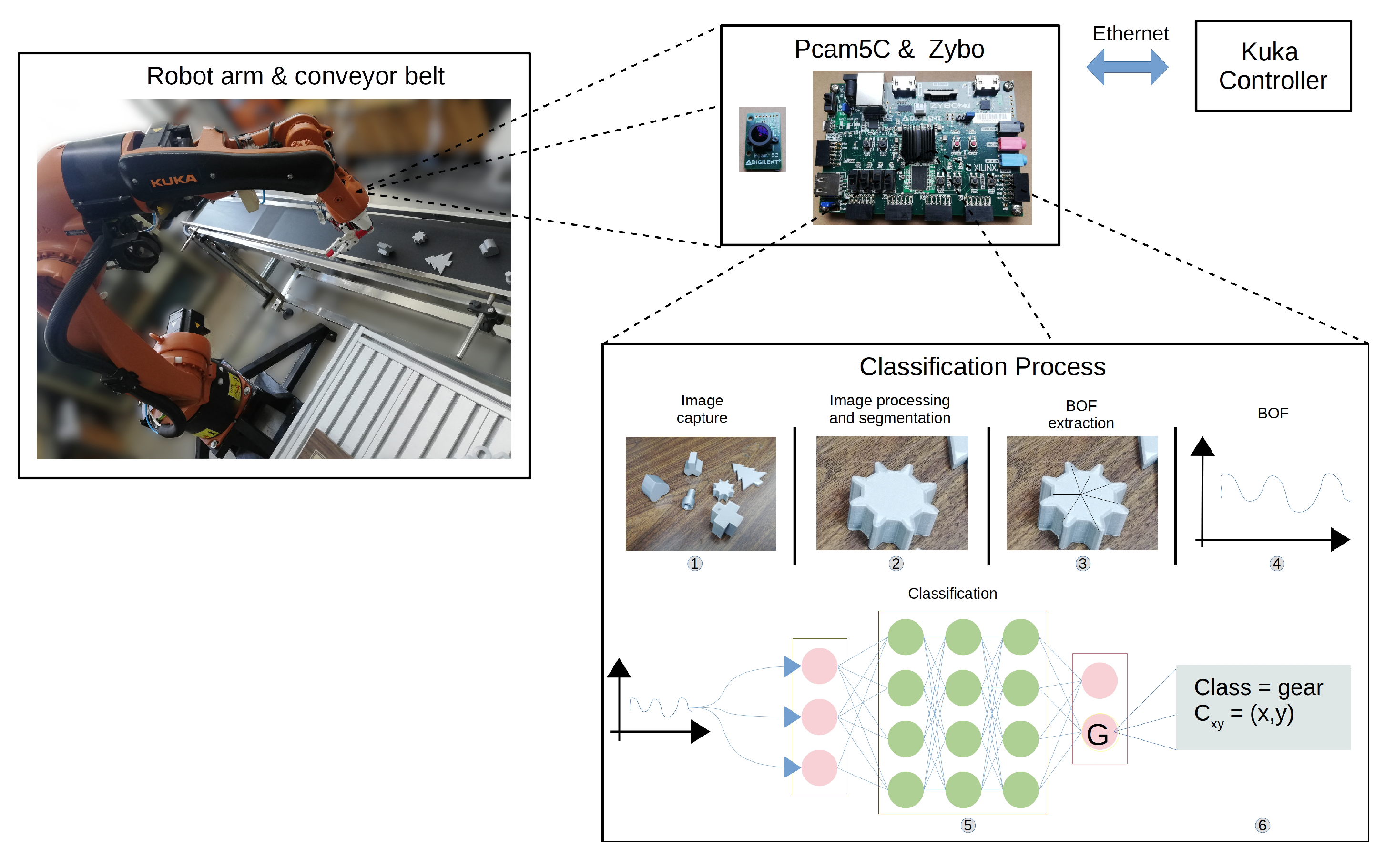These vision systems are either fixed to the manufacturing cell [4] or the last end of the robotic arm [5]. In the former, systems have the advantage that, regardless of the overall weight of the system (camera, communications, and computer), vision systems can be easily installed on tripods or the walls of the cell enclosure. Moreover, power consumption is not critical, although the price is usually high. In the case of vision systems being fixed on the wrist of the robotic arm, advantages appear not only as higher image resolution (closer proximity to the object, higher data quality), but also by offering the possibility of dynamically changing the camera angle. However, in order to not add more weight to the robot, embedded systems able to acquire the image, preprocess it, and make inferences are required. In the context of Industry 4.0, priority is given to low-power, stand-alone, low-cost, multimodal, digitally robust, intercommunicable, and, above all, compact systems [6]. This paper focuses on the second precept, that is, of vision systems attached to a robotic arm.

In contrast to what is commonly found in automatic object recognition in other fields, in intelligent manufacturing, the attributes of the components are perfectly known in advance. Features such as color, geometry, texture, and dimensions are greatly relevant to the system so that it can act on the basis of those descriptions. Hence, it is necessary to use customized procedures since those used in pretrained machine-learning models with a large dataset with hundreds of objects are not functional.

In this contribution, we propose an object recognition method implemented in an FPGA in which tasks such as image capture and preprocessing are automated, and at a further stage, an object classification process is conducted. All these tasks are circumscribed in an embedded system placed on the wrist of a robotic arm. Previous pattern recognition works implemented in FPGA can be divided between those based on feature extraction and those based on artificial neural networks (ANNs). In the former, there is work on the Speed-Up Robust Features (SURF) algorithm [7] and its implementation on FPGA [8], and on Features from Accelerated Segment Test [9] and Binary Robust Independent Elementary Features [10] (FAST + BRIEF) [11]. The ANN approach counts with relevant contributions such as the work described in [12], where it is described as an improved version of YOLOv2 implemented in a ZYNQ FPGA. Convolutional neural networks, CNNs such as VGG16 and MobilenetV2 were implemented in hardware [13] using mixed-precision processors. In [14], several CNN model networks (VGG16, MobilenetV2, MobilenetV3, and ShufflenetV2) were produced in hardware using a hybrid vision processing unit (Hybrid VPU).

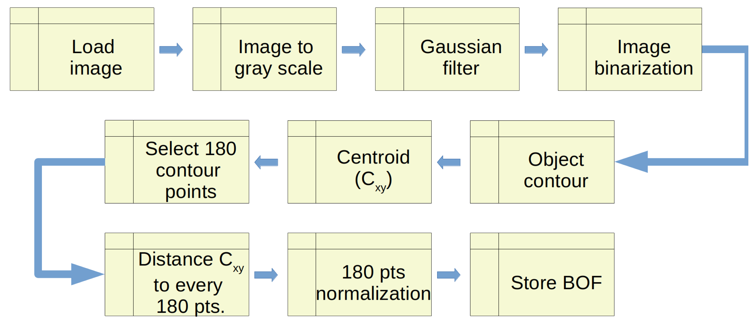
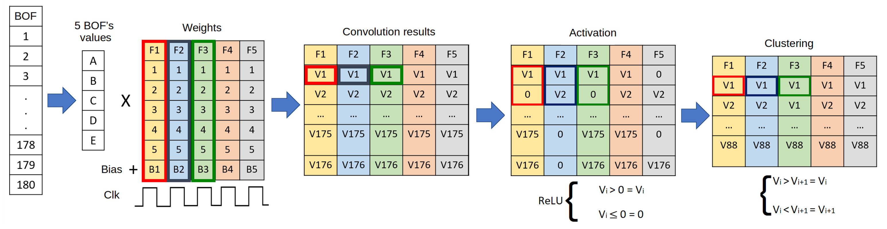
The boundary object function (BOF) [15] descriptor vector, which is a formalism that characterizes an object by extracting some attributes, as detailed in the following sections, demonstrated potential in terms of being invariant to rotation, scale, and displacement, and being able to condense the information coming from a 2D image to a one-dimensional array. In [16], the BOF and a classifier based on the fuzzy ARTMAP neural network were implemented on an FPGA [17] with very favorable results. However, complications are detected when the object angle on the z-axis exceeds 15 degrees. Therefore, object recognition is complicated if the capture angle is different from the considered angle during network training.

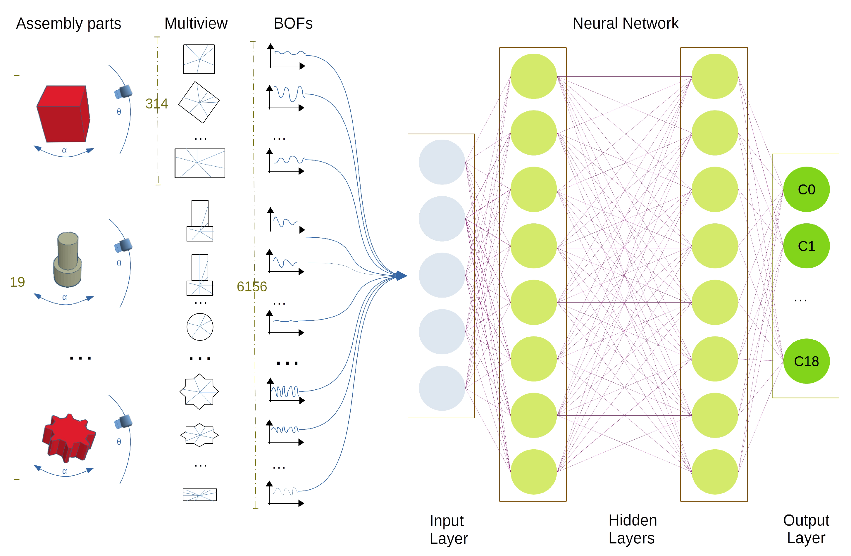
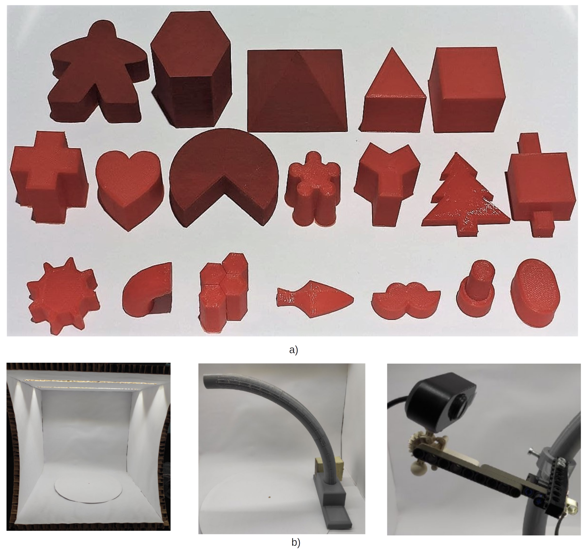
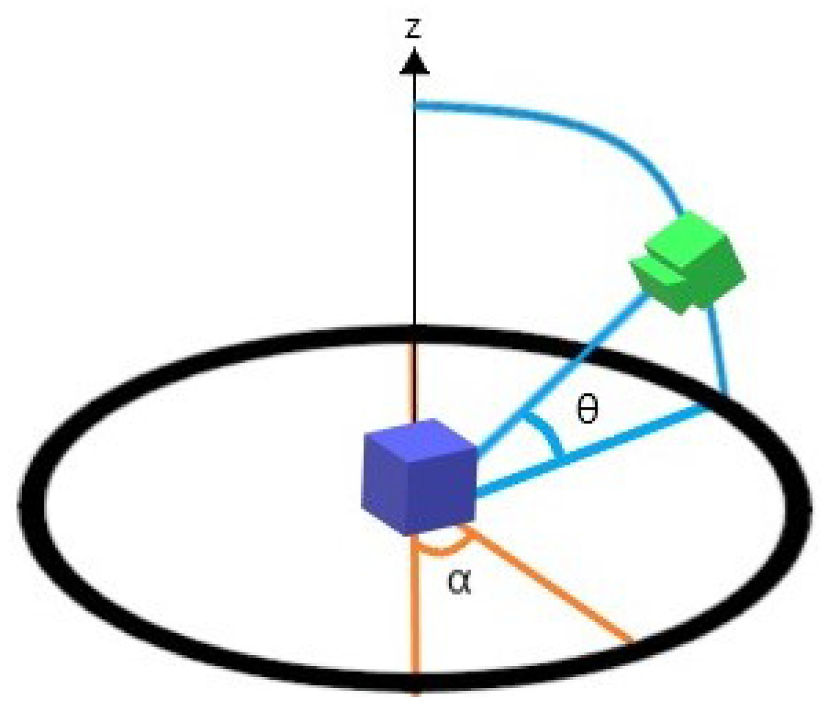
We constructed our dataset by joining the descriptors of all objects. First, a family of BOF vectors linked to a given object was obtained by systematically rotating the camera plane around a surrounding sphere centered on the object. Then, a BOF was obtained from each rotation angle, and the family of BOFs could be tuned by setting the list of rotation angles. Lastly, all objects of interest were characterized in the same form, and the family of BOFs associated with each constituted the complete dataset, as shown in Figure 1.

Although CNNs were originally designed for digital image processing, they were successfully applied in several other contexts. Applications in other areas include, for example, genomic data processing [18], text classification [19], and sentiment analysis [20].

In our contribution, the challenge was to find a CNN model that could classify BOF vector families of different objects.

Table 1. Image size for every model compared with BOF vector size.

Model	LeNet-5	AlexNet	VGG-16	GoogLeNet	ResNet-50(v1)	BOF and CNN
Size (pixels)	32 × 32	227 × 227	231 × 231	224 × 224	224 × 224	N/A
Total (bytes)	1024	51,529	53,361	50,176	50,176	180 × (nbytes fixed point)

shows the pixel input dimensions for the most common CNN models and the BOF and CNN combination introduced in this work. The input dimensions for this case were defined as a 180 × (nbytes fixed point) since the BOF consisted of 180 values, that is, 180 angles of rotation represented as a fixed point.

As stated earlier, in this contribution, we describe a method to classify objects using their BOF vector family as features. The external label or class is given by the object type, such as screws or gears. A deep learning neural network then approximates a function between BOF family vector and object class. The main contributions are:

• we designed a manufacturing part recognition method capable of classifying multiple part views from their unique descriptors (BOF);
• we designed a CNN from an existing model, but instead of directly using images, we trained the network with the unique descriptors of each part view; and
• we implemented a CNN model on a field-programmable gate array (FPGA).

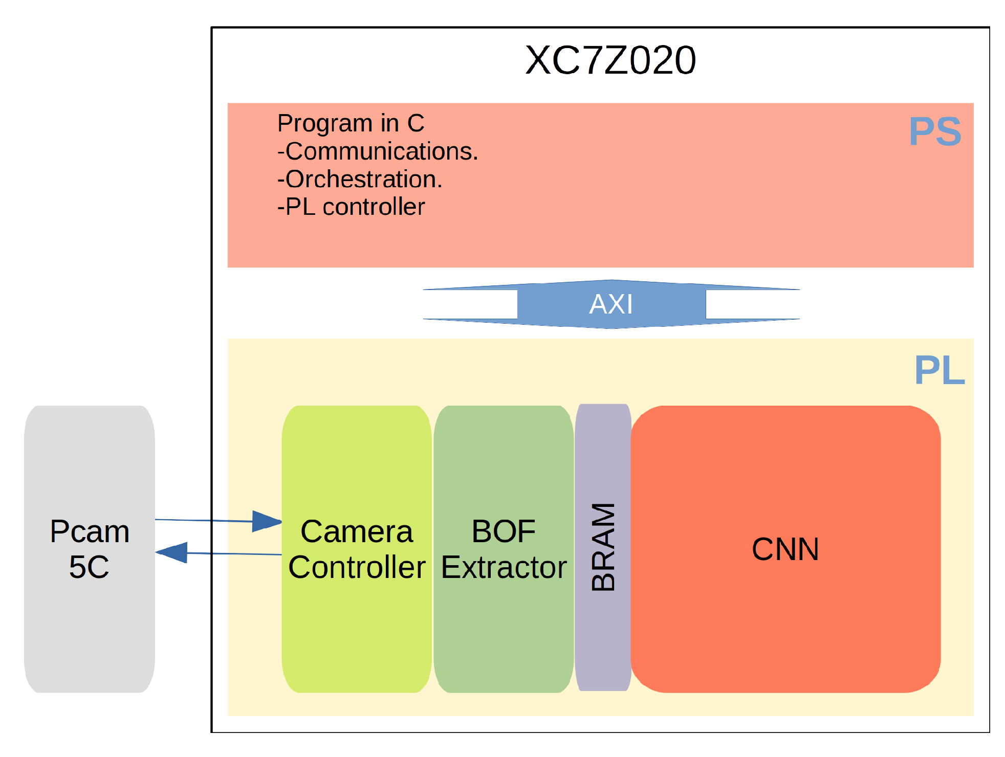
In this contribution, the hypothesis we aimed to prove is that objects of interest in automatic manufacturing can be recognized by their BOF description instead of relying on their images. Since BOFs are vectors representing objects, and BOFs have lower dimensions than images do, we aimed to successfully train a CNN as a classifier on the basis of BOFs. At the same time and equally relevant, we wanted to verify whether training based on BOFs is faster. The third relevant aspect we investigate is the method’s speed gain when implemented in an FPGA (Figure 2).

Related works [13,14] relied on an image detection algorithm based on a CNN. However, the size of the networks is described by its more than 2 million parameters (Mobilenet V2), which consumes 279,000 LUTs and 3600 DSP, and 146,000 LUTs and 212 DSP, respectively. Instead, our model consumes only 31,336 LUTs and 116 DSP. As an additional advantage of our proposal, as is shown in the next sections, it is faster.

The rest of this study is organized as follows. Section 2 describes the entire process of building the dataset, the design of the CNN, and its implementation on the FPGA. Section 3 shows the nature of the data and is divided into two sections: results of the CNN implemented in Python to ensure network efficiency and the results of FPGA implementation. Section 4 shows the main results by comparing the results achieved by our contribution with those of similar works. Lastly, Section 5 presents some concluding remarks.

The method presented in this paper aims to answer these questions.

2. Materials and Methods

The methodology supporting this work consists of the following stages:

• Select a set of manufacturing parts and print them with additive manufacturing.
• Obtain images of each object varying the rotation angle on the z axis and the azimuthal angle.
• Extract the BOF descriptive vector from each image.
• Create a dataset with data from the previous point.
• Select a suitable CNN and adjust its parameters, including its architecture, to achieve the best performance and minimize the loss.
• Implement the CNN architecture on the FPGA.
• Compare the results.

2.1. BOF Extraction and Dataset Conformation

We designed 19 assembly objects in a 3D rendering tool. Elements were printed using a 3D printer, and we conducted the training and testing phases over those objects. Some of those objects are shown in Figure 3a.

We built a small photographic studio (35 × 35 × 31 [cm]) to take pictures of objects at different angles (Figure 3b). It could rotate an object $\alpha$ degrees every $\Delta \alpha$ through a stepper motor with which the rotation is parameterized. Moreover, the $\theta$ camera tilt angle could be adjusted by means of a 90-degree arc-shaped bracket graduated every 5 degrees. Thus, manual setting $\Delta \theta$ was also parameterizable.

The dataset (“3DBOFD”, 3D BOF Dataset) was generated as follows:

• Set $\alpha$ and $\theta$ to initial position (see Figure 4).
• Obtain object image.
• Calculate the BOF. Figure 5 shows the process of extracting a vector BOF from an object [15]. Reduce the dimension of this vector by taking the contour points that are separated by 2 degrees. The BOF vector’s dimensions are 180 × 1.
• Rotate the object $\Delta \alpha$ degrees on the z axis to complete 360 degrees and repeat Steps 2 and 3.
• Tilt the camera $\Delta \theta$ and repeat Steps 2–4 until completion from 0 to 90 degrees.

2.2. CNN Model

A neural network is a universal classifier. In our context, this property is translated as the capability of finding a function that relates to two sets. In our particular case, those sets were, on the one hand, the attributes describing an object, and on the other hand, the type or class of that object. Convolutional neural networks perform an iterative transformation of vectors from the initial attribute space to new spaces. The core idea is that several attributes are extracted in each stage, and, at the last stage in this class of neural networks, classification is performed in a new feature space via a classifier that may be a neural network.

As a first approach to model the convolutional neural network, we used the LeNet-5 network [21] due to its small size (number of layers, kernel size, and number of parameters).

Table 2. LeNet-5 CNN model.

Layer	Size
Input	1@32 × 32
Convolution	6@28 × 8
Average pooling	6@14 × 14
Convolution	16@10 × 10
Average pooling	16@5 × 5
Dense	120
Dense	84
Dense	10

shows LeNet-5 architecture. Its original purpose was to recognize handwritten or printed digits. Therefore, input images must be rescaled to 32 × 32 pixels.

Since the dimensions of the BOF (180 × 1) were incompatible with the 32 × 32 pixel input of LeNet-5, a modification of the layers was proposed as follows (see

Table 3. First CNN model adaptation.

Layer	Conv1	Max-Pooling1	Conv2	Max-Pooling2
Original size	5 × 5	2 × 2	5 × 5	2 × 2
Adapted size	1 × 5	1 × 2	1 × 5	1 × 2

).

It was initially determined that $\Delta \theta ={10}^{\circ }$ and $\Delta \alpha ={10}^{\circ }$. Thus, 360 images were generated for each object. However, when $\theta =0^{\circ }$, the obtained perspective was very similar between some objects for most $\alpha$. The latter was because the arrangement with which the images of the objects in the study were taken sharply coincided. Each object was placed with its face (cross, semicircle, or triangle) along the z axis. However, the other face of the object (the height) was parallel to the angle when theta equals zero, making it look like a rectangular outline in all cases. In consequence, all images of the objects were discarded when $\theta =0$, resulting in 324 images per object and 6156 images in total.

We implemented the LeNet-5 network (see Table 2) in Python through Keras considering the input vector size imposed by the network design. In order to obtain the best performance of the network, several regularizations and optimization techniques were performed.

Two new convolutional layers of 12 and 24 filters with 1 × 5 kernels were added. In addition, the number of filters in the first convolutional layer was reduced to 5, and 8 in the second convolutional layer. The first convolutional layer was also reduced to 90 neurons. The CNN model implemented in the FPGA is shown in

Table 4. Parameters of final CNN model.

Layer	Out Dimension	Number of Parameters
Conv1	(176, 5)	30
Max_pooling1	(88, 5)	0
Conv2	(84, 8)	208
Max_pooling2	(42, 8)	0
Conv3	(38, 12)	492
Max_pooling3	(19, 12)	0
Conv4	(15, 25)	1525
Max_pooling4	(7, 25)	0
Dense1	(1, 90)	15,840
Dense2	(1, 84)	7644
Dense2	(1, 19)	1615

.

2.3. CNN FPGA Implementation

BOF and CNN implementation was performed on a Zybo Z7-20 Digilent board with the Zynq-7000 SoC (XC7Z020-1CLG400C) from Xilinx. In addition, we used Digilent’s Pcam 5C module for image capture, which is based on Omnivision’s OV5640 RGB sensor.

Figure 6 shows the architecture of the BOF implementation on the FPGA.

2.3.1. Fixed-Point Determination

We opted for a fixed-point representation for BOF and CNN implementation, which carries a cost in accuracy since it is necessary to round or truncate the result at the end of an operation. In addition, this rounding truncation produces a quantization error [22]. Therefore, we tested with different fixed-point formats to establish the best representation in BOF and CNN implementation on the FPGA. As our reference is the implementation of the BOF and CNN on a CPU using Python and Keras, it was necessary to compare each layer of the CNN implemented in Python with the implementation in VHDL. With the use of the fxpmath library [23], fixed-point numbers were presented, and the error was estimated.

For representation in each stage (BOF, CNN convolutional layers, CNN dense layer, and CNN classification layer), classifications were performed with 100 samples with different fixed-point resolutions.

Table 5. Accuracy of n-bit fixed points per stage.

Stage	# of Bits → Accuracy
BOF	7 → 92.0% | 9 → 96.0% | 11 → 98.0%
Conv. and Fully connected layers	9 → 40% | 16 → 96%
Classif. layer	32 → 97%

shows the accuracy percentages by iterating with different numbers of bits for each stage. For instance, the accuracy of 7 bits for BOF representations was 92%, but if we use 9 bits, accuracy improved to 96%. The same case was observed with convolutional layers where, using only 9 bits, accuracy was barely 40%; instead, using 16 bits, accuracy improved to 96%. Results improved by adding more bits; however, resources used in the FPGA then considerably increase. Thus, for the BOF extraction stage, 9 bits were used; for the convolutional and Dense layers of the CNN, 16 bits were used; and for the classification layer, it was necessary to use up to 32 bits.

Table 6. Number of bits for every fixed point part in every stage.

Stage/# of Bits	Sign	Integer	Decimal
BOF	1	1	7
Conv. layers	1	3	12
Fully C. layers	1	7	8
Classif. layer	-	24	8

shows the number of bits for each part of the fixed-point representation and their set for each process stage.

2.3.2. BOF Stage Implementation

The authors in [16] described how BOF elements are extracted. First, these values are stored in a BRAM. Then, 5 by 5 data are taken to introduce them to the input of the first layer of the CNN, which has a 1 × 5 kernel.

2.3.3. Convolutional Layer Implementation

Each convolutional layer comprises the following stages: convolution, activation, clustering, and memory storage. In the first stage, convolution is performed with incoming data. In the second stage, the chosen activation function is applied; in the third stage, the most representative values are grouped according to the selected strategy; and in the fourth stage, resulting values are stored.

Table 7. Parameters for convolutional and max-pooling stages.

Stage	Kernel	Stride	Padding	Activation
Conv.	1 × 5	1	None	ReLU
Max pooling	1 × 2	2	None	-

shows the parameters for the convolutional and max-pooling stages.

This layer consisted of five filters (25 in total) multiplied by the five values of the input (BOF) and summed. The corresponding bias was added at the end of the stage (Figure 7). Subsequently, values that passed to the clustering stage were determined in the activation stage. These consisted of 5 data. Meanwhile, 5 new data were received from the BRAM, where the BOF was stored, and the previous procedure was repeated. Lastly, a 1 × 2 filter was applied in the max pooling stage with a stride of 2. The output dimension was half of the input dimension.

Due to the accumulated latency, data were stored in a buffer at the output of the first, second, and third convolutional layers. However, this buffer was no longer necessary in the fourth convolutional layer as the data were passed directly to the dense layer.

2.3.4. Dense Layer Implementation

Dense layers have three stages: the sum of products, bias, and activation. In total, 175 values were received from the fourth convolutional layer for the first dense layer. In the sum of products and bias stage, 25 operations were performed per cycle to reduce the use of FPGA resources. Then, the remaining 150 values were consecutively operated on until the end. At the output of this stage, 90 values were processed in the activation stage through a ReLU function. At the output, there was a buffer that passed the data to the next layer. In total, 90 data are received in the second layer, and 84 were delivered and buffered.

The third dense layer was similar to the previous layers; however, the applied activation function was the softmax function. Again, due to the complexity of implementing the exponential function in VHDL, HLS was used for its implementation.

In particular, we relied on the hls_math.h library, which contains the exponential function. We converted fixed-point data from the previous step into a floating point because using a fixed point in exp HLS function caused synchronization issues, so the ap_fixed.h library was called. Once the value of the softmax function had been obtained, it was necessary to return the data to the 32-bit fixed-point format. We used this particular length because the exponential output was expected to be in the range from hundreds of millions to values close to zero.

Lastly, the classification layer determined the class associated with the input BOF. The procedure for this final stage was as follows:

• All exponentials of the previous layer are stored and added up.
• Each exponential is divided by the total of the exponentials, and the one with the highest value is stored.
• The class index with the highest value is the class with the highest classification probability.

2.3.5. FPGA Processing System

BOF extraction and the CNN use the programmable logic of the XC7Z020; however, the processing system performs the following tasks:

• Communication with the Kuka KRC5 robot controller through the MQTT protocol.
• The PS receives control commands and configuration from both the board components, and the acquisition and sorting process implemented in the PL.
• The PS also sends status data and can send an image or the data of the found object, such as the centroid class to which it belongs and even the classification percentage of all classes. Thus, the robot can grasp the part.

3. Results

This section first shows the main results of the CNN model implemented in Python and Keras. Then, we present obtained results from the implementation of the CNN in the FPGA.

3.1. Results for CNN Model Selection

Several tests were performed to obtain the best CNN architecture model to solve the task described in the previous section. First, the dataset was split and randomly sorted. For the training stage, 60% (3694) was selected, 20% (1231) for validation, and 20% (1231) for testing the model.

In order to achieve a robust model, the whole process was performed three times. The following four stages describe the flow of the process: (1) training the network and conducting a classification to validate performance; (2) calculating several performance metrics (error, loss, and accuracy); (3) adjusting the number of layers, size, and parameters; (4) redesigning in order to improve the considered metrics.

Table 8. Accuracy and loss for modified CNN model.

CNN Model	Loss or Acc.	Training	Validation	Test
LeNet-5	Loss	0.0111	0.1657	0.1361
	Accuracy	0.9996	0.9594	0.9594
1st version	Loss	0.1731	0.1277	0.1407
	Accuracy	0.9409	0.9602	0.9521
Last version	Loss	0.312	0.0545	0.0845
	Accuracy	0.9897	0.9405	0.9781

shows the intermediate loss and accuracy results for each stage.

Table 9. Precision and recall per class.

Class	0	1	2	3	4	5	6
Precision	0.9935	0.9705	0.9939	0.9818	0.9786	0.9969	0.9729
Recall	0.9444	0.9136	1.0	0.997	0.9876	0.9876	0.997
Class	7	8	9	10	11	12	13
Precision	0.9068	1.0	0.9667	0.9938	1.0	0.9878	0.9937
Recall	0.991	1.0	0.9846	0.997	0.961	0.997	0.9691
Class	14	15	16	17	18
Precision	0.967	1.0	0.991	0.9818	0.9906
Recall	0.9938	0.9938	0.9784	1.0	0.9753

shows the precision and recall for each class, obtained by the selected CNN architecture. The two error metrics indicated that the achieved results were satisfactory for all classes in the described dataset.

The confusion matrix (see Figure 8) offers more evidence that the last modification improved the results.

3.2. Results of CNN Model Implemented in FPGA

Table 10. FPGA resource consumption for layers.

	Slice LUTs	Slice Registers	BRAM	DSPs
BOF	1075	468	35	2
Conv1	706	174	-	-
Conv2	461	272	-	10
Conv3	558	399	-	16
Conv4	2993	814	-	24
Max_pool1	83	162	-	-
Max_pool2	130	258	-	-
Max_pool3	194	386	-	-
Max_pool4	403	802	-	-
Mem1	33	33	2	-
Mem2	25	24	2	-
Mem3	22	22	3	-
Blk_mem0	7	2	7	-
Blk_mem1	7	2	3
Blk_mem2	7	2	2
Dense1	5648	3209	-	25
Dense2	5140	2941	-	18
Dense3	749	344	-	14
Exp.	1330	588	-	7
Classif.	11,765	1675	-	-
Total	31,336	12,577	53	116
Available	53,200	106,400	4900	220
Utilization	58.90%	11.82%	1.08%	52.73%

shows the consumed hardware resources (slice LUTs, slice registers, slices, BRAMs, and DSPs) in the FPGA for the CNN implementation. The report was obtained from Xilinx Vivado.

Table 11. Latency of CNN implemented in FPGA.

Layer	Clock Cycles	Time [$\mathsf{\mu }$s]
Conv1	1056	10.56
Conv2	3786	37.86
Conv3	2480	24.80
Conv4	1843	18.43
Max_pool1	1051	10.51
Max_pool2	3736	37.36
Max_pool3	2406	24.06
Max_pool4	1691	16.91
Mem1	3810	38.1
Mem2	3722	37.22
Mem3	2577	25.77
Blk_mem0	1653	16.53
Blk_mem1	418	4.18
Blk_mem2	112	1.12
Dense1	1989	19.89
Dense2	516	5.16
Dense3	439	4.39
Exp.	324	3.24
Classif.	11	0.11

shows the number of clock cycles for each layer their stages, and latency. The main clock was 100 Mhz, and although all layers were synchronized, it was sometimes necessary to wait for the completion of the process to move to the next one.

Some layers were executed in parallel. Figure 9 shows the diagram time for the process. The consumed time for one classification was 57.95 $\mathsf{\mu }$s, including BOF extraction.

3.3. FPGA vs. Python Implementation Results

Python and FPGA implementations were tested with 5% of the data (60 BOF) from the test set. Figure 10 shows the confusion matrix for the (a) Python and (b) FPGA implementations. In Python, there was only one classification error (class 7). In the FPGA, there were two classification errors (classes 0 and 13), although class 7 was well-classified. Class 7 was the one that had caused a classification error in the Python implementation.

Table 12. Python vs. FPGA latency and accuracy.

	Latency Mean for One Sample	Accuracy
Python	37.97 [ms]	98.33%
FPGA	49.95 [$\mathsf{\mu }$s]	96.67%

shows the accuracy and average latency of both implementations for 60 samples. These results are for the classification process. The image had already been loaded in RAM for the Python case. In the FPGA case, a BRAM that is exclusively for measure performance purposes was loaded with the image; the clock was set to be the same as the rest of the implementation (100 MHz). The CPU where the network implemented in Python was tested was an AMD Ryzen™ 53,400 G processor with Radeon™ RX Vega 11 graphics and 16 GB RAM at 3000 MHz in dual channel.

4. Discussion

Counting with fast, accurate, and reliable systems is of paramount relevance in the manufacturing industry. In this contribution, we described a method that fulfils those three attributes with acceptable performance. The presented method and its implementation in an FPGA could lead to an advanced manufacturing cell that is able to capture video, preprocessing, and postprocessing video frames, and allows for the classification of objects commonly involved in a production line with real-time processing, low cost, low power consumption, small size, and being light enough to be attached to the tip of a robotic arm.

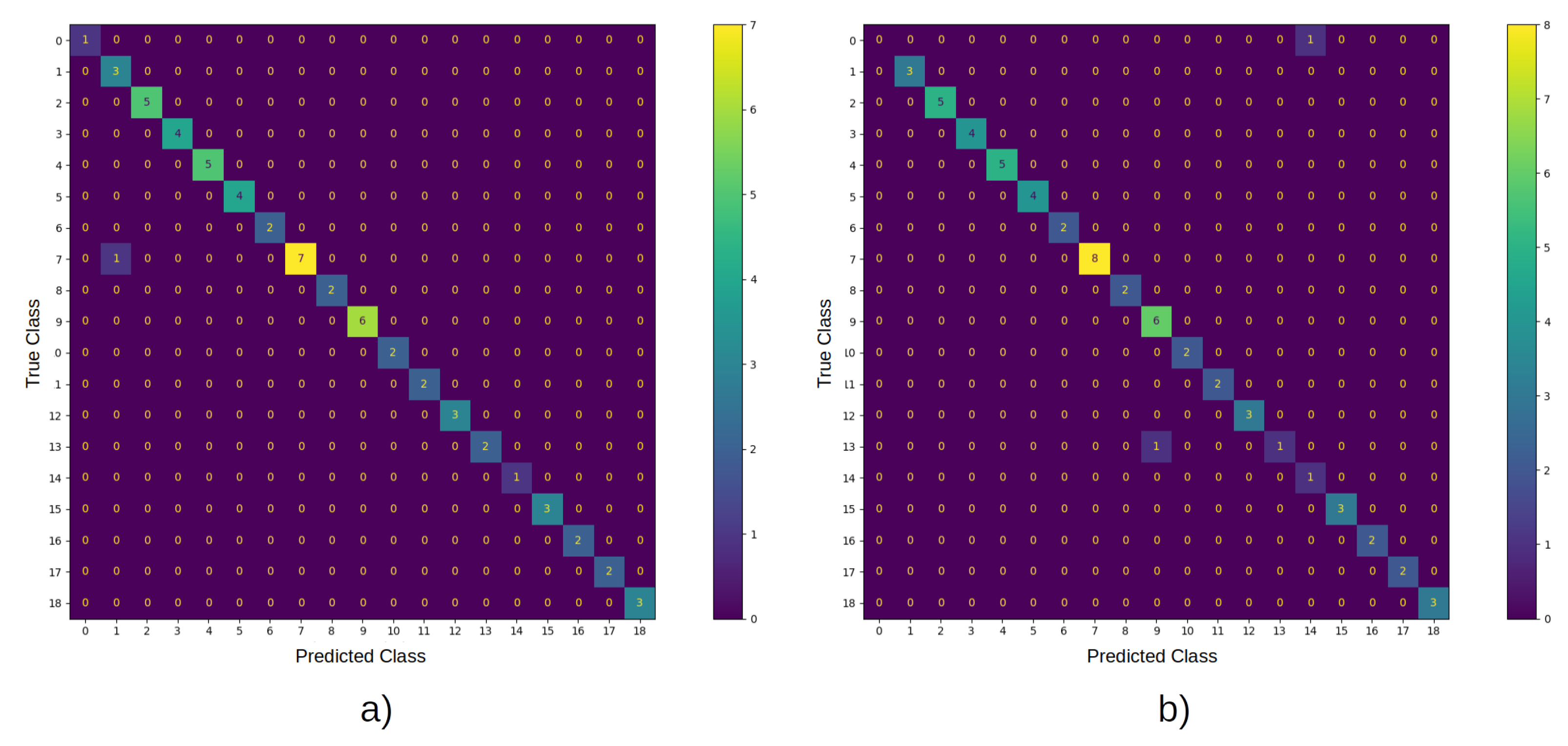
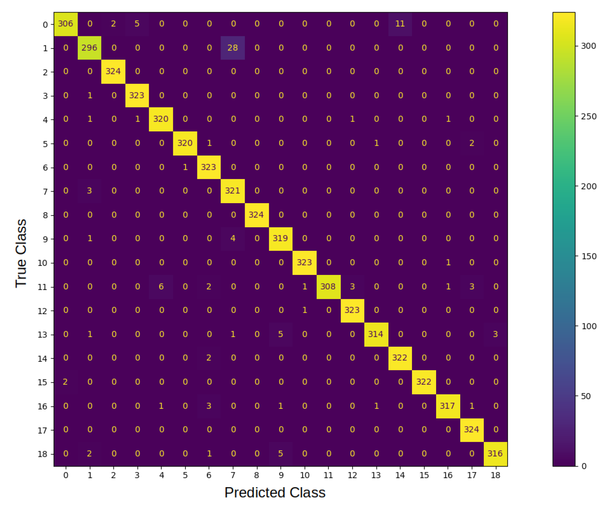
Analysis of the confusion matrix of the system implemented in Python (see Figure 8) showed that the classification errors of classes 0 and 1 were caused by the similarity of those objects in the computed view when $0^{\circ }<\theta <{20}^{\circ }$. In addition, the system on the FPGA had accuracy loss of 2%, which is quite acceptable in manufacturing; moreover, it is more than 655 times faster than its implementation on a PC.

The BOF has not been used before to extract information from an object from different angles and train a neural network. To validate this, we conducted a series of tests from which we demonstrated that using BOF instead of the image itself is a significant contribution.

In order to conduct a fair comparison between our proposal and state-of-the-art CNN models, we trained the latter with the image dataset that we had constructed for the case under study by feeding those CNN models with the images and their rotations in two described axes $\alpha$ and $\theta$.

CNNs are usually trained with datasets containing standard object classes (people, animals, vehicles, among others). In this contribution, however, we used the images obtained in Step 2 of the methodology (Section 2); we called it 3D Images Objects Dataset (3DIOD). Briefly, each image was segmented by selecting the region of interest of the object, scaled, and transformed into grayscale. With this, we formed the image dataset. Lastly, we trained two CNN models (ResNET50 [24] and MobileNetV2 [25]) with the image dataset. It was necessary to modify the output layer of one of them because the number of the classes changed to 19. The reason for choosing this CNN model was its relatively small size compared with that of. another CNN.

Table 13. Latency of several CNN models, their number of parameters, number of layers, and achieved accuracy using the dataset obtained in Step 2 of methodology.

CNN Model	Dataset	No. of Parameters	No. of Layers	Latency ∗ [ms]	Accuracy
ResNET50	3DIOD	23,626,643	50	118.02	97.9%
MobileNetV2	3DIOD	2,282,323	53	57.14	98.5%
Modified LeNet-5	3DBOFD	27,354	7	37.97	98.33%

* Latency mean for one sample.

shows the number of parameters, number of layers, average latency for classification, and accuracy for different known CNN models. This experiment was only programmed in Python and Keras.

From the results shown in the previous table, we can affirm that our hypothesis is valid. That is, our proposal (Modified LeNet-5 and BOF dataset) is faster and requires fewer parameters than those needed in ResNET50 or MobileNetV2 CNN models, which take raw images as their input data.

Table 14. Latency related work comparison for one classification.

	[13]		[14]	Our Work
Year	2021		2021	2022
Platform	XC7VX690T		XC7K325T	XC7Z020
Network	Mobilenet V2	Tiny YoloV3	Mobilenet V2	Modified LeNet-5
LUTs	279 K		146 K	31.3 K
BRAM	912		92	53
DSPs	3072		212	116
Classification latency [ms]	0.34	2.91	3.25	0.049

and

Table 15. Latency related work comparison for entire classification process.

			Our Work
	[27]	[16]	CPU	Zybo
Platform	Arria-10 GX1150	Zybo Z7-20 (XC7Z020)	Ryzen5 3400 G 16 GB	Zybo Z7-20 (XC7Z020)
Frecuency [MHz]	190	100	CPU@4200	100
Network	YOLOv2 Tiny	FAM	Modified LeNet-5	Modified LeNet-5
LUTs [K]	145 *	3.8	N/A	31.3
BRAM	1027 **	50	N/A	53
DSPs	1092	3	N/A	116
FPS	71.41	60	26.33	161.23
Latency [ms]	14	7.61	39	6.2
Power [W]	26	11.1	100	7
Price [USD] †	5520	199	736	199

† Approximated price found in the manufacture company website. * Logical cells are ALM. ** Converted to 36 Kb each.

shows the comparison of our FPGA implementation with the state-of-the-art models. We split the comparison because, in Table 14, the consumed time only shows the results for the classification process assuming that the image had been loaded on the FPGA. Meanwhile, in Table 15, the comparison is focused on fully implemented systems; the image was captured by a 60 FPS sensor and then transferred to the FPGA for inference.

Even though the cited works use images as input, the comparison is valid in contrast with our approach in which we feed BOF input as inputs. The reason for this is that the transfer of knowledge from the trained CNN models (shown in Table 13) to this FPGA implementation do not degrade the hardware performance.

The cited works in Table 14, Refs. [13,14], refer to an FPGA architecture for the MobilenetV2 and Tiny YoloV3 (modified YOLOV3 [26]) CNN models. The MobilNet V2 implemented in the first cited work is faster than the one implemented in the second, but at the cost of more consumed resources. Compared to these two systems, our work is faster and at the same time, requires far less parameters ti be trained.

Continuing with Table 15, the first of the cited works, Ref. [27], implemented a CNN model (YOLOv2 Tiny) directly in hardware. The second case listed in Table 15 is an implementation of BOF and Fuzzy ARTMAP in hardware. The same board was used, Zybo Z7-20. The dataset for this model consisted of 100 images of the objects of interest, one per category.

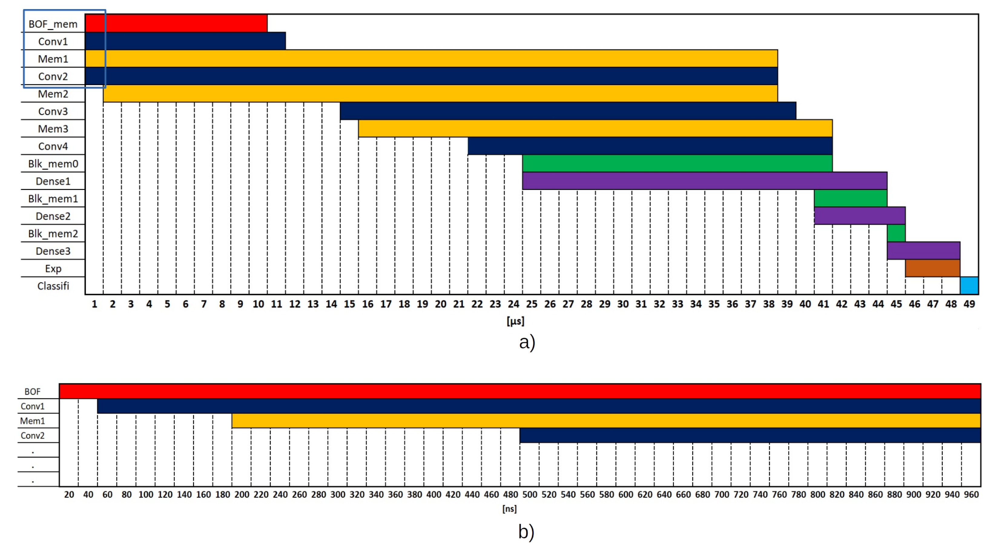
The latency in our model for classification is 0.04995 [ms]; however, loading the image in the FPGA takes 6.152 [ms]. Therefore, the total latency is 6.2 [ms] and 161.23 FPS. This result is 2.25X faster than [27]. The logic resources consumed in each project are remarkable; ours uses fewer LUTs, BRAMs and DSPs. The same is true for power consumption criteria and board price. Almost half of the XC7Z020 logic resources were used (LUTs, 58.90%; DSPs, 52.73%), so increasing the categories and image number is feasible.

5. Conclusions

Manufacturing requires adaptable systems that are able to cope with several configurations and orientations of components to be assembled. Real-time responses are a critical attribute in manufacturing systems, and conducting efforts to efficiently implement classifiers in hardware is, beyond doubt, a path that offers stable and reliable results. In this contribution, we described such a system and showed that results are encouraging and competitive compared to state-of-the-art solutions.

In this contribution, we proved that, in the robotic assembly context, the use of families of BOFs serving as input to convolutional neural networks leads to a faster and computationally more efficient training than the counterpart of using input multiview images as input to the vision system. We based our findings on a modified LeNet-5 CNN model. The results for the BOF case led to a latency of 37.97 ms for one inference and required 27,354 parameters, versus 57.14 ms and 2 million parameters for the multiple-view images. For the study case of interest in this contribution, both cases considered 19 classes of objects.

Continuing in the path of computational efficiency, the convolutional neural network implemented in FPGA could recognize relevant objects with high accuracy several times faster than its implementation in a general-purpose computer running Python, which is 655 times faster.

Compared with the literature on the state of the art, the latency for only one inference was 0.049 ms in our proposal (modified LeNet-5 trained with 3DBOFD) versus 0.34 ms in the cited work [13]. The latency for the entire process (capture the image and transfer the image to classify in the FPGA) took 6.2 ms, and in the cited work [27], it was 14 ms.

We opened a path to further investigate the impact of reliable hardware for implementing complex classifiers, such as convolutional neural networks, and achieve competitive results. We plan to extend the number of classes, and adjust and improve a larger CNN model as future work. We also plan to build a more comprehensive dataset for additional experiments with the most representative objects in assembly tasks.

References

1. Björnsson, A.; Jonsson, M.; Johansen, K. Automated material handling in composite manufacturing using pick-and-place systems—A review. Robot. Comput.-Integr. Manuf. 2018, 51, 222–229. [Google Scholar] [CrossRef]
2. Tella, R.; Birk, J.R.; Kelley, R.B. General Purpose Hands for Bin-Picking Robots. IEEE Trans. Syst. Man Cybern. 1982, 12, 828–837. [Google Scholar] [CrossRef]
3. Iriondo, A.; Lazkano, E.; Ansuategi, A. Affordance-based grasping point detection using graph convolutional networks for industrial bin-picking applications. Sensors 2021, 21, 816. [Google Scholar] [CrossRef] [PubMed]
4. Lopez-Juarez, I.; Howarth, M. Knowledge acquisition and learning in unstructured robotic assembly environments. Inf. Sci. 2002, 145, 89–111. [Google Scholar] [CrossRef]
5. Shih, C.L.; Lee, Y. A simple robotic eye-in-hand camera positioning and alignment control method based on parallelogram features. Robotics 2018, 7, 31. [Google Scholar] [CrossRef] [Green Version]
6. Fernandez, A.; Souto, A.; Gonzalez, C.; Mendez-Rial, R. Embedded vision system for monitoring arc welding with thermal imaging and deep learning. In Proceedings of the 2020 International Conference on Omni-Layer Intelligent Systems, COINS 2020, Barcelona, Spain, 31 August–2 September 2020. [Google Scholar] [CrossRef]
7. Herbert, B.; Andreas, E.; Tinne, T.; Gool, L.V. Speeded-Up Robust Features (SURF). Comput. Vis. Image Underst. 2008, 110, 346–359. [Google Scholar]
8. Cizek, P.; Faigl, J. Real-Time FPGA-Based Detection of Speeded-Up Robust Features Using Separable Convolution. IEEE Trans. Ind. Inform. 2018, 14, 1155–1163. [Google Scholar] [CrossRef]
9. Rosten, E.; Drummond, T. Machine learning for high-speed corner detection. Lect. Notes Comput. Sci. 2006, 3951 LNCS, 430–443. [Google Scholar] [CrossRef]
10. Calonder, M.; Lepetit, V.; Strecha, C.; Fua, P. BRIEF: Binary robust independent elementary features. Lect. Notes Comput. Sci. 2010, 6314 LNCS, 778–792. [Google Scholar] [CrossRef] [Green Version]
11. Ulusel, O.; Picardo, C.; Harris, C.B.; Reda, S.; Bahar, R.I. Hardware acceleration of feature detection and description algorithms on low-power embedded platforms. In Proceedings of the FPL 2016—26th International Conference on Field-Programmable Logic and Applications, Lausanne, Switzerland, 29 August–2 September 2016. [Google Scholar] [CrossRef]
12. Zhang, N.; Wei, X.; Chen, H.; Liu, W. FPGA implementation for CNN-based optical remote sensing object detection. Electronics 2021, 10, 282. [Google Scholar] [CrossRef]
13. Wu, C.; Zhuang, J.; Wang, K.; He, L. MP-OPU: A Mixed Precision FPGA-based Overlay Processor for Convolutional Neural Networks. In Proceedings of the 31st International Conference on Field-Programmable Logic and Applications (FPL), Dresden, Germany, 30 August–3 September 2021; pp. 33–37. [Google Scholar] [CrossRef]
14. Liu, P.; Song, Y. A hybrid vision processing unit with a pipelined workflow for convolutional neural network accelerating and image signal processing. Electronics 2021, 10, 2989. [Google Scholar] [CrossRef]
15. Mario, P.C.; Ismael, L.J.; Reyes, R.C.; Jorge, C.C. Machine vision approach for robotic assembly. Assem. Autom. 2005, 25, 204–216. [Google Scholar]
16. Lomas-Barrie, V.; Pena-Cabrera, M.; Lopez-Juarez, I.; Navarro-Gonzalez, J.L. Fuzzy artmap-based fast object recognition for robots using FPGA. Electronics 2021, 10, 361. [Google Scholar] [CrossRef]
17. Carpenter, G.A.; Grossberg, S.; Markuzon, N.; Reynolds, J.H.; Rosen, D.B. Fuzzy ARTMAP: A Neural Network Architecture for Incremental Supervised Learning of Analog Multidimensional Maps. IEEE Trans. Neural Netw. 1992, 3, 698–713. [Google Scholar] [CrossRef] [PubMed] [Green Version]
18. Sharma, A.; Vans, E.; Shigemizu, D.; Boroevich, K.A.; Tsunoda, T. DeepInsight: A methodology to transform a non-image data to an image for convolution neural network architecture. Sci. Rep. 2019, 9, 11399. [Google Scholar] [CrossRef] [PubMed] [Green Version]
19. Xiang, Z.; Zhao, J.; LeCun, Y. Character-level Convolutional Networks for Text Classification. In Advances in Neural Information Processing Systems 28 (NIPS 2015); MIT Press: Cambridge, MA, USA, 2013; pp. 3057–3061. Available online: http://xxx.lanl.gov/abs/1502.01710 (accessed on 8 January 2022).
20. Ankita, A.; Rani, S.; Bashir, A.K.; Alhudhaif, A.; Koundal, D.; Gunduz, E.S. An efficient CNN-LSTM model for sentiment detection in BlackLivesMatter. Expert Syst. Appl. 2022, 193, 116256. [Google Scholar] [CrossRef]
21. LeCun, Y.; Boser, B.; Denker, J.S.; Henderson, D.; Howard, R.E.; Hubbard, W.; Jackel, L.D. Backpropagation applied to digit recognition. Neural Comput. 1989, 1, 541–551. [Google Scholar] [CrossRef]
22. Devices, A. Fixed-Point vs. Floating-Point Digital Signal Processing. Available online: https://www.analog.com/en/technical-articles/fixedpoint-vs-floatingpoint-dsp.html (accessed on 8 January 2022).
23. Alcaraz, F.; Justin, J.; Eric, B. GitHub-Francof2a/Fxpmath: A Python Library for Fractional Fixed-Point (Base 2) Arithmetic and Binary Manipulation with Numpy Compatibility. Available online: https://github.com/francof2a/fxpmath#readme (accessed on 8 January 2022).
24. He, K.; Zhang, X.; Ren, S.; Sun, J. Deep residual learning for image recognition. In Proceedings of the IEEE Computer Society Conference on Computer Vision and Pattern Recognition, Las Vegas, NV, USA, 27–30 June 2016; pp. 770–778. Available online: http://xxx.lanl.gov/abs/1512.03385 (accessed on 8 January 2022). [CrossRef] [Green Version]
25. Sandler, M.; Howard, A.; Zhu, M.; Zhmoginov, A.; Chen, L.C. MobileNetV2: Inverted Residuals and Linear Bottlenecks. In Proceedings of the IEEE Computer Society Conference on Computer Vision and Pattern Recognition, Salt Lake City, UT, USA, 18–22 June 2018; pp. 4510–4520. Available online: http://xxx.lanl.gov/abs/1801.04381 (accessed on 8 January 2022). [CrossRef] [Green Version]
26. Redmon, J.; Farhadi, A. YOLOv3: An Incremental Improvement. 2018. Available online: http://arxiv.org/abs/1804.02767 (accessed on 8 January 2022).
27. Xu, K.; Wang, X.; Liu, X.; Cao, C.; Li, H.; Peng, H.; Wang, D. A dedicated hardware accelerator for real-time acceleration of YOLOv2. J. Real-Time Image Process. 2021, 18, 481–492. [Google Scholar] [CrossRef]
Figure 1. Obtaining the BOF dataset and training the network.
Electronics 11 00696 g001
Figure 2. Part recognition process implemented on hardware.
Electronics 11 00696 g002
Figure 3. (a) Example of manufacturing parts. (b) Studio.
Electronics 11 00696 g003
Figure 4. Camera angles.
Electronics 11 00696 g004
Figure 5. BOF extraction process for each object view.
Electronics 11 00696 g005
Figure 6. BOF and CNN FPGA implementation.
Electronics 11 00696 g006
Figure 7. Diagram of first convolution.
Electronics 11 00696 g007
Figure 8. Confusion matrix of CNN last version model.
Electronics 11 00696 g008
Figure 9. CNN diagram time performed in FPGA. (a) Whole process; (b) first μ s of the process.
Electronics 11 00696 g009
Figure 10. Confusion matrix of implemented CNN in (a) Python and (b) FPGA.
Electronics 11 00696 g010