
Energy-Efficient Respiratory Anomaly Detection in Premature Newborn Infants


Abstract
:1. Introduction
2. Related Work
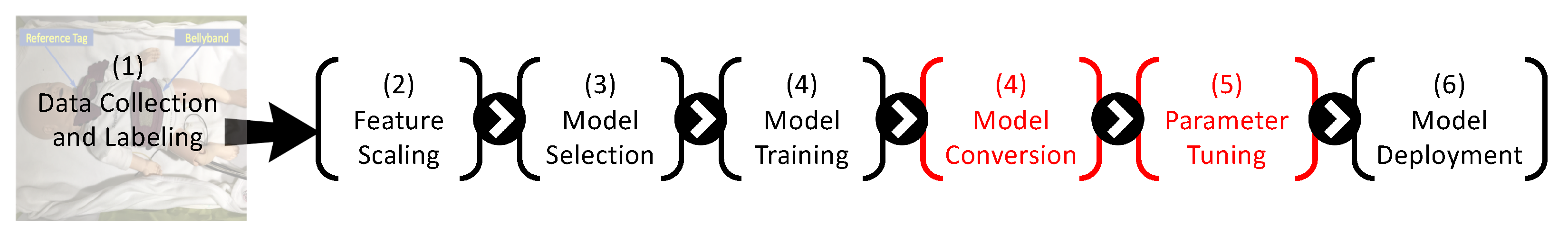
3. Design Pipeline
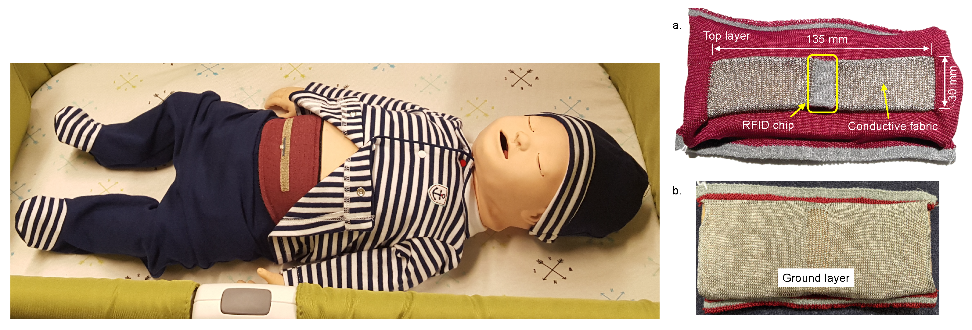
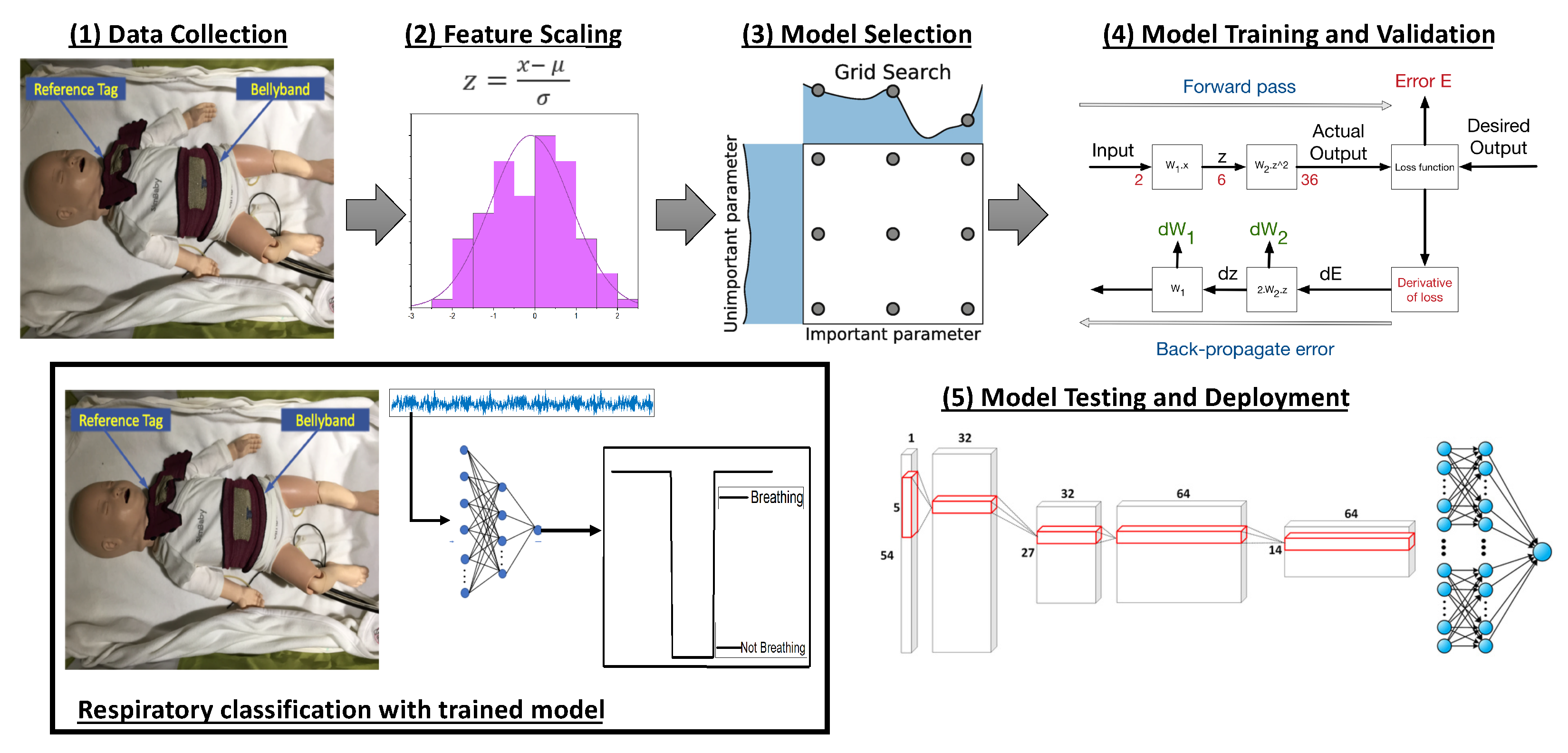
3.1. Data Collection and Labeling
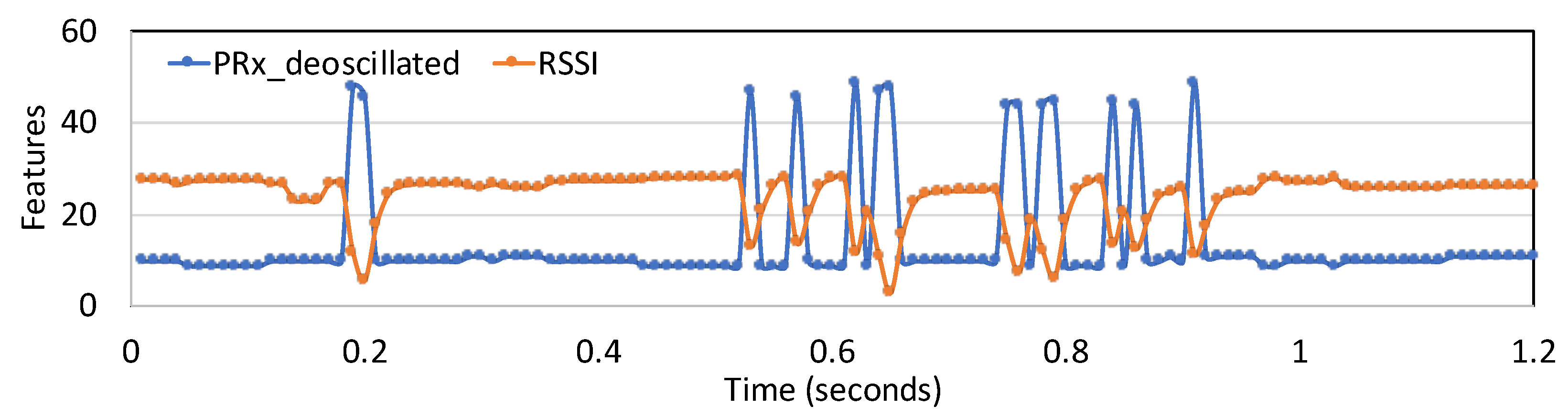
3.1.1. Data Collection and Feature Selection
- Feature 1: Reflected signal strength as measured at the interrogator, ()
- Feature 2: The difference between the current observed RSSI from the minimum RSSI value observed in the recent time window ()
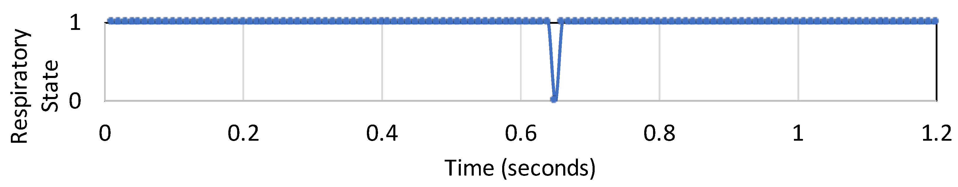
3.1.2. Data Labeling
3.2. Feature Scaling
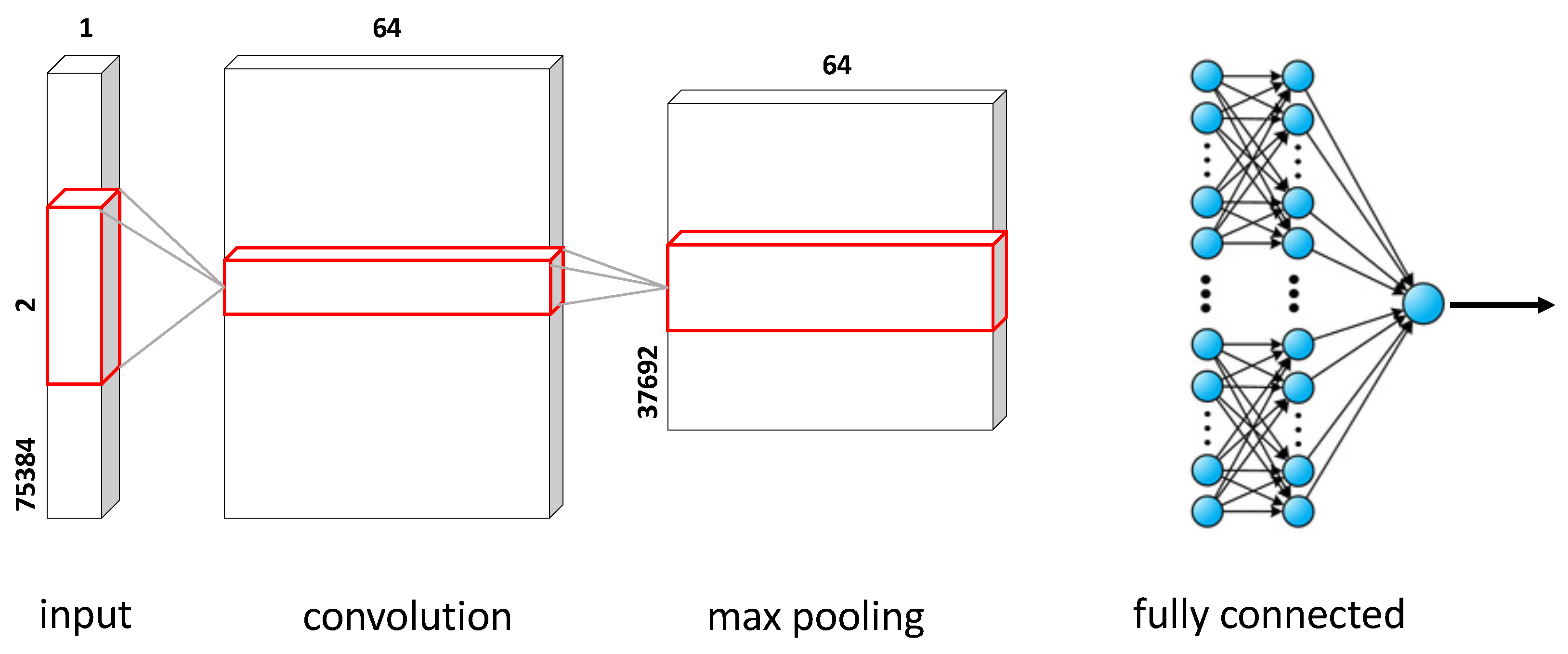
3.3. Deep Learning Model Selection
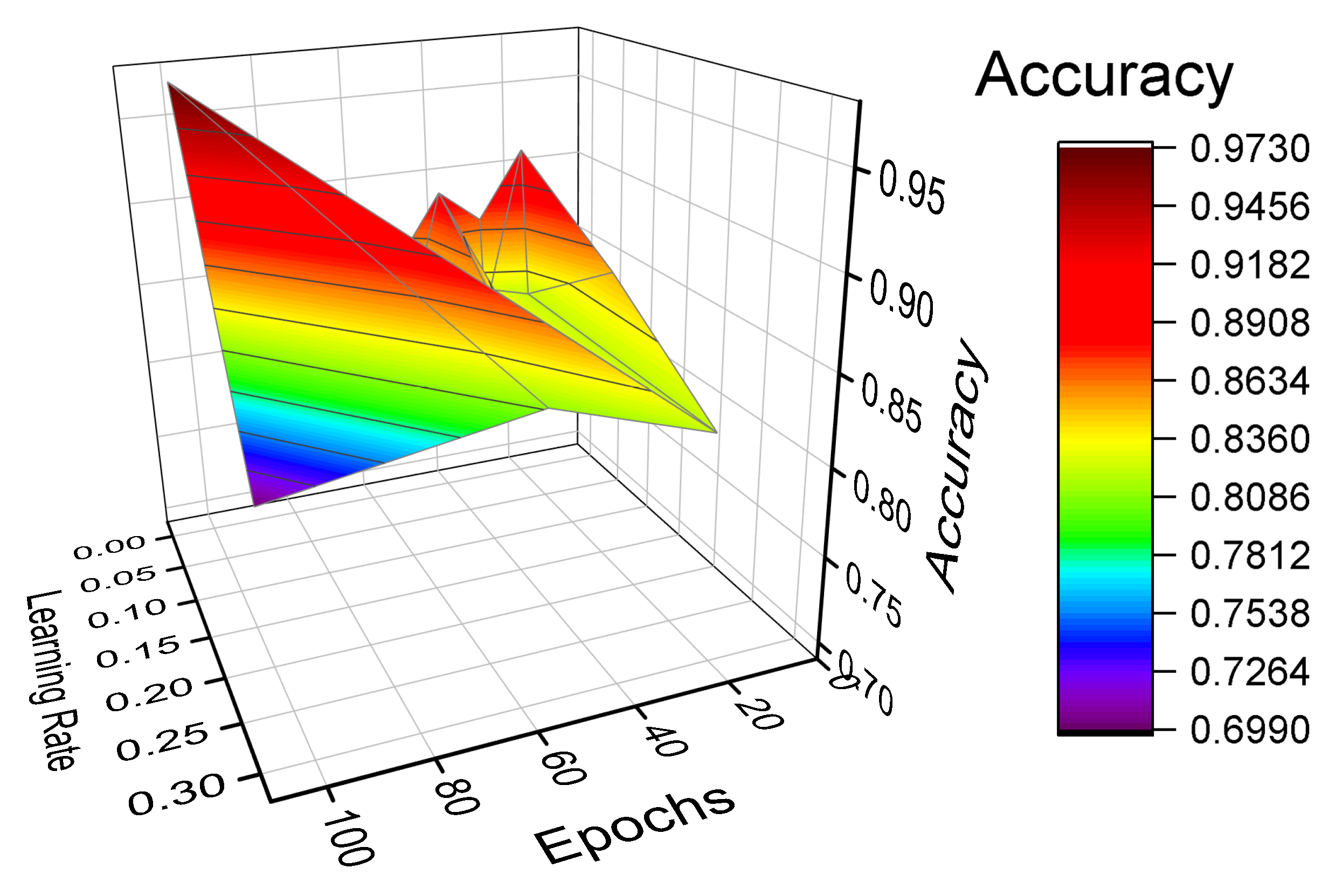
3.4. Hyperparameter Optimization
3.5. Model Training and Validation
3.6. Model Testing and Deployment
4. Model Quantization
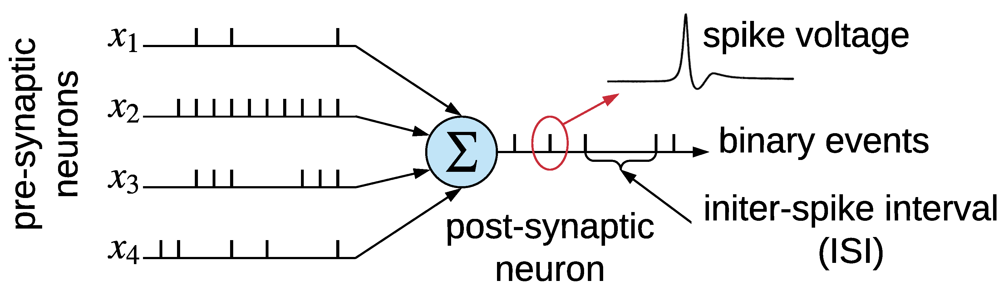
5. SNN-Based Respiratory Classification
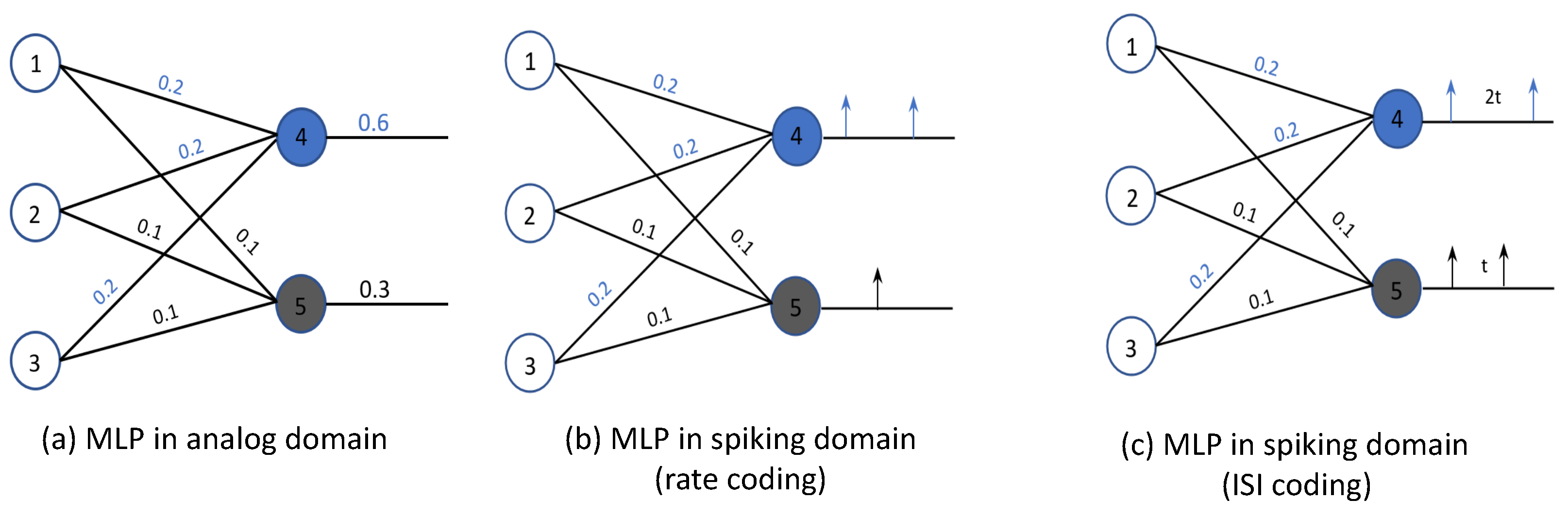
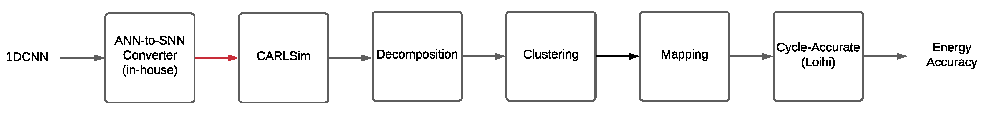
5.1. Model Conversion
- ReLU Activation Functions: This is implemented as the approximate firing rate of a leaky integrate and fire (LIF) neuron.
- Bias: A bias is represented as a constant input current to a neuron, the value of which is proportional to the bias of the neuron in the corresponding analog model.
- Weight Normalization: This is achieved by setting a factor to control the firing rate of spiking neurons.
- Softmax: To implement softmax, an external Poisson spike generator is used to generate spikes proportional to the weighted sum accumulated at each neuron.
- Max and Average Pooling: To implement max pooling, the neuron which fires first is considered to be the winning neuron, and therefore, its responses are forwarded to the next layer, suppressing the responses from other neurons in the pooling function. To implement average pooling, the average firing rate (obtained from total spike count) of the pooling neurons are forwarded to the next layer of the SNN.
- 1-D Convolution: The 1-D convolution is implemented to extract patterns from inputs in a single spacial dimension. A 1xn filter, called a kernel, slides over the input while computing the element-wise dot-product between the input and the kernel at each step.
- Residual Connections: Residual connections are implemented to convert the residual block used in CNN models such as ResNet. Typically, the residual connection connects the input of the residual block directly to the output neurons of the block, with a synaptic weight of ‘1’. This allows for the input to be directly propagated to the output of the residual block while skipping the operations performed within the block.
- Flattening: The flatten operation converts the 2-D output of the final pooling operation into a 1-D array. This allows for the output of the pooling operation to be fed as individual features into the decision-making fully connected layers of the CNN model.
- Concatenation: The concatenation operation, also known as a merging operation, is used as a channel-wise integration of the features extracted from two or more layers into a single output.
5.2. SNN Mapping to Neuromorphic Hardware
- Spike Data: the exact spike times of all neurons in the SNN model.
- Weight Data: the synaptic strength of all synapses in the SNN model.
5.3. SNN Parameter Tuning
6. Results and Discussions
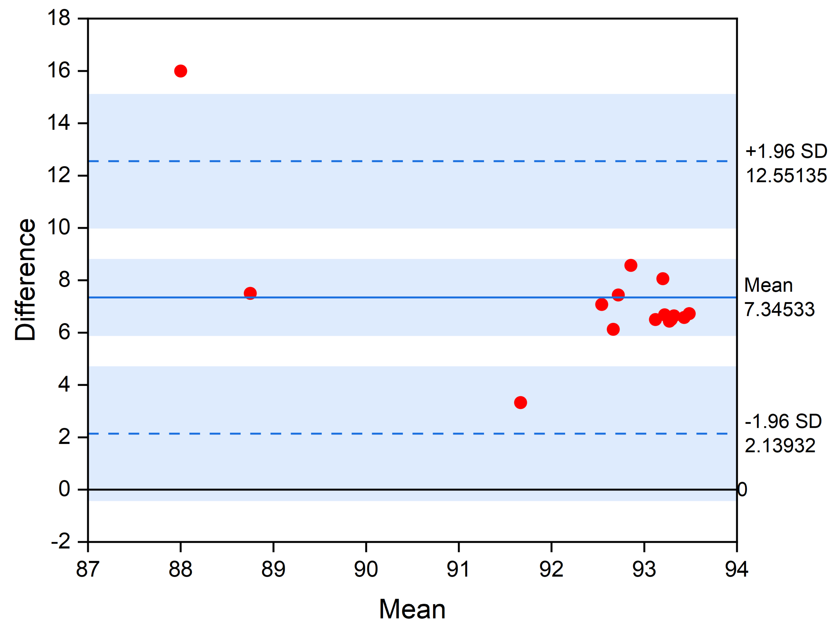
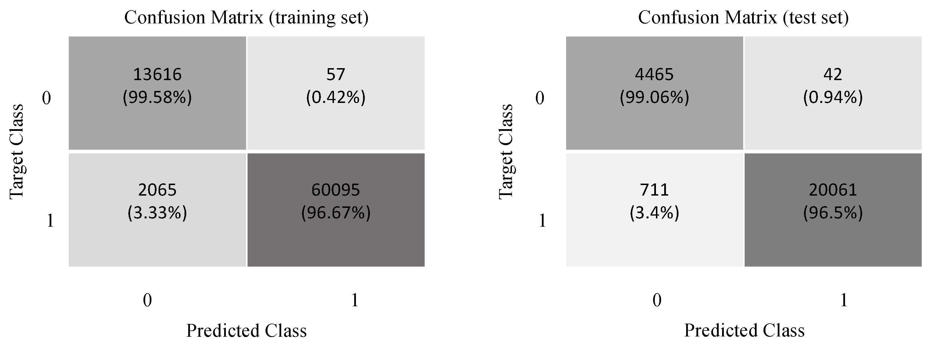
6.1. Baseline 1DCNN Performance
- Top-1 Accuracy: This is the conventional accuracy and it measures the proportion of test examples for which the predicted label (i.e., respiratory state) matches the expected label. To formulate top-1 accuracy, we introduce the following definitions.
- -
- True Positives (TP): For binary classification problems, i.e., ones with a yes/no outcome (such as the case of respiratory classification), this is the total number of test examples for which the value of the actual class is yes and the value of predicted class is also yes.
- -
- True Negatives (TN): This is the total number of test examples for which the value of the actual class is no and the value of the predicted class is also no.
- -
- False Positives (FP): This is the total number of test examples for which the value of the actual class is no but the value of the predicted class is yes.
- -
- False Negatives (FN): This is the total number of test examples for which the value of the actual class is yes but the value of the predicted class is no.
- F1 Score: To formulate the F1 score, we introduce the following definitions.
- -
- Precision: This is the ratio of correctly predicted positive observations to the total predicted positive observations, i.e.,
- -
- Recall: This is the ratio of correctly predicted positive observations to the all observations in actual class, i.e.,The F1 score conveys the balance between the precision and the recall. It is calculated as the weighted average of precision and recall, i.e.,
- AUC: In machine learning, a receiver operating characteristic (ROC) curve is a graphical plot that illustrates the diagnostic ability of a binary classifier as its discrimination threshold is varied. The area under curve (AUC) measures the two-dimensional area underneath the ROC curve. AUC tells how much the model is capable of distinguishing between classes. The higher the AUC, the better the model is at predicting yes classes as yes and no classes as no.
- Sensitivity: This is the true positive rate, i.e., how often the model correctly generates a yes out of all the examples for which the value of actual class is yes. Sensitivity is formulated as
- Specificity: This is the true negative rate, i.e., how often the model correctly generates a no out of all the examples for which the value of actual class is no. Specificity is formulated as
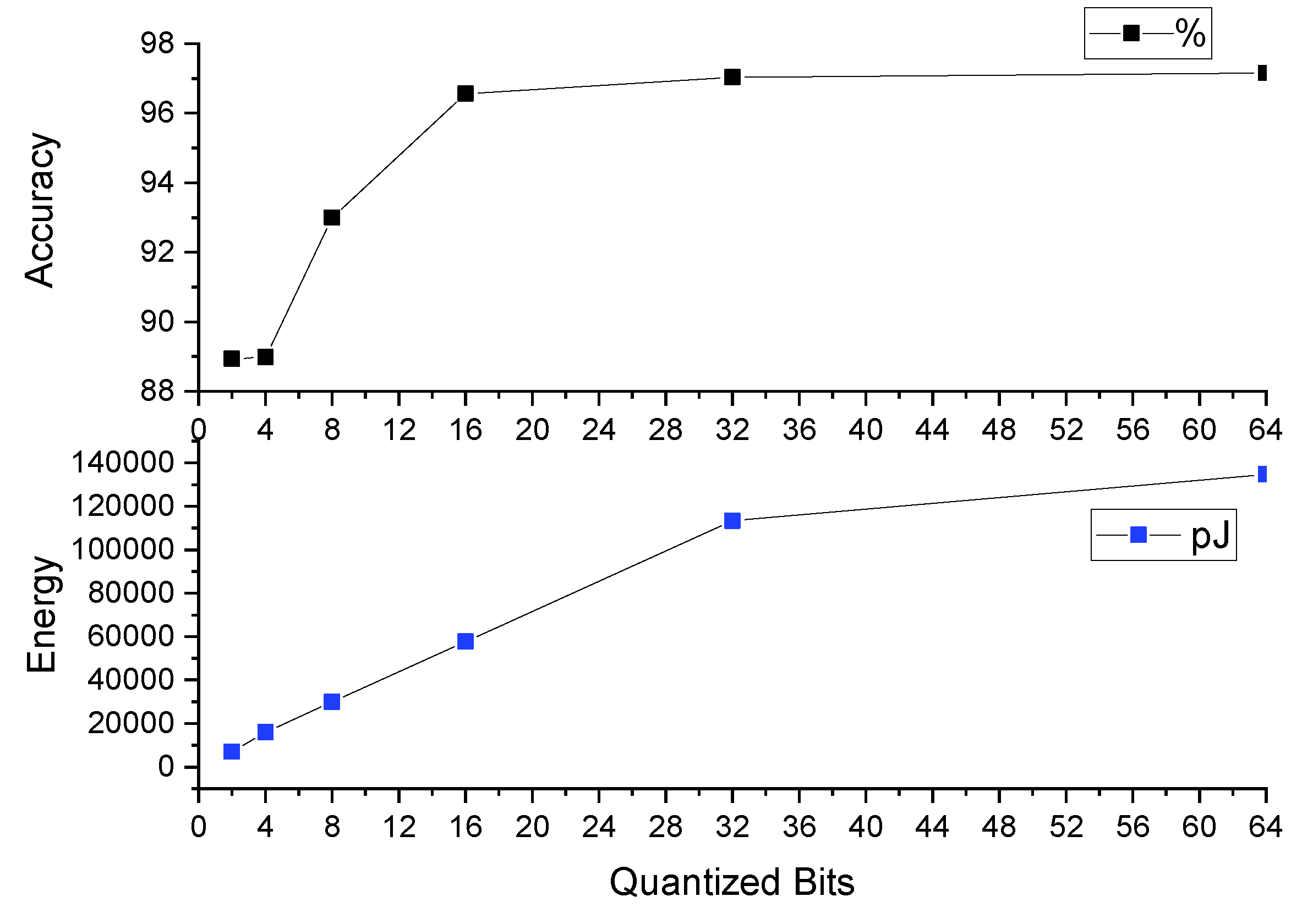
6.2. Quantization Results
6.3. SNN-Related Results
6.3.1. SNN Accuracy Compared to 1DCNN
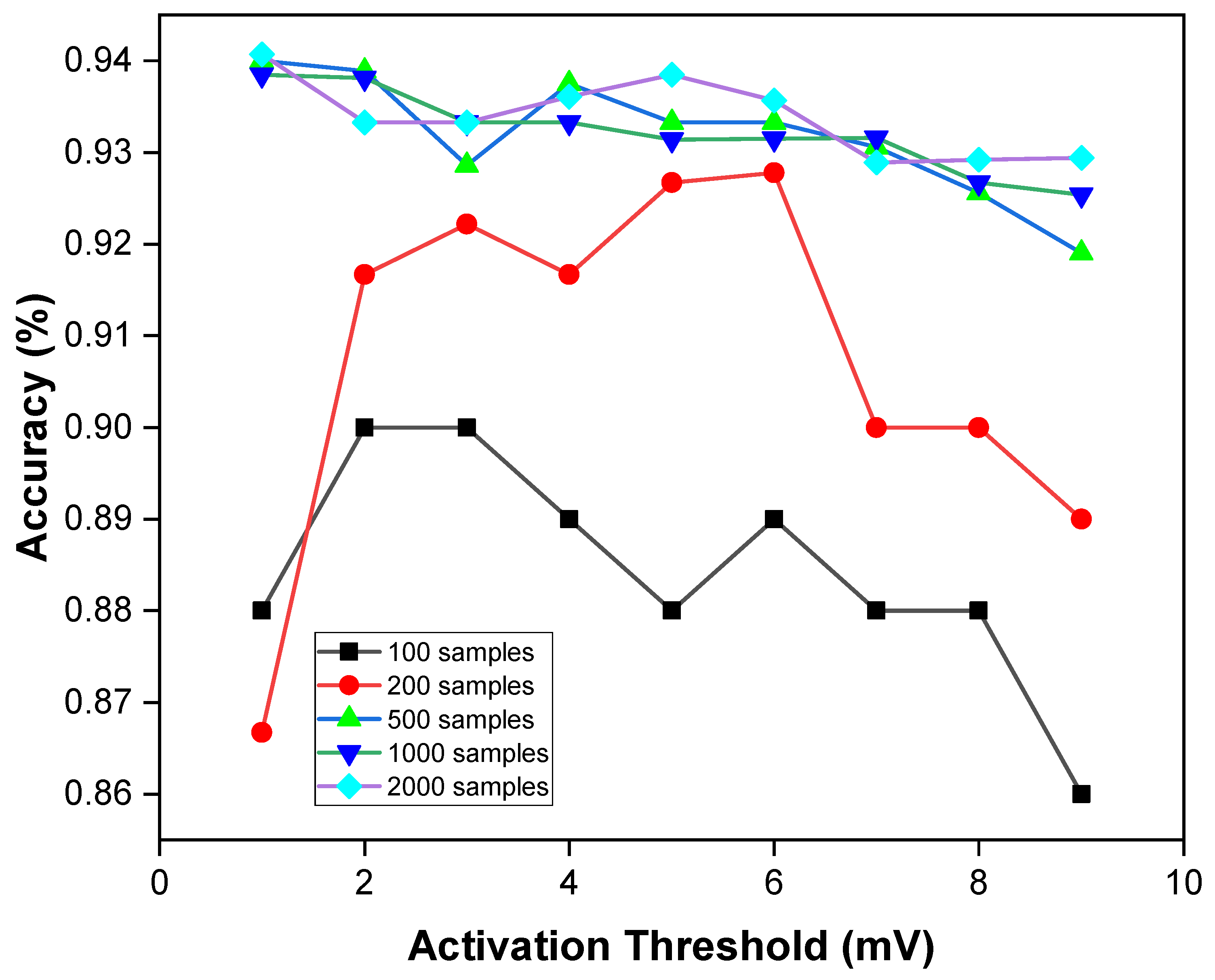
6.3.2. Design Space Exploration with SNN Parameters
7. Conclusions
Author Contributions
Funding
Institutional Review Board Statement
Informed Consent Statement
Conflicts of Interest
References
- Eichenwald, E.C.; Watterberg, K.L.; Aucott, S.; Benitz, W.E.; Cummings, J.J.; Goldsmith, J.; Poindexter, B.B.; Puopolo, K.; Stewart, D.L.; Wang, K.S. Apnea of Prematurity. Pediatrics 2016, 137, e20153757. [Google Scholar] [CrossRef] [PubMed] [Green Version]
- Clements, J.A.; Avery, M.E. Lung surfactant and neonatal respiratory distress syndrome. Am. J. Respir. Crit. Care Med. 1998, 157, S59–S66. [Google Scholar] [CrossRef] [PubMed]
- Rocha, G.; Soares, P.; Gonçalves, A.; Silva, A.I.; Almeida, D.; Figueiredo, S.; Pissarra, S.; Costa, S.; Soares, H.; Flôr-de Lima, F.; et al. Respiratory care for the ventilated neonate. Can. Respir. J. 2018, 2018, 7472964. [Google Scholar] [CrossRef] [PubMed] [Green Version]
- Antognoli, L.; Marchionni, P.; Nobile, S.; Carnielli, V.P.; Scalise, L. Assessment of cardio-respiratory rates by non-invasive measurement methods in hospitalized preterm neonates. In Proceedings of the 2018 IEEE International Symposium on Medical Measurements and Applications (MeMeA), Rome, Italy, 11–13 June 2018. [Google Scholar]
- Patron, D.; Mongan, W.; Kurzweg, T.P.; Fontecchio, A.; Dion, G.; Anday, E.K.; Dandekar, K.R. On the Use of Knitted Antennas and Inductively Coupled RFID Tags for Wearable Applications. IEEE Trans. Biomed. Circuits Syst. 2016, 10, 1047–1057. [Google Scholar] [CrossRef]
- Tajin, M.A.S.; Amanatides, C.E.; Dion, G.; Dandekar, K.R. Passive UHF RFID-based Knitted Wearable Compression Sensor. IEEE Internet Things J. 2021, 8, 13763–13773. [Google Scholar] [CrossRef]
- Mongan, W.; Anday, E.; Dion, G.; Fontecchio, A.; Joyce, K.; Kurzweg, T.; Liu, Y.; Montgomery, O.; Rasheed, I.; Sahin, C.; et al. A Multi-Disciplinary Framework for Continuous Biomedical Monitoring Using Low-Power Passive RFID-Based Wireless Wearable Sensors. In Proceedings of the 2016 IEEE International Conference on Smart Computing (SMARTCOMP), St. Louis, MO, USA, 18–20 May 2016. [Google Scholar]
- Ross, R.; Mongan, W.M.; O-Neill, P.; Rasheed, I.; Dion, G.; Dandekar, K.R. An Adaptively Parameterized Algorithm Estimating Respiratory Rate from a Passive Wearable RFID Smart Garment. In Proceedings of the 2021 IEEE 45th Annual Computers, Software, and Applications Conference (COMPSAC), Madrid, Spain, 12–16 July 2021. [Google Scholar]
- Vora, S.A.; Mongan, W.M.; Anday, E.K.; Dandekar, K.R.; Dion, G.; Fontecchio, A.K.; Kurzweg, T.P. On implementing an unconventional infant vital signs monitor with passive RFID tags. In Proceedings of the 2017 IEEE International Conference on RFID (RFID), Phoenix, AZ, USA, 9–11 May 2017. [Google Scholar]
- Gentry, A.; Mongan, W.; Lee, B.; Montgomery, O.; Dandekar, K.R. Activity Segmentation Using Wearable Sensors for DVT/PE Risk Detection. In Proceedings of the 2019 IEEE 43rd Annual Computer Software and Applications Conference (COMPSAC), Milwaukee, WI, USA, 15–19 July 2019. [Google Scholar]
- Tajin, M.A.S.; Mongan, W.M.; Dandekar, K.R. Passive RFID-based Diaper Moisture Sensor. Sensors 2020, 21, 1665–1674. [Google Scholar] [CrossRef]
- LeCun, Y.; Bengio, Y.; Hinton, G. Deep learning. Nature 2015, 521, 436–444. [Google Scholar] [CrossRef]
- Maass, W. Networks of spiking neurons: The third generation of neural network models. Neural Netw. 1997, 10, 1659–1671. [Google Scholar] [CrossRef]
- Debole, M.V.; Taba, B.; Amir, A.; Akopyan, F.; Andreopoulos, A.; Risk, W.P.; Kusnitz, J.; Otero, C.O.; Nayak, T.K.; Appuswamy, R.; et al. TrueNorth: Accelerating from zero to 64 million neurons in 10 years. Computer 2019, 52, 20–29. [Google Scholar] [CrossRef]
- Davies, M.; Srinivasa, N.; Lin, T.H.; Chinya, G.; Cao, Y.; Choday, S.H.; Dimou, G.; Joshi, P.; Imam, N.; Jain, S.; et al. Loihi: A neuromorphic manycore processor with on-chip learning. IEEE Micro 2018, 38, 82–99. [Google Scholar] [CrossRef]
- Moradi, S.; Qiao, N.; Stefanini, F.; Indiveri, G. A scalable multicore architecture with heterogeneous memory structures for dynamic neuromorphic asynchronous processors (DYNAPs). IEEE Trans. Biomed. Circuits Syst. 2017, 12, 106–122. [Google Scholar] [CrossRef] [PubMed] [Green Version]
- Gyselinckx, B.; Vullers, R.; Hoof, C.V.; Ryckaert, J.; Yazicioglu, R.F.; Fiorini, P.; Leonov, V. Human++: Emerging Technology for Body Area Networks. In Proceedings of the 2006 IFIP International Conference on Very Large Scale Integration, Nice, France, 16–18 October 2006. [Google Scholar] [CrossRef]
- Mongan, W.; Dandekar, K.; Dion, G.; Kurzweg, T.; Fontecchio, A. Statistical analytics of wearable passive RFID-based biomedical textile monitors for real-time state classification. In Proceedings of the 2015 IEEE Signal Processing in Medicine and Biology Symposium (SPMB), Philadelphia, PA, USA, 12 December 2015. [Google Scholar]
- Acharya, S.; Mongan, W.M.; Rasheed, I.; Liu, Y.; Anday, E.; Dion, G.; Fontecchio, A.; Kurzweg, T.; Dandekar, K.R. Ensemble learning approach via kalman filtering for a passive wearable respiratory monitor. IEEE J. Biomed. Health Inform. 2018, 23, 1022–1031. [Google Scholar] [CrossRef] [PubMed]
- Navaneeth, S.; Sarath, S.; Nair, B.A.; Harikrishnan, K.; Prajal, P. A deep-learning approach to find respiratory syndromes in infants using thermal imaging. In Proceedings of the 2020 International Conference on Communication and Signal Processing (ICCSP), Chennai, India, 28–30 July 2020. [Google Scholar]
- Basu, V.; Rana, S. Respiratory diseases recognition through respiratory sound with the help of deep neural network. In Proceedings of the 2020 4th International Conference on Computational Intelligence and Networks (CINE), Kolkata, India, 27–29 February 2020. [Google Scholar]
- Ravì, D.; Wong, C.; Deligianni, F.; Berthelot, M.; Andreu-Perez, J.; Lo, B.; Yang, G.Z. Deep learning for health informatics. IEEE J. Biomed. Health Inform. 2016, 21, 4–21. [Google Scholar] [CrossRef] [PubMed] [Green Version]
- Van Steenkiste, T.; Groenendaal, W.; Deschrijver, D.; Dhaene, T. Automated sleep apnea detection in raw respiratory signals using long short-term memory neural networks. IEEE J. Biomed. Health Inform. 2018, 23, 2354–2364. [Google Scholar] [CrossRef] [Green Version]
- Henaff, M.; Bruna, J.; LeCun, Y. Deep convolutional networks on graph-structured data. arXiv 2015, arXiv:1506.05163. [Google Scholar]
- Bejnordi, B.E.; Veta, M.; Van Diest, P.J.; Van Ginneken, B.; Karssemeijer, N.; Litjens, G.; Van Der Laak, J.A.; Hermsen, M.; Manson, Q.F.; Balkenhol, M.; et al. Diagnostic assessment of deep learning algorithms for detection of lymph node metastases in women with breast cancer. JAMA 2017, 318, 2199–2210. [Google Scholar] [CrossRef]
- Sannino, G.; De Pietro, G. A deep learning approach for ECG-based heartbeat classification for arrhythmia detection. Future Gener. Comput. Syst. 2018, 86, 446–455. [Google Scholar] [CrossRef]
- Das, A.; Pradhapan, P.; Groenendaal, W.; Adiraju, P.; Rajan, R.; Catthoor, F.; Schaafsma, S.; Krichmar, J.; Dutt, N.; Van Hoof, C. Unsupervised heart-rate estimation in wearables with Liquid states and a probabilistic readout. Neural Netw. 2018, 99, 134–147. [Google Scholar] [CrossRef] [Green Version]
- Balaji, A.; Corradi, F.; Das, A.; Pande, S.; Schaafsma, S.; Catthoor, F. Power-accuracy trade-offs for heartbeat classification on neural networks hardware. J. Low Power Electron. 2018, 14, 508–519. [Google Scholar] [CrossRef] [Green Version]
- Masquelier, T. Epileptic seizure detection using a neuromorphic-compatible deep spiking neural network. In Proceedings of the International Work-Conference on Bioinformatics and Biomedical Engineering, Granada, Spain, 8 May 2020. [Google Scholar]
- Su, Z.; Cheung, S.C.; Chu, K.T. Investigation of radio link budget for UHF RFID systems. In Proceedings of the 2010 IEEE International Conference on RFID-Technology and Applications, Guangzhou, China, 17–19 June 2010. [Google Scholar]
- Goodfellow, I.; Bengio, Y.; Courville, A. Deep Learning; MIT Press: London, UK, 2016. [Google Scholar]
- Bergstra, J.; Bengio, Y. Random search for hyper-parameter optimization. J. Mach. Learn. Res. 2012, 13, 28–305. [Google Scholar]
- Liu, X.; Li, W.; Huo, J.; Yao, L.; Gao, Y. Layerwise sparse coding for pruned deep neural networks with extreme compression ratio. In Proceedings of the AAAI Conference on Artificial Intelligence, New York, NY, USA, 7–12 February 2020. [Google Scholar]
- Choukroun, Y.; Kravchik, E.; Yang, F.; Kisilev, P. Low-bit Quantization of Neural Networks for Efficient Inference. In Proceedings of the ICCV Workshops, Seoul, Korea, 27 October–2 November 2019; pp. 3009–3018. [Google Scholar]
- Coelho, C.N.; Kuusela, A.; Li, S.; Zhuang, H.; Ngadiuba, J.; Aarrestad, T.K.; Loncar, V.; Pierini, M.; Pol, A.A.; Summers, S. Automatic heterogeneous quantization of deep neural networks for low-latency inference on the edge for particle detectors. Nat. Mach. Intell. 2021, 3, 675–686. [Google Scholar] [CrossRef]
- Gulli, A.; Pal, S. Deep Learning with Keras, 1st ed.; Packt Publishing: Birmingham, UK, 26 April 2017. [Google Scholar]
- Das, A.; Catthoor, F.; Schaafsma, S. Heartbeat classification in wearables using multi-layer perceptron and time-frequency joint distribution of ECG. In Proceedings of the 2018 IEEE/ACM International Conference on Connected Health: Applications, Systems and Engineering Technologies, New York, NY, USA, 26–28 September 2018. [Google Scholar]
- Dong, M.; Huang, X.; Xu, B. Unsupervised speech recognition through spike-timing-dependent plasticity in a convolutional spiking neural network. PLoS ONE 2018, 13, e0204596. [Google Scholar] [CrossRef] [PubMed]
- Sengupta, A.; Ye, Y.; Wang, R.; Liu, C.; Roy, K. Going deeper in spiking neural networks: VGG and residual architectures. Front. Neurosci. 2019, 13, 95. [Google Scholar] [CrossRef] [PubMed]
- Chou, T.; Kashyap, H.; Xing, J.; Listopad, S.; Rounds, E.; Beyeler, M.; Dutt, N.; Krichmar, J. CARLsim 4: An open source library for large scale, biologically detailed spiking neural network simulation using heterogeneous clusters. In Proceedings of the 2018 International Joint Conference on Neural Networks (IJCNN), Rio, Brazil, 8–13 July 2018. [Google Scholar]
- Balaji, A.; Song, S.; Titirsha, T.; Das, A.; Krichmar, J.; Dutt, N.; Shackleford, J.; Kandasamy, N.; Catthoor, F. NeuroXplorer 1.0: An Extensible Framework for Architectural Exploration with Spiking Neural Networks. In Proceedings of the International Conference on Neuromorphic Systems, Knoxville, TN, USA, 27–29 July 2021. [Google Scholar]
- Balaji, A.; Song, S.; Das, A.; Krichmar, J.; Dutt, N.; Shackleford, J.; Kandasamy, N.; Catthoor, F. Enabling Resource-Aware Mapping of Spiking Neural Networks via Spatial Decomposition. IEEE Embed. Syst. Lett. 2020, 13, 142–145. [Google Scholar] [CrossRef]
- Catthoor, F.; Mitra, S.; Das, A.; Schaafsma, S. Very large-scale neuromorphic systems for biological signal processing. In CMOS Circuits for Biological Sensing and Processing; Springer International Publishing: Berlin/Heidelberg, Germany, 2018. [Google Scholar]
- Liu, X.; Wen, W.; Qian, X.; Li, H.; Chen, Y. Neu-NoC: A high-efficient interconnection network for accelerated neuromorphic systems. In Proceedings of the 2018 23rd Asia and South Pacific Design Automation Conference (ASP-DAC), Jeju, Korea, 22–25 January 2018. [Google Scholar]
- Balaji, A.; Wu, Y.; Das, A.; Catthoor, F.; Schaafsma, S. Exploration of segmented bus as scalable global interconnect for neuromorphic computing. In Proceedings of the 2019 on Great Lakes Symposium on VLSI, Tysons Corner, VA, USA, 9–11 May 2019. [Google Scholar]
- Das, A.; Wu, Y.; Huynh, K.; Dell’Anna, F.; Catthoor, F.; Schaafsma, S. Mapping of local and global synapses on spiking neuromorphic hardware. In Proceedings of the 2018 Design, Automation & Test in Europe Conference & Exhibition (DATE), Dresden, Germany, 19–23 March 2018. [Google Scholar]
- Titirsha, T.; Song, S.; Balaji, A.; Das, A. On the Role of System Software in Energy Management of Neuromorphic Computing. In Proceedings of the 18th ACM International Conference on Computing Frontiers, Virtual Event, Italy, 11–13 May 2021. [Google Scholar]
- Balaji, A.; Das, A.; Wu, Y.; Huynh, K.; Dell’anna, F.G.; Indiveri, G.; Krichmar, J.L.; Dutt, N.D.; Schaafsma, S.; Catthoor, F. Mapping spiking neural networks to neuromorphic hardware. IEEE Trans. Very Large Scale Integr. (VLSI) Syst. 2020, 28, 76–86. [Google Scholar] [CrossRef]
- Song, S.; Balaji, A.; Das, A.; Kandasamy, N.; Shackleford, J. Compiling spiking neural networks to neuromorphic hardware. In Proceedings of the 21st ACM SIGPLAN/SIGBED Conference on Languages, Compilers, and Tools for Embedded Systems, London, UK, 16 June 2020. [Google Scholar]
- Das, A.; Kumar, A. Dataflow-Based Mapping of Spiking Neural Networks on Neuromorphic Hardware. In Proceedings of the 2018 on Great Lakes Symposium on VLSI, Chicago, IL, USA, 23–25 May 2018. [Google Scholar]
- Balaji, A.; Das, A. A Framework for the Analysis of Throughput-Constraints of SNNs on Neuromorphic Hardware. In Proceedings of the 2019 IEEE Computer Society Annual Symposium on VLSI (ISVLSI), Miami, FL, USA, 15–17 July 2019. [Google Scholar]
- Balaji, A.; Marty, T.; Das, A.; Catthoor, F. Run-time mapping of spiking neural networks to neuromorphic hardware. J. Signal Process. Syst. 2020, 92, 1293–1302. [Google Scholar] [CrossRef]
- Balaji, A.; Das, A. Compiling Spiking Neural Networks to Mitigate Neuromorphic Hardware Constraints. In Proceedings of the IGSC Workshops, Pullman, WA, USA, 19–22 October 2020. [Google Scholar]
- Titirsha, T.; Das, A. Thermal-Aware Compilation of Spiking Neural Networks to Neuromorphic Hardware. In Proceedings of the LCPC, New York, NY, USA, 14–16 October 2020. [Google Scholar]
- Song, S.; Das, A.; Kandasamy, N. Improving dependability of neuromorphic computing with non-volatile memory. In Proceedings of the EDCC, Munich, Germany, 7–10 September 2020. [Google Scholar]
- Song, S.; Hanamshet, J.; Balaji, A.; Das, A.; Krichmar, J.; Dutt, N.; Kandasamy, N.; Catthoor, F. Dynamic reliability management in neuromorphic computing. ACM J. Emerg. Technol. Comput. Syst. (JETC) 2021, 17, 1–27. [Google Scholar] [CrossRef]
- Song, S.; Das, A. A case for lifetime reliability-aware neuromorphic computing. In Proceedings of the MWSCAS, Springfield, MA, USA, 9–12 August 2020. [Google Scholar]
- Kundu, S.; Basu, K.; Sadi, M.; Titirsha, T.; Song, S.; Das, A.; Guin, U. Special Session: Reliability Analysis for ML/AI Hardware. In Proceedings of the VTS, San Diego, CA, USA, 25–28 April 2021. [Google Scholar]
- Song, S.; Das, A. Design Methodologies for Reliable and Energy-efficient PCM Systems. In Proceedings of the IGSC Workshops, Pullman, WA, USA, 19–22 October 2020. [Google Scholar]
- Titirsha, T.; Song, S.; Das, A.; Krichmar, J.; Dutt, N.; Kandasamy, N.; Catthoor, F. Endurance-Aware Mapping of Spiking Neural Networks to Neuromorphic Hardware. IEEE Trans. Parallel Distrib. Syst. 2021, 33, 288–301. [Google Scholar] [CrossRef]
- Titirsha, T.; Das, A. Reliability-Performance Trade-offs in Neuromorphic Computing. In Proceedings of the IGSC Workshops, Pullman, WA, USA, 19–22 October 2020. [Google Scholar]
- Song, S.; Titirsha, T.; Das, A. Improving Inference Lifetime of Neuromorphic Systems via Intelligent Synapse Mapping. In Proceedings of the 2021 IEEE 32nd International Conference on Application-specific Systems, Architectures and Processors (ASAP), Gothenburg, Sweden, 7–8 July 2021. [Google Scholar]
- Mallik, A.; Garbin, D.; Fantini, A.; Rodopoulos, D.; Degraeve, R.; Stuijt, J.; Das, A.; Schaafsma, S.; Debacker, P.; Donadio, G.; et al. Design-technology co-optimization for OxRRAM-based synaptic processing unit. In Proceedings of the 2017 Symposium on VLSI Technology, Kyoto, Japan, 5–8 June 2017. [Google Scholar]
- Abadi, M.; Barham, P.; Chen, J.; Chen, Z.; Davis, A.; Dean, J.; Devin, M.; Ghemawat, S.; Irving, G.; Isard, M.; et al. Tensorflow: A system for large-scale machine learning. In Proceedings of the 12th USENIX symposium on operating systems design and implementation (OSDI 16), Savannah, GA, USA, 2–4 November 2016. [Google Scholar]
- Coelho Jr, C.N.; Kuusela, A.; Zhuang, H.; Aarrestad, T.; Loncar, V.; Ngadiuba, J.; Pierini, M.; Summers, S. Ultra low-latency, low-area inference accelerators using heterogeneous deep quantization with QKeras and hls4ml. arXiv 2020, arXiv:2006.10159. [Google Scholar]


| Learning rate | 0.001 |
| Batch size | 5 |
| Optimizer | Adam |
| Data shuffle | per epoch |
| Maximum epochs | 100 |
| Neuron technology | 16 nm CMOS (original design is at 14 nm FinFET) |
| Synapse technology | HfO-based OxRRAM [63] |
| Supply voltage | 1.0 V |
| Energy per spike | 23.6 pJ at 30 Hz spike frequency |
| Energy per routing | 3 pJ |
| Switch bandwidth | 3.44 G. Events/s |
| Classification Technique | Top-1 Accuracy | F1 Score | AUC | Sensitivity | Specificity |
|---|---|---|---|---|---|
| SVM | 92.34% | 0.91 | 0.92 | 0.93 | 0.92 |
| LR | 91.60% | 0.91 | 0.90 | 0.90 | 0.92 |
| RF | 93.40% | 0.92 | 0.90 | 0.92 | 0.93 |
| 1DCNN (proposed) | 97.15% | 0.98 | 0.98 | 0.96 | 0.99 |
| Quantization | Top-1 Accuracy | Energy (pJ) | Model Size (bits) |
|---|---|---|---|
| 2-bit/parameter | 88.93% | 7089 | 92,258 |
| 4-bit/parameter | 88.98% | 15,994 | 184,516 |
| 8-bit/parameter | 93.00% | 29,871 | 369,032 |
| 16-bit/parameter | 96.55% | 57,640 | 738,064 |
| 32-bit/parameter | 97.03% | 113,386 | 1,476,128 |
| Baseline 1DCNN | 97.15% | 134,613 | 2,952,256 |
| Model | Top-1 Accuracy | Energy (pJ) |
|---|---|---|
| Baseline 1DCNN | 97.15% | 134,613 |
| 2-bit quantized 1DCNN | 88.93% | 7089 |
| 8-bit quantized 1DCNN | 93.00% | 29,871 |
| SNN | 93.33% | 7282 |
Publisher’s Note: MDPI stays neutral with regard to jurisdictional claims in published maps and institutional affiliations. |
© 2022 by the authors. Licensee MDPI, Basel, Switzerland. This article is an open access article distributed under the terms and conditions of the Creative Commons Attribution (CC BY) license (https://creativecommons.org/licenses/by/4.0/).
Share and Cite
Paul, A.; Tajin, M.A.S.; Das, A.; Mongan, W.M.; Dandekar, K.R. Energy-Efficient Respiratory Anomaly Detection in Premature Newborn Infants. Electronics 2022, 11, 682. https://doi.org/10.3390/electronics11050682
Paul A, Tajin MAS, Das A, Mongan WM, Dandekar KR. Energy-Efficient Respiratory Anomaly Detection in Premature Newborn Infants. Electronics. 2022; 11(5):682. https://doi.org/10.3390/electronics11050682
Chicago/Turabian StylePaul, Ankita, Md. Abu Saleh Tajin, Anup Das, William M. Mongan, and Kapil R. Dandekar. 2022. "Energy-Efficient Respiratory Anomaly Detection in Premature Newborn Infants" Electronics 11, no. 5: 682. https://doi.org/10.3390/electronics11050682
APA StylePaul, A., Tajin, M. A. S., Das, A., Mongan, W. M., & Dandekar, K. R. (2022). Energy-Efficient Respiratory Anomaly Detection in Premature Newborn Infants. Electronics, 11(5), 682. https://doi.org/10.3390/electronics11050682