Index Matrices—Based Software Implementation of Power Electronic Circuit Design

Abstract

This article aims to present a comprehensive approach with corresponding software that uses index matrices. They have been developed by the authors for an automated model-based design. One of the main goals of this paper is to propose a simple model solving technique for powering electronic devices (particularly, for all subsystems: power supplies, static power converters, electric filters, electrical loads, control systems, etc.). Index matrices, which contain first-order discrete dynamical system parameters, with real numbers as elements, are constructed in order so that voltages, amperages, and discrete values can be calculated. Simulations on a three-phase converter, as well as simulations on buck and boost DC-DC converters with PI controllers, are presented. The function of the proposed software (with examples on the aforementioned devices) is considered, and diagrams of its basic programming classes are shown. The latter draws electronic schemes and their respective graphics, and provides important characteristics. Simulink is used to verify results. Advantages of the proposed approach are a higher speed of calculations (compared to Simulink, due to a lack of differential equations) and a simpler handling of various electronic components. Additionally, a computational scalability is demonstrated.

1. Introduction

Techniques of solving differential equations solving are widely applied in software for model-based design of real-life systems. For example, power electronic components and devices are modeled in the libraries of one of the most popular graphical programming environments, Simulink, which uses a large number of simulation parameters and model solving modes [1,2]. Theoretically, many classes of dynamical systems can be represented by differential equations.

The first-order discrete dynamical systems have been described by linear systems, which concern consecutive time moments; there exist autonomous (time-independent) simple models (based on constant matrices), in which stability can be easy checked [3]. An example of the application of such a system on a DC-DC boost converter operation is demonstrated in [4]. Software implementations (see [5,6]) are useful with changing dependencies, because many estimations cannot be performed simply in this case; however, generally, power converters can be modeled with straightforward algorithms so that suitable simulations (based on non-constant matrices) can be performed [7,8,9].

The index matrices have arisen as extensions of the classical matrices. They provide a clear correspondence between elements and indices [10,11]. The index matrices represent a description tool for mathematical and real-life objects. The properties and applications of index matrices have been studied and summarized in [10]. The following types of their elements have been defined: integers, real numbers, Boolean values, predicates, fuzzy vales, etc., and additionally, three-dimensional index matrices have been introduced. Index matrices with real numbers as elements have been used by the authors in power electronic system modeling and simulation [6,12]; for example, single-ended primary-inductor converter example have been considered in [13].

Most of the results in the present paper are obtained by using the authors’ .NET software, with its features additionally considered in [5]. It automates the construction and solving of models based on index matrices. The graphics on electronic components (including on their time dependencies) in the presented software are similar to Simulink graphics, but the Simulink models and the proposed index matrix models differ significantly. Differential equations are used in Simulink, in which model configurations are relatively slow processes. The avoidance of the last ones is an important goal of the presented software, because the model-based design techniques, generally, require a large number of simulations (for example, as a part of optimization procedures). Such procedures can be performed faster with the proposed approach (since the linear systems are simpler than the differential equation systems, time-consuming model configurations are reduced).

2. Mathematical Methods and Models

Generally, all dynamical systems are simulated by estimating states at consecutive model time moments. The obtaining of values on system states (which usually are presented by one-dimensional or multidimensional arrays) is known as model solving [1]. No single solving method is optimal for all systems. For example, a typical power conversion system is constituted by subsystems, which have very different levels of detail [2]. Simulink provides a set of solvers, each of which uses a specific technique. According to the way in which the step size is calculated, they are divided into fixed-step and variable-step ones. The fixed-step solvers estimate values at regular model time intervals from the beginning to the end of the simulation. The step size can be specified, and it can be additionally chosen automatically. Generally, decreasing the step size increases the accuracy. The variable-step solvers vary the step size during the simulation. They reduce the step size to increase accuracy when model states are changing rapidly and increase the step size when model states are changing slowly. The approach, which is proposed in the present paper, uses a constant step size.

The apparatus of the indexed matrices (IMs) is not very popular. The respective concept was introduced in 1984 [14]. IMs have been used for a long time as an auxiliary tool for describing transitions of generalized nets only; their values are Boolean and predicate in case of conditions on token passes, and in integers in case of arc capacities [15,16,17]. Generalized nets are present in areas where modeling with Petri nets is not typical (for example, medicine and biotechnology). Indeed, it is impossible for generalized nets developed for their purposes to be replaced by Petri nets; the difference in the possibilities provided by the two formalisms is especially clear—the classes of tasks to be solved are completely different. The latter fact is also due to the use of IMs. Although basic properties of IMs have been studied in [10,11], a full review on their application is unpublished. Their usage in modeling of electrical circuits is very rare (an example is given in [18]), and their implementation requires additional training and the development of process automation software [19,20,21,22,23,24,25].

2.1. Basic Definitions on Index Matrices with Real Number Elements

Proper indices, which determine objects and features, cannot be included in classical matrices; usually respective identifiers are associated to columns of classical matrices. Since the classical matrices of different sizes cannot be summed, the index matrices operation ensures more compact representation. In similar way, there are no limitations on size of IMs in the case of their multiplication.

Generally, each index matrix with real numbers as elements (R-IM) has form

$$\overline{\mathrm{A}}=\langle \mathrm{K},\hspace{1em}\mathrm{L},\hspace{1em}{\left\{{\mathrm{a}}_{\mathrm{k},\mathrm{l}}\right\}}_{\mathrm{k}\in \mathrm{K}, \mathrm{l}\in \mathrm{L}}\subset ℝ\rangle ,$$

(1)

where

$$\mathrm{K}=\left\{{\mathrm{k}}_1, {\mathrm{k}}_2, \cdots ,{\mathrm{k}}_{\mathrm{m}}\right\},\hspace{1em}\mathrm{L}=\left\{{\mathrm{l}}_1, {\mathrm{l}}_2, \cdots ,{\mathrm{l}}_{\mathrm{n}}\right\},$$

(2)

are finite sets of indices [10,11]. In the present paper the following notation on the first and the second index sets of $\overline{\mathrm{A}}$ (K and L respectively) is used:

$${\mathrm{I}}_1\left(\overline{\mathrm{A}}\right)=\mathrm{K},{\mathrm{I}}_2\left(\overline{\mathrm{A}}\right)=\mathrm{L}.$$

(3)

The usual graphical representation of the above R-IM is

$$\overline{\mathrm{A}}=\begin{array}{ccccc}\underset{\_}{}\hfill & \underset{\_}{|{\mathrm{l}}_1}\hfill & \underset{\_}{{\mathrm{l}}_2}\hfill & \underset{\_}{{\cdots }_{ }}\hfill & \underset{\_}{{\mathrm{l}}_{\mathrm{n}}}\hfill \\ {\mathrm{k}}_1\hfill & |{\mathrm{a}}_{{\mathrm{k}}_1,{\mathrm{l}}_1}\hfill & {\mathrm{a}}_{{\mathrm{k}}_1,{\mathrm{l}}_2}\hfill & \cdots \hfill & {\mathrm{a}}_{{\mathrm{k}}_1,{\mathrm{l}}_{\mathrm{n}}}\hfill \\ {\mathrm{k}}_2\hfill & | {\mathrm{a}}_{{\mathrm{k}}_2,{\mathrm{l}}_1}\hfill & {\mathrm{a}}_{{\mathrm{k}}_2,{\mathrm{l}}_2}\hfill & \cdots & {\mathrm{a}}_{{\mathrm{k}}_2,{\mathrm{l}}_{\mathrm{n}}}\hfill \\ ⋮& {|\hspace{1em}⋮}^{}\hfill & ⋮& \ddots \hfill & ⋮\\ {\mathrm{k}}_{\mathrm{m}}\hfill & |{\mathrm{a}}_{{\mathrm{k}}_{\mathrm{m}},{\mathrm{l}}_1}\hfill & {\mathrm{a}}_{{\mathrm{k}}_{\mathrm{m}},{\mathrm{l}}_2}\hfill & \cdots & {\mathrm{a}}_{{\mathrm{k}}_{\mathrm{m}},{\mathrm{l}}_{\mathrm{n}}}\hfill \end{array}.$$

(4)

Here and below, all R-IMs are denoted by capital letters with additional lines (in order to be deferred from the classical matrices), and their elements by respective small letters. Each element of R-IM $\overline{\mathrm{A}}$ is in the same row with its index from ${\mathrm{I}}_1\left(\overline{\mathrm{A}}\right)$, and it is in the same column with its index from ${\mathrm{I}}_2\left(\overline{\mathrm{A}}\right)$. Lines divide indices from elements. Additionally, in (4), the considered indices are included as lower indices of elements of $\overline{\mathrm{A}}$. In all classical matrices, such lower indices are formed by row and column numbers.

Any swap of rows (or columns) of a classical matrix, which participates in a matrix equation, must correspond to a swap of rows (or columns) in other matrices from this equation in order that dependencies can be saved. Conversely, swaps of rows (or columns) in any index matrix do not change. In the context of the present paper, a R-IM on a resistor with resistance R can be represented by

$${\overline{\mathrm{F}}}_{\mathrm{R}}=\begin{array}{ccc}\underset{\_}{}& \underset{\_}{|{\mathrm{u}}_{\mathrm{R}}^{\mathrm{c}\mathrm{u}}}\hfill & \underset{\_}{{\mathrm{i}}_{\mathrm{R}}^{\mathrm{c}\mathrm{u}}}\\ {\mathrm{c}}_{\mathrm{R}}& |1\hfill & -\mathrm{R}\end{array}\equiv \begin{array}{ccc}\underset{\_}{}& \underset{\_}{|{\mathrm{i}}_{\mathrm{R}}^{\mathrm{c}\mathrm{u}}}\hfill & \underset{\_}{{\mathrm{u}}_{\mathrm{R}}^{\mathrm{c}\mathrm{u}}}\\ {\mathrm{c}}_{\mathrm{R}}& |-\mathrm{R}\hfill & 1\end{array}.$$

(5)

where ${\mathrm{u}}_{\mathrm{R}}^{\mathrm{c}\mathrm{u}}$ and ${\mathrm{i}}_{\mathrm{R}}^{\mathrm{c}\mathrm{u}}$ point to current voltage and current amperage respectively on the resistor. Let another R-IM

$$\overline{\mathrm{B}}=\langle \mathrm{P},\hspace{1em}\mathrm{Q},\hspace{1em}{\left\{{\mathrm{b}}_{\mathrm{p},\mathrm{q}}\right\}}_{\mathrm{p}\in \mathrm{P}, \mathrm{q}\in \mathrm{Q}}\rangle$$

(6)

be given. Sum (in index matrix theory the summation is denoted by “$\oplus$”)

$$\overline{\mathrm{C}}=\overline{\mathrm{A}}\oplus \overline{\mathrm{B}}=\left[\mathrm{K}\cup \mathrm{P},\hspace{1em}\mathrm{L}\cup \mathrm{Q},\hspace{1em}{\left\{{\mathrm{c}}_{\mathrm{r},\mathrm{s}}\right\}}_{\mathrm{r}\in \mathrm{K}\cup \mathrm{P}, \mathrm{s}\in \mathrm{L}\cup \mathrm{Q}}\right],$$

(7)

$${\mathrm{c}}_{\mathrm{r},\mathrm{s}}=\{\begin{array}{cc}{\mathrm{a}}_{\mathrm{r},\mathrm{s}},& \mathrm{i}\mathrm{f}\hspace{1em}\mathrm{r}\in {\mathrm{K}}_{{}_{{}_{{}_{{}_{{}_{}}}}}}\wedge \mathrm{s}\in \mathrm{L}-\mathrm{Q}\vee \mathrm{r}\in \mathrm{K}-\mathrm{P}\wedge \mathrm{s}\in \mathrm{L};\\ {\mathrm{b}}_{\mathrm{r},\mathrm{s}},& \mathrm{i}\mathrm{f}\hspace{1em}\mathrm{r}\in {\mathrm{P}}_{{}_{{}_{{}_{{}_{{}_{}}}}}}\wedge \mathrm{s}\in \mathrm{Q}-\mathrm{L}\vee \mathrm{r}\in \mathrm{P}-\mathrm{K}\wedge \mathrm{s}\in \mathrm{Q};\\ {\mathrm{a}}_{\mathrm{r},\mathrm{s}}+{\mathrm{b}}_{\mathrm{r},\mathrm{s}},& \mathrm{i}\mathrm{f}\hspace{1em}\mathrm{r}\in \mathrm{K}\cap {\mathrm{P}}_{{}_{{}_{{}_{{}_{{}_{}}}}}}\wedge \mathrm{s}\in \mathrm{L}\cap \mathrm{Q};\\ 0,& \mathrm{o}\mathrm{t}\mathrm{h}\mathrm{e}\mathrm{r}\mathrm{w}\mathrm{i}\mathrm{s}\mathrm{e};\end{array}$$

(8)

is a R-IM too. А sum of two index matrices, which have form (5), is presented below:

$$\begin{array}{ccc}\underset{\_}{}& \underset{\_}{|{\mathrm{u}}_{{\mathrm{R}}_1}^{\mathrm{c}\mathrm{u}}}\hfill & \underset{\_}{{\mathrm{i}}_{{\mathrm{R}}_1}^{\mathrm{c}\mathrm{u}}}\\ {\mathrm{c}}_{{\mathrm{R}}_1}& |1\hfill & -{\mathrm{R}}_1\end{array}\oplus \begin{array}{ccc}\underset{\_}{}& \underset{\_}{|{\mathrm{u}}_{{\mathrm{R}}_2}^{\mathrm{c}\mathrm{u}}}\hfill & \underset{\_}{{\mathrm{i}}_{{\mathrm{R}}_2}^{\mathrm{c}\mathrm{u}}}\\ {\mathrm{c}}_{{\mathrm{R}}_2}& |1\hfill & -{\mathrm{R}}_2\end{array}=\begin{array}{ccccc}\underset{\_}{}& \underset{\_}{|{\mathrm{u}}_{{\mathrm{R}}_1}^{\mathrm{c}\mathrm{u}}}\hfill & \underset{\_}{{\mathrm{i}}_{{\mathrm{R}}_1}^{\mathrm{c}\mathrm{u}}}& \underset{\_}{{\mathrm{u}}_{{\mathrm{R}}_2}^{\mathrm{c}\mathrm{u}}}& \underset{\_}{{\mathrm{i}}_{{\mathrm{R}}_2}^{\mathrm{c}\mathrm{u}}}\\ {\mathrm{c}}_{{\mathrm{R}}_1}& |1\hfill & -{\mathrm{R}}_1& 0& 0\\ {\mathrm{c}}_{{\mathrm{R}}_2}& |0\hfill & 0& 1& -{\mathrm{R}}_2\end{array}.$$

(9)

Since classical matrices of different sizes cannot be summed, it is obvious that in the case of their usage in matrix equations such compact expressions cannot be obtained. The following example supports the last assertion:

$$\left(\begin{array}{cccc}1& -{\mathrm{R}}_1& 0& 0\\ 0& 0& 0& 0\end{array}\right)+\left(\begin{array}{cccc}0& 0& 0& 0\\ 0& 0& 1& -{\mathrm{R}}_2\end{array}\right)=\left(\begin{array}{cccc}1& -{\mathrm{R}}_1& 0& 0\\ 0& 0& 1& -{\mathrm{R}}_2\end{array}\right).$$

(10)

Indices, which point to resistors, and voltages and amperages, cannot be included in (10); usually, identifiers are associated to the columns in such matrix equations.

In [10,11] a product of R-IMs (their multiplication is denoted by “$\odot$”) is defined. In case of index matrices $\overline{\mathrm{A}}$ and $\overline{\mathrm{B}}$:

$$\overline{\mathrm{D}}=\overline{\mathrm{A}}\odot \overline{\mathrm{B}}=\langle \mathrm{K}\cup \left(\mathrm{P}-\mathrm{L}\right),\hspace{1em}\mathrm{Q}\cup \left(\mathrm{L}-\mathrm{P}\right),\hspace{1em}{\left\{{\mathrm{d}}_{\mathrm{r},\mathrm{s}}\right\}}_{\mathrm{r}\in \mathrm{K}\cup \left(\mathrm{P}-\mathrm{L}\right), \mathrm{s}\in \mathrm{Q}\cup \left(\mathrm{L}-\mathrm{P}\right)}\rangle ,$$

(11)

$${\mathrm{d}}_{\mathrm{r},\mathrm{s}}=\{\begin{array}{cc}{\mathrm{a}}_{\mathrm{r},\mathrm{s}},& \mathrm{i}\mathrm{f}\hspace{1em}\mathrm{r} \in {\mathrm{K}}_{{}_{{}_{{}_{{}_{{}_{}}}}}}\wedge \mathrm{s} \in \mathrm{L}-\mathrm{P}-\mathrm{Q}; \\ {\mathrm{b}}_{\mathrm{r},\mathrm{s}},& \mathrm{i}\mathrm{f}\hspace{1em}\mathrm{r} \in \mathrm{P}-\mathrm{K}-{\mathrm{L}}_{{}_{{}_{}}}\wedge \mathrm{s} \in \mathrm{Q};\\ {\displaystyle \sum _{\mathrm{t}\in \mathrm{L}\cap \mathrm{P}}{\mathrm{a}}_{\mathrm{r},\mathrm{t}}{\mathrm{b}}_{\mathrm{t},\mathrm{s}} ,}& \mathrm{i}\mathrm{f}\hspace{1em}\mathrm{r} \in {\mathrm{K}}_{{}_{{}_{{}_{{}_{{}_{{}_{{}_{{}_{{}_{{}_{{}_{{}_{}}}}}}}}}}}}}\wedge \mathrm{s} \in \mathrm{Q};\\ 0,& \mathrm{o}\mathrm{t}\mathrm{h}\mathrm{e}\mathrm{r}\mathrm{w}\mathrm{i}\mathrm{s}\mathrm{e}.\end{array}$$

(12)

The last sum has a well-known analog in classical matrices theory; in case of $\mathrm{L}\equiv \mathrm{P}$ such sums are calculated for all elements of $\overline{\mathrm{A}}\odot \overline{\mathrm{B}}$ (see (10)), i.e.,

$$\begin{array}{cc}\begin{array}{cc}\mathrm{L}\equiv \mathrm{P}& \Rightarrow \end{array}& \left(\overline{\mathrm{D}}=\overline{\mathrm{A}}\odot \overline{\mathrm{B}}=\langle \mathrm{K},\hspace{1em}\mathrm{Q},\hspace{1em}{\left\{{\mathrm{d}}_{\mathrm{r},\mathrm{s}}\right\}}_{\mathrm{r}\in \mathrm{K}, \mathrm{s}\in \mathrm{Q}}\rangle ,\hspace{1em}{\mathrm{d}}_{\mathrm{r},\mathrm{s}}={\displaystyle \sum _{\mathrm{t}\in \mathrm{L}\equiv \mathrm{P}}{\mathrm{a}}_{\mathrm{r},\mathrm{t}}{\mathrm{b}}_{\mathrm{t},\mathrm{s}}}\right) .\end{array}$$

(13)

For each multiplication in the present paper, the second index set of its first R-IM is a subset of the first index set of its second R-IM, and the second index set of its second R-IM has one element, denoted by $\mathrm{o}$, only. In case of $\overline{\mathrm{A}}$ and $\overline{\mathrm{B}}$ it means that $\mathrm{L}\subseteq \mathrm{P}$ and $\mathrm{Q}=\left\{\mathrm{o}\right\}$; the following statement holds:

$$\begin{array}{cc}\begin{array}{cc}\left(\mathrm{L}\equiv \mathrm{P}\wedge \mathrm{Q}=\left\{\mathrm{o}\right\}\right)& \Rightarrow \end{array}& (\overline{\mathrm{D}}=\overline{\mathrm{A}}\odot \overline{\mathrm{B}}=\langle \mathrm{K}\cup \left(\mathrm{P}-\mathrm{L}\right),\hspace{1em}\left\{\mathrm{o}\right\},\hspace{1em}{\left\{{\mathrm{d}}_{\mathrm{r},\mathrm{o}}\right\}}_{\mathrm{r}\in \mathrm{K}\cup \left(\mathrm{P}-\mathrm{L}\right)}\rangle ,\end{array}$$

(14)

$${\mathrm{d}}_{\mathrm{r},\mathrm{o}}=\{\begin{array}{cc}{\mathrm{b}}_{\mathrm{r},\mathrm{o}},& \mathrm{i}{\mathrm{f}}_{{}_{{}_{{}_{}}}}\hspace{1em}\mathrm{r} \notin \mathrm{K};\\ {\displaystyle \sum _{\mathrm{t}\in \mathrm{L}}{\mathrm{a}}_{\mathrm{r},\mathrm{t}}{\mathrm{b}}_{\mathrm{t},\mathrm{o}},}& \mathrm{o}\mathrm{t}\mathrm{h}\mathrm{e}\mathrm{r}\mathrm{w}\mathrm{i}\mathrm{s}\mathrm{e}.\end{array}).$$

(15)

An example is given below:

$$\begin{array}{ccc}\underset{\_}{}& \underset{\_}{|{\mathrm{u}}_{\mathrm{R}}^{\mathrm{c}\mathrm{u}}}\hfill & \underset{\_}{{\mathrm{i}}_{\mathrm{R}}^{\mathrm{c}\mathrm{u}}}\\ {\mathrm{c}}_{\mathrm{R}}& |1\hfill & -\mathrm{R}\end{array}\odot \begin{array}{cc}\underset{\_}{}& \underset{\_}{|\mathrm{o}}\hfill \\ {\mathrm{u}}_{\mathrm{R}}^{\mathrm{c}\mathrm{u}}& |{\mathrm{u}}_{\mathrm{R}}^{}\left(\mathrm{t}\right)\hfill \\ {\mathrm{i}}_{\mathrm{R}}^{\mathrm{c}\mathrm{u}}& |{\mathrm{i}}_{\mathrm{R}}^{}\left(\mathrm{t}\right)\hfill \\ {\mathrm{u}}_E^{\mathrm{c}\mathrm{u}}& |{\mathrm{u}}_E^{}\left(\mathrm{t}\right)\hfill \end{array}=\begin{array}{cc}\underset{\_}{}& \underset{\_}{|\mathrm{o}}\hfill \\ {\mathrm{c}}_{\mathrm{R}}^{}& |{\mathrm{u}}_{\mathrm{R}}^{}\left(\mathrm{t}\right)-\mathrm{R} {\mathrm{i}}_{\mathrm{R}}^{}\left(\mathrm{t}\right)\hfill \\ {\mathrm{u}}_E^{\mathrm{c}\mathrm{u}}& |{\mathrm{u}}_E^{}\left(\mathrm{t}\right)\hfill \end{array}.$$

(16)

The elements of the first R-IM are coefficients of linear dependency; the elements of the second R-IM—voltage or amperage values; and the elements of the third R-IM—resultant values. In the third R-IM, one element is a linear combination and one element (which can be considered as constant voltage in ideal DC voltage source) remains unchanged (index ${\mathrm{u}}_{\mathrm{E}}^{\mathrm{c}\mathrm{u}}$ is not presented in set ${\mathrm{I}}_2\left({\overline{\mathrm{F}}}_{\mathrm{R}}\right)$).

2.2. Classical Matrix Models on First-Order Discrete Dynamical Systems

In [3] a time-independent first-order discrete dynamical system is defined by

$$X\left(\mathrm{t}+\Delta \mathrm{t}\right)=\mathrm{A}X\left(\mathrm{t}\right)+\mathrm{B},\hspace{1em}\hspace{1em}X\left(\mathrm{t}\right)={\left[\begin{array}{cccc}{x}_1\left(\mathrm{t}\right)& x_2\left(\mathrm{t}\right)& \dots & x_{\mathrm{n}}\left(\mathrm{t}\right)\end{array}\right]}^{\mathrm{T}},$$

(17)

where matrices $\mathrm{A}$ and $\mathrm{B}$ are constant, and

$$\mathrm{t}\in \mathrm{\Theta }\equiv \left\{\begin{array}{cccc}{\mathrm{t}}_0,& {\mathrm{t}}_0+\Delta {\mathrm{t}}_{ },& {\mathrm{t}}_0+2\Delta {\mathrm{t}}_{ },& \dots \end{array}\right\},\hspace{1em}\hspace{1em}{\mathrm{t}}_0,\Delta \mathrm{t}\in ℝ,\hspace{1em}\hspace{1em}\Delta \mathrm{t}=\frac{1}{{\mathrm{F}}_{\mathrm{d}}}>0.$$

(18)

Here time set $\Theta$ has sampling step $\Delta \mathrm{t}$ and discretization frequency ${\mathrm{F}}_{\mathrm{d}}$. State vector $\mathrm{X}\left(\mathrm{t}+\Delta \mathrm{t}\right)$ depend on its previous one $\mathrm{X}\left(\mathrm{t}\right)$ only. The matrix equation from (17) is replaced by its equivalent one below:

$$\mathrm{C} \mathrm{X}\left(\mathrm{t}+\Delta \mathrm{t}\right)+\mathrm{D} \mathrm{X}\left(\mathrm{t}\right)+\mathrm{E}=\mathrm{O},\hspace{1em}\mathrm{A}=-{\left(\mathrm{C}\right)}^{-1} \mathrm{D},\hspace{1em}\mathrm{B}=-{\left(\mathrm{C}\right)}^{-1} \mathrm{E},$$

(19)

where O is a zero matrix, and C is non-singular. It is obvious that the next two matrix equations are equivalent to those ones in (17) and (19):

$$\mathrm{X}\left(\mathrm{t}+\Delta \mathrm{t}\right)={\mathrm{A}}^{\prime } {\mathrm{X}}^{\prime }\left(\mathrm{t}\right),\hspace{1em}{\mathrm{A}}^{\prime }=\left[ \begin{array}{cc}\mathrm{A}& \mathrm{B} \end{array}\right],\hspace{1em}{\mathrm{X}}^{\prime }\left(\mathrm{t}\right)=\left[\begin{array}{c} \mathrm{X}\left(\mathrm{t}\right) \\ 1\end{array}\right];$$

(20)

$$\mathrm{F} {\mathrm{X}}^{″}\left(\mathrm{t}+\Delta \mathrm{t}\right)=\mathrm{O},\hspace{1em}\mathrm{F}=\left[ \mathrm{C} \mathrm{D} \mathrm{E} \right],\hspace{1em}{\mathrm{X}}^{″}\left(\mathrm{t}+\Delta \mathrm{t}\right)=\left[\begin{array}{c}\mathrm{X}\left(\mathrm{t}+\Delta \mathrm{t}\right)\\ \mathrm{X}\left(\mathrm{t}\right)\\ 1\end{array}\right].$$

(21)

In the next section, R-IM analogs of (20) and (21) model proper first-order discrete dynamical systems.

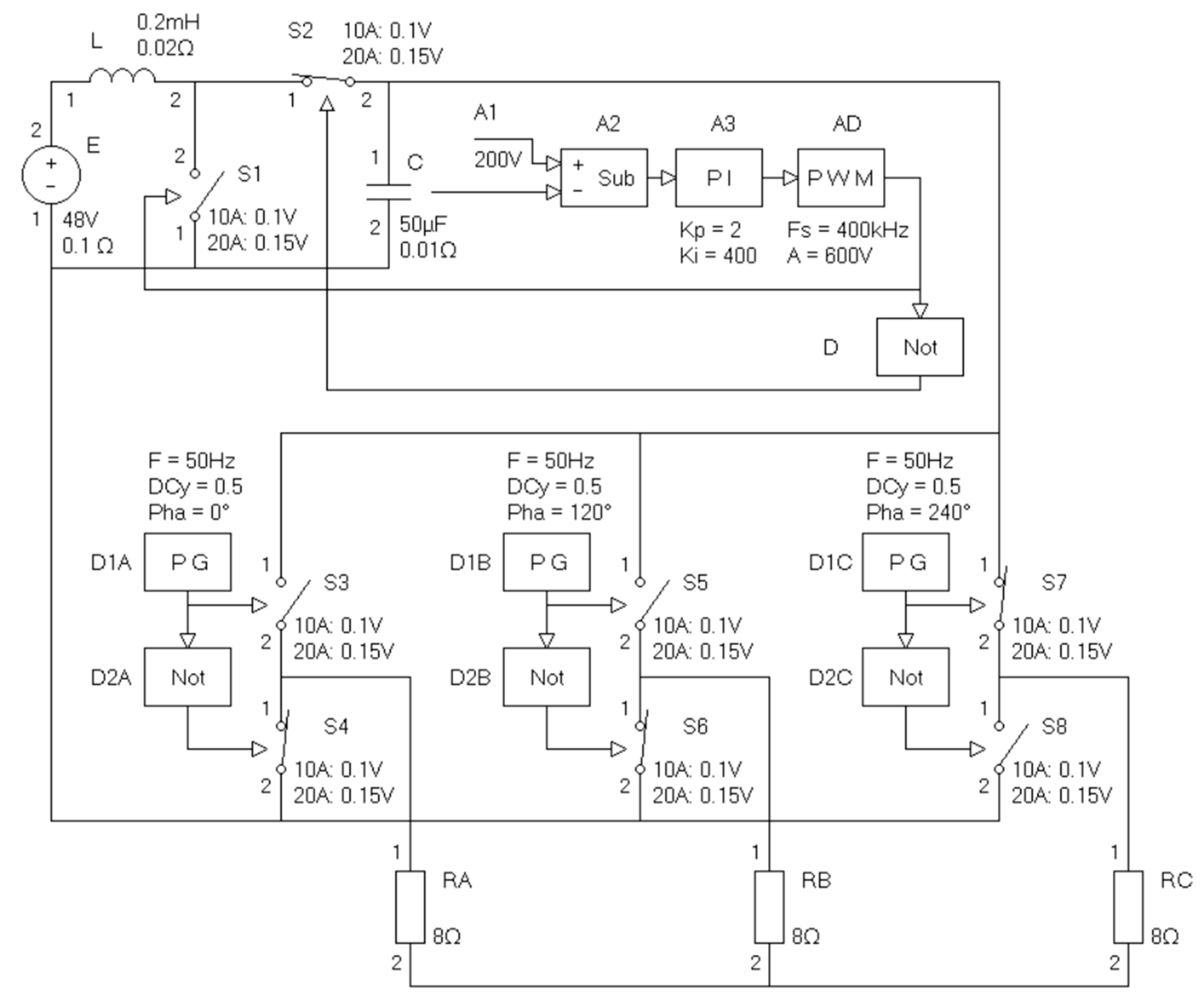
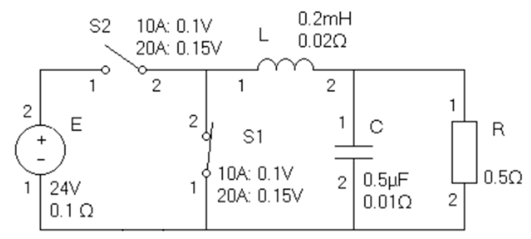
2.3. R-IM Models of Electronic Components, Circuits and Devices

Let an electronic device be modelled and be denoted by D, and let ${\mathrm{M}}_{\mathrm{D}}$ be a finite set of unique indices associated to its components. It is obvious that various divisions can be performed in non-trivial devices, and appropriate hierarchies, which include sub-devices, can be defined. In [12] a two-terminal electronic component ${\mathrm{c}}_{\mathrm{m}}$, $\mathrm{m}\in {\mathrm{M}}_{\mathrm{D}},$ is modelled by R-IM ${\overline{\mathrm{F}}}_{\mathrm{m}}(\mathrm{t})$ so that a relation between its voltages ${\mathrm{u}}_{\mathrm{m}}(\mathrm{t}),$ ${\mathrm{u}}_{\mathrm{m}}(\mathrm{t}-\Delta \mathrm{t})$ and its amperages ${\mathrm{i}}_{\mathrm{m}}(\mathrm{t}),$ ${\mathrm{i}}_{\mathrm{m}}(\mathrm{t}-\Delta \mathrm{t})$ at consecutive time moments can be obtained (respective indices ${\mathrm{u}}_{\mathrm{m}}^{\mathrm{c}\mathrm{u}}$, ${\mathrm{u}}_{\mathrm{m}}^{\mathrm{p}\mathrm{r}}$, ${\mathrm{i}}_{\mathrm{m}}^{\mathrm{c}\mathrm{u}}$ and ${\mathrm{i}}_{\mathrm{m}}^{\mathrm{p}\mathrm{r}}$, which do not depend on time, are used); here $\mathrm{t}\in \mathrm{\Theta }-{\mathrm{t}}_0$. This relation is given by

$${\overline{\mathrm{F}}}_{\mathrm{m}}(\mathrm{t}) \odot {\overline{{\mathrm{X}}^{″}}}_{\mathrm{m}}(\mathrm{t})=\overline{\mathrm{O}},\hspace{1em}\hspace{1em}{\mathrm{I}}_2\left({\overline{\mathrm{F}}}_{\mathrm{m}}(\mathrm{t})\right)\equiv {\mathrm{I}}_1\left({\overline{{\mathrm{X}}^{″}}}_{\mathrm{m}}(\mathrm{t})\right).$$

(22)

Both values and their respective indices are presented in ${\overline{{\mathrm{X}}^{″}}}_{\mathrm{m}}(\mathrm{t})$ (see (24)). Here and below $\overline{\mathrm{O}}$ denotes a zero R-IM (all its elements are zeros). Examples on basic components are given in [12] and below.

Let an electronic component, denoted by ${\mathrm{c}}_{\mathrm{L}}$, be an inductor with inductance $\mathrm{L}$. Approximation

$${\mathrm{u}}_{\mathrm{L}}(\mathrm{t})=\mathrm{L}\frac{{\mathrm{i}}_{\mathrm{L}}(\mathrm{t})-{\mathrm{i}}_{\mathrm{L}}(\mathrm{t}-\Delta \mathrm{t})}{\Delta \mathrm{t}}$$

(23)

is a consequence of

$${\overline{\mathrm{F}}}_{\mathrm{L}} \odot \begin{array}{ll}\underset{\_}{{}_{}}\hfill & \underset{\_}{|\mathrm{o}}\hfill \\ {\mathrm{u}}_{\mathrm{L}}^{\mathrm{c}\mathrm{u}}\hfill & |{\mathrm{u}}_{\mathrm{L}}(\mathrm{t})\hfill \\ {\mathrm{i}}_{\mathrm{L}}^{\mathrm{c}\mathrm{u}}\hfill & |{\mathrm{i}}_{\mathrm{L}}(\mathrm{t})\hfill \\ {\mathrm{i}}_{\mathrm{L}}^{\mathrm{p}\mathrm{r}}\hfill & |{\mathrm{i}}_{\mathrm{L}}(\mathrm{t}-\Delta \mathrm{t})\hfill \end{array}=\mathrm{O},\hspace{1em}\hspace{1em}{\overline{\mathrm{F}}}_{\mathrm{L}}=\begin{array}{cccc}\underset{\_}{}& \underset{\_}{|{\mathrm{u}}_{\mathrm{L}}^{\mathrm{c}\mathrm{u}}}\hfill & \underset{\_}{{\mathrm{i}}_{\mathrm{L}}^{\mathrm{c}\mathrm{u}}}& \underset{\_}{{\mathrm{i}}_{\mathrm{L}}^{\mathrm{p}\mathrm{r}}}\\ {\mathrm{c}}_{\mathrm{L}}& |\begin{array}{c}\\ \end{array}1\hfill & -\frac{\mathrm{L}}{\Delta \mathrm{t}}& \frac{\mathrm{L}}{\Delta \mathrm{t}}\end{array}$$

(24)

Similarly, for a capacitor, denoted by ${\mathrm{c}}_{\mathrm{C}}$, with capacitance C,

$${\overline{\mathrm{F}}}_{\mathrm{C}}=\begin{array}{cccc}\underset{\_}{}& \underset{\_}{|{\mathrm{u}}_{\mathrm{C}}^{\mathrm{c}\mathrm{u}}}\hfill & \underset{\_}{{\mathrm{i}}_{\mathrm{C}}^{\mathrm{c}\mathrm{u}}}& \underset{\_}{{\mathrm{u}}_{\mathrm{C}}^{\mathrm{p}\mathrm{r}}}\\ {\mathrm{c}}_{\mathrm{C}}& |\begin{array}{c}\\ \end{array}-\frac{\mathrm{C}}{\Delta \mathrm{t}}\hfill & 1& \frac{\mathrm{C}}{\Delta \mathrm{t}}\end{array}$$

(25)

gives approximation

$${\mathrm{i}}_{\mathrm{C}}(\mathrm{t})=\mathrm{C}\frac{{\mathrm{u}}_{\mathrm{C}}(\mathrm{t})-{\mathrm{u}}_{\mathrm{C}}(\mathrm{t}-\Delta \mathrm{t})}{\Delta \mathrm{t}}.$$

(26)

It is obvious that (5) models a resistor, denoted by ${\mathrm{c}}_{\mathrm{R}}$, with resistance R. For an ideal DC voltage source, denoted by ${\mathrm{c}}_{\mathrm{E}}$, constant voltage $\mathrm{E}$ is determined by

$${\overline{\mathrm{F}}}_{\mathrm{E}} \odot \begin{array}{cc}\underset{\_}{}& \underset{\_}{|\mathrm{o}}\hfill \\ {\mathrm{u}}_{\mathrm{E}}^{\mathrm{c}\mathrm{u}}& |{\mathrm{u}}_{\mathrm{E}}^{}\left(\mathrm{t}\right)\hfill \\ \mathrm{o}& |1\hfill \end{array}=\mathrm{O},\hspace{1em}\hspace{1em}{\overline{\mathrm{F}}}_{\mathrm{E}}=\begin{array}{ccc}{}_{\underset{\_}{}}^{}& \underset{\_}{|{\mathrm{u}}_{\mathrm{E}}^{\mathrm{c}\mathrm{u}}}\hfill & \underset{\_}{\mathrm{o}}\\ {\mathrm{c}}_{\mathrm{E}}& |1\hfill & \mathrm{E}\end{array}.$$

(27)

The upper parameters L, C, R and E, do not depend on time. However, their time dependences can be presented instead of constants. Let the component, denoted by ${\mathrm{c}}_{\mathrm{S}}$, be an ideal electronic switch; a joint representation of its two states is

$${\overline{\mathrm{F}}}_{\mathrm{S}}(\mathrm{t})=\begin{array}{ccc}{}_{\underset{\_}{}}^{}& \underset{\_}{|{\mathrm{u}}_{\mathrm{S}}^{\mathrm{c}\mathrm{u}} }\hfill & \underset{\_}{{\mathrm{i}}_{\mathrm{S}}^{\mathrm{c}\mathrm{u}}}\\ {\mathrm{c}}_{\mathrm{S}}& |{\mathrm{s}}_{\mathrm{S}}(\mathrm{t})\hfill & 1-{\mathrm{s}}_{\mathrm{S}}(\mathrm{t})\end{array},$$

(28)

where ${\mathrm{s}}_{\mathrm{S}}:\mathrm{\Theta }\to \left\{0;1\right\}$ is a switching function. According to (28), in the closed state of the switch ${\mathrm{u}}_{\mathrm{S}}(\mathrm{t})=0,$ and in its opened state ${\mathrm{i}}_{\mathrm{S}}(\mathrm{t})=0.$

Nodes are modeled by IMs below according to Kirchhoff’s current law in a similar manner. Each component index in the left side of the next three equations denotes an electronic component which is not presented in previous such equations. For the scheme with two-terminal components from Figure 1 the respective R-IMs are

$${\overline{\mathrm{F}}}_{{\mathrm{n}}_{\mathrm{E}}}=\begin{array}{ccc}\underset{\_}{}& \underset{\_}{|{\mathrm{i}}_{{\mathrm{E}}_{{}_{}}}^{\mathrm{c}\mathrm{u}}}\hfill & \underset{\_}{{\mathrm{i}}_{{\mathrm{S}}_2}^{\mathrm{c}\mathrm{u}}}\\ {\mathrm{n}}_{\mathrm{E}}& |1\hfill & -1\end{array};\hspace{1em}\hspace{1em}{\overline{\mathrm{F}}}_{{\mathrm{n}}_{{\mathrm{S}}_2}}=\begin{array}{cccc}\underset{\_}{}& \underset{\_}{|{\mathrm{i}}_{{\mathrm{S}}_2}^{\mathrm{c}\mathrm{u}}}\hfill & \underset{\_}{{\mathrm{i}}_{{\mathrm{S}}_1}^{\mathrm{c}\mathrm{u}}}& \underset{\_}{{\mathrm{i}}_{{\mathrm{L}}_{{}_{}}}^{\mathrm{c}\mathrm{u}}}\\ {\mathrm{n}}_{{\mathrm{S}}_2}& |1\hfill & 1& -1\end{array};\hspace{1em}\hspace{1em}{\overline{\mathrm{F}}}_{{\mathrm{n}}_{\mathrm{L}}}=\begin{array}{cccc}\underset{\_}{}& \underset{\_}{|{\mathrm{i}}_{\mathrm{L}}^{\mathrm{c}\mathrm{u}}}\hfill & \underset{\_}{{\mathrm{i}}_{\mathrm{C}}^{\mathrm{c}\mathrm{u}}}& \underset{\_}{{\mathrm{i}}_{\mathrm{R}}^{\mathrm{c}\mathrm{u}}}\\ {\mathrm{n}}_{\mathrm{L}}& |1\hfill & -1& -1\end{array} .$$

(29)

They model

$${\mathrm{i}}_{\mathrm{E}}^{}\left(\mathrm{t}\right)-{\mathrm{i}}_{{\mathrm{S}}_2}^{}\left(\mathrm{t}\right)=0;\hspace{1em}\hspace{1em}{\mathrm{i}}_{{\mathrm{S}}_2}^{}\left(\mathrm{t}\right)+{\mathrm{i}}_{{\mathrm{S}}_1}^{}\left(\mathrm{t}\right)-{\mathrm{i}}_{\mathrm{L}}^{}\left(\mathrm{t}\right)=0;\hspace{1em}\hspace{1em}{\mathrm{i}}_{\mathrm{L}}^{}\left(\mathrm{t}\right)-{\mathrm{i}}_{\mathrm{C}}^{}\left(\mathrm{t}\right)-{\mathrm{i}}_{\mathrm{R}}^{}\left(\mathrm{t}\right)=0.$$

(30)

The R-IM on the fourth node is omitted, because it gives a linear combination of R-IMs from (29); all elements of ${\mathrm{M}}_{\mathrm{C}\mathrm{i}\mathrm{r}\mathrm{c}}=\left\{“\mathrm{E}”; “{\mathrm{S}}_2”; “{\mathrm{S}}_1”; “\mathrm{L}”; “\mathrm{C}”; “\mathrm{R}”\right\}$ are represented in these three R-IMs (the circuit is denoted by “Circ”). For each component, the positive direction of voltage and amperage is from its first to its second terminal, and it determines respective signs in the index matrices from (29) and (31).

Kirchhoff’s voltage law can be applied through index matrices too. For the scheme from Figure 1, respective R-IMs on three loops are

$${\overline{\mathrm{F}}}_{{\mathrm{p}}_{\mathrm{R}}}=\begin{array}{ccc}\underset{\_}{}& \underset{\_}{|{\mathrm{u}}_{\mathrm{R}}^{\mathrm{c}\mathrm{u}}}\hfill & \underset{\_}{{\mathrm{u}}_{\mathrm{C}}^{\mathrm{c}\mathrm{u}}}\\ {\mathrm{p}}_{\mathrm{R}}& |1\hfill & -1\end{array};\hspace{1em}\hspace{1em}{\overline{\mathrm{F}}}_{{\mathrm{p}}_{\mathrm{E}}}=\begin{array}{cccc}\underset{\_}{}& \underset{\_}{|{\mathrm{u}}_{\mathrm{E}}^{\mathrm{c}\mathrm{u}}}\hfill & \underset{\_}{{\mathrm{u}}_{{\mathrm{S}}_2}^{\mathrm{c}\mathrm{u}}}& \underset{\_}{{\mathrm{u}}_{{\mathrm{S}}_1}^{\mathrm{c}\mathrm{u}}}\\ {\mathrm{p}}_{\mathrm{E}}& |1\hfill & 1& -1\end{array};\hspace{1em}\hspace{1em}{\overline{\mathrm{F}}}_{{\mathrm{p}}_{\mathrm{L}}}=\begin{array}{cccc}\underset{\_}{}& \underset{\_}{|{\mathrm{u}}_{\mathrm{L}}^{\mathrm{c}\mathrm{u}}}\hfill & \underset{\_}{{\mathrm{u}}_{\mathrm{C}}^{\mathrm{c}\mathrm{u}}}& \underset{\_}{{\mathrm{u}}_{{\mathrm{S}}_1}^{\mathrm{c}\mathrm{u}}}\\ {\mathrm{p}}_{\mathrm{L}}& |1\hfill & 1& 1\end{array}.$$

(31)

They model

$${\mathrm{u}}_{\mathrm{R}}^{}\left(\mathrm{t}\right)-{\mathrm{u}}_{\mathrm{C}}^{}\left(\mathrm{t}\right)=0;\hspace{1em}{\mathrm{u}}_{\mathrm{E}}^{}\left(\mathrm{t}\right)+{\mathrm{u}}_{{\mathrm{S}}_2}^{}\left(\mathrm{t}\right)-{\mathrm{u}}_{{\mathrm{S}}_1}^{}\left(\mathrm{t}\right)=0;\hspace{1em}{\mathrm{u}}_{\mathrm{L}}^{}\left(\mathrm{t}\right)+{\mathrm{u}}_{\mathrm{C}}^{}\left(\mathrm{t}\right)+{\mathrm{u}}_{{\mathrm{S}}_1}^{}\left(\mathrm{t}\right)=0.$$

(32)

For the considered circuit, denoted by “Circ”, statements

$${\overline{\mathrm{F}}}_{\mathrm{C}\mathrm{i}\mathrm{r}\mathrm{c}}(\mathrm{t})=\left(\underset{\mathrm{m}{\in }^{{}^{}}{\mathrm{M}}_{\mathrm{C}\mathrm{i}\mathrm{r}\mathrm{c}}}{\oplus }{\overline{\mathrm{F}}}_{\mathrm{m}}(\mathrm{t})\right)\oplus \left(\underset{\mathrm{n}{\in }^{{}^{}}{\mathrm{N}}_{\mathrm{C}\mathrm{i}\mathrm{r}\mathrm{c}}}{\oplus }{\overline{\mathrm{F}}}_{\mathrm{n}}\right)\oplus \left(\underset{\mathrm{p}{\in }^{{}^{}}{\mathrm{P}}_{\mathrm{C}\mathrm{i}\mathrm{r}\mathrm{c}}}{\oplus }{\overline{\mathrm{F}}}_{\mathrm{p}}\right);$$

(33)

$$\underset{\mathrm{m}{\in }^{{}^{{}^{}}}{\mathrm{M}}_{\mathrm{C}\mathrm{i}\mathrm{r}\mathrm{c}}}{\oplus }{\overline{\mathrm{F}}}_{\mathrm{m}}\left(\mathrm{t}\right)={\overline{\mathrm{F}}}_{Е}(\mathrm{t})\oplus {\overline{\mathrm{F}}}_{{\mathrm{S}}_1}(\mathrm{t})\oplus {\overline{\mathrm{F}}}_{{\mathrm{S}}_2}(\mathrm{t})\oplus {\overline{\mathrm{F}}}_{\mathrm{L}}\oplus {\overline{\mathrm{F}}}_{\mathrm{C}}\oplus {\overline{\mathrm{F}}}_{\mathrm{R}};$$

(34)

$$\underset{\mathrm{n}{\in }^{{}^{}}{\mathrm{N}}_{\mathrm{C}\mathrm{i}\mathrm{r}\mathrm{c}}}{\oplus }{\overline{\mathrm{F}}}_{\mathrm{n}}={\overline{\mathrm{F}}}_{{\mathrm{n}}_{\mathrm{E}}}\oplus {\overline{\mathrm{F}}}_{{\mathrm{n}}_{{\mathrm{S}}_2}} \oplus {\overline{\mathrm{F}}}_{{\mathrm{n}}_{\mathrm{L}}};\hspace{1em}\hspace{1em}\underset{\mathrm{p}{\in }^{{}^{}}{\mathrm{P}}_{\mathrm{C}\mathrm{i}\mathrm{r}\mathrm{c}}}{\oplus }{\overline{\mathrm{F}}}_{\mathrm{p}}={\overline{\mathrm{F}}}_{{\mathrm{p}}_{\mathrm{R}}}\oplus {\overline{\mathrm{F}}}_{{\mathrm{p}}_{\mathrm{E}}}\oplus {\overline{\mathrm{F}}}_{{\mathrm{p}}_{\mathrm{L}}}.$$

(35)

combine models of components, nodes, and loops. Sparse R-IM ${\overline{\mathrm{F}}}_{\mathrm{C}\mathrm{i}\mathrm{r}\mathrm{c}}\left(\mathrm{t}\right)$ contains 12 columns, which have indices with subscript “cu”, and 12 rows. It is a part of a bigger model in the present paper. Resistances are associated to the inductor, the capacitor, the DC voltage source and the switches (voltages on closed switches are juxtaposed to amperages), and therefore ${\overline{\mathrm{F}}}_{\mathrm{L}}$, ${\overline{\mathrm{F}}}_{\mathrm{C}}$, ${\overline{\mathrm{F}}}_{\mathrm{E}}$, ${\overline{\mathrm{F}}}_{{\mathrm{S}}_1}(\mathrm{t})$ and ${\overline{\mathrm{F}}}_{{\mathrm{S}}_2}(\mathrm{t})$ are modified. Devices, which are connected to the upper circuit, are depicted in Figure 2 and described below. Their circuits are not considered; only important inputs and outputs are taken into account and shown graphically; voltages on all devices are denoted in the figures. The digital signals are denoted by “s”. The considered buck converter uses five blocks: a constant voltage block, a subtraction block, a proportional-integral (PI) controller, a pulse width modulation (PWM) block, and a logical NOT gate.

The constant voltage block is represented by

$${\overline{\mathrm{F}}}_{\mathrm{A}1}=\begin{array}{ccc}\underset{\_}{}& \underset{\_}{|{\mathrm{u}}_{\mathrm{A}1}^{\mathrm{c}\mathrm{u}}}& \underset{\_}{{\mathrm{u}}_{\mathrm{A}1,1}^{\mathrm{c}\mathrm{u}}}\\ {\mathrm{c}}_{\mathrm{A}1}& |-1& \mathrm{U}\end{array}.$$

(36)

All input and output signals are marked by the respective component names, and the input ones are numbered. In the shown example $\mathrm{U}=10\mathrm{V}.$

The subtraction block is represented by

$${\overline{\mathrm{F}}}_{\mathrm{A}2}=\begin{array}{cccc}\underset{\_}{}& \underset{\_}{|{\mathrm{u}}_{\mathrm{A}2}^{\mathrm{c}\mathrm{u}}}& \underset{\_}{{\mathrm{u}}_{\mathrm{A}2,1}^{\mathrm{c}\mathrm{u}}}& \underset{\_}{{\mathrm{u}}_{\mathrm{A}2,2}^{\mathrm{c}\mathrm{u}}}\\ {\mathrm{c}}_{\mathrm{A}2}& |-1& 1& -1\end{array}.$$

(37)

The proportional-integral (PI) controller is modeled by

$${\overline{\mathrm{F}}}_{\mathrm{A}3}=\begin{array}{lllll}\underset{\_}{}\hfill & \underset{\_}{|{\mathrm{u}}_{\mathrm{A}3}^{\mathrm{c}\mathrm{u}} }\hfill & \underset{\_}{{\mathrm{u}}_{\mathrm{A}3}^{\mathrm{p}\mathrm{r}}}\hfill & \underset{\_}{{\mathrm{u}}_{\mathrm{A}3,1}^{\mathrm{c}\mathrm{u}}}\hfill & \underset{\_}{{\mathrm{u}}_{\mathrm{A}3,1}^{\mathrm{p}\mathrm{r}} }\hfill \\ {\mathrm{c}}_{\mathrm{A}3}\hfill & |\begin{array}{c}\\ \end{array}-\frac{1}{\Delta \mathrm{t}}\hfill & \frac{1}{\Delta \mathrm{t}}\hfill & \frac{{\mathrm{K}}_{\mathrm{p}}}{\Delta \mathrm{t}}+{\mathrm{K}}_{\mathrm{i}}\hfill & -\frac{{\mathrm{K}}_{\mathrm{p}}}{\Delta \mathrm{t}}\hfill \end{array} .$$

(38)

The last index matrix approximates

$$\frac{\mathrm{d}{\mathrm{u}}_{\mathrm{A}3}(\mathrm{t})}{\mathrm{d}\mathrm{t}}={\mathrm{K}}_{\mathrm{p}}\frac{\mathrm{d}{\mathrm{u}}_{\mathrm{A}3,1}(\mathrm{t})}{\mathrm{d}\mathrm{t}}+{\mathrm{K}}_{\mathrm{i}}{\mathrm{u}}_{\mathrm{A}3,1}(\mathrm{t}),$$

(39)

which is obtained from basic definition

$${\mathrm{u}}_{\mathrm{A}3}(\mathrm{t})={\mathrm{K}}_{\mathrm{p}}{\mathrm{u}}_{\mathrm{A}3,1}(\mathrm{t})+{\mathrm{K}}_{\mathrm{i}}{\displaystyle {\int }_0^{\mathrm{t}} {\mathrm{u}}_{\mathrm{A}3,1}(\mathsf{\theta })}\mathrm{d}\mathsf{\theta }$$

(40)

via differentiation. Proper values of ${\mathrm{K}}_{\mathrm{p}}$ and ${\mathrm{K}}_{\mathrm{i}}$ are shown in Figure 2.

The PWM block is modeled by

$${\overline{\mathrm{F}}}_{\mathrm{A}\mathrm{D}}(\mathrm{t})=\{\begin{array}{cc}\begin{array}{lll}\underset{\_}{}\hfill & \underset{\_}{|{\mathrm{s}}_{\mathrm{A}\mathrm{D}}^{\mathrm{c}\mathrm{u}}}\hfill & \underset{\_}{\mathrm{o}}\hfill \\ {\mathrm{c}}_{\mathrm{A}\mathrm{D}}\hfill & |-1_{}\hfill & 1\hfill \end{array},& \mathrm{i}\mathrm{f}\hspace{1em}{\mathrm{u}}_{\mathrm{A}\mathrm{D},1}({\mathrm{t}}_{\mathrm{s}})>{\mathrm{u}}_{\mathrm{T}\mathrm{r}\mathrm{i}\mathrm{a}\mathrm{n}\mathrm{g}}(\mathrm{t}-\Delta \mathrm{t});\\ \begin{array}{cc}\underset{\_}{}& \underset{\_}{|{\mathrm{s}}_{\mathrm{A}\mathrm{D}}^{\mathrm{c}\mathrm{u}}}\\ {\mathrm{c}}_{\mathrm{A}\mathrm{D}}& |-1\end{array},& \mathrm{o}\mathrm{t}\mathrm{h}\mathrm{e}\mathrm{r}\mathrm{w}\mathrm{i}\mathrm{s}\mathrm{e};\end{array}$$

(41)

where

$${\mathrm{t}}_{\mathrm{s}}=\left\{\begin{array}{ccccc}0,& \pm \Delta {\mathrm{t}}_{\mathrm{s}},& \pm 2\Delta {\mathrm{t}}_{\mathrm{s}},& \pm 3\Delta {\mathrm{t}}_{\mathrm{s}},& \dots \end{array}\right\}\cap (\mathrm{t}-\Delta \mathrm{t}-\Delta {\mathrm{t}}_{\mathrm{s}},\mathrm{t}-\Delta \mathrm{t}] .$$

(42)

Here the signal

$${\mathrm{u}}_{\mathrm{T}\mathrm{r}\mathrm{i}\mathrm{a}\mathrm{n}\mathrm{g}}:\mathrm{\Theta } \to \left[0,\mathrm{A}\right]$$

(43)

has a triangular form, period $\Delta {\mathrm{t}}_{\mathrm{s}}=\frac{1}{{\mathrm{F}}_{\mathrm{s}}}$ and amplitude $\mathrm{A}$. Тhe output of the PI controller is checked with switching frequency ${\mathrm{F}}_{\mathrm{s}}$. The voltage on the output of the PI controller and the triangular function forms a duty cycle. The last two index matrices represent alternatives ${\mathrm{s}}_{\mathrm{A}\mathrm{D}}(\mathrm{t})=1$ and ${\mathrm{s}}_{\mathrm{A}\mathrm{D}}(\mathrm{t})=0$, i.e., they form a digital signal. Proper values of ${\mathrm{F}}_{\mathrm{s}}$ and A are shown in Figure 2.

Finally, the logical NOT gate is modeled by

$${\overline{\mathrm{F}}}_{\mathrm{D}}=\begin{array}{cccc}\underset{\_}{}& \underset{\_}{|{\mathrm{s}}_{\mathrm{D}}^{\mathrm{c}\mathrm{u}}}\hfill & \underset{\_}{{\mathrm{s}}_{\mathrm{D},1}^{\mathrm{c}\mathrm{u}}}& \underset{\_}{{\mathrm{o}}_{}}\\ {\mathrm{c}}_{\mathrm{D}}& |-1\hfill & -1& 1\end{array} ,$$

(44)

Values ${\mathrm{s}}_{\mathrm{I}\mathrm{n}v,1}(\mathrm{t})$ and ${\mathrm{s}}_{\mathrm{I}\mathrm{n}v}(\mathrm{t})$ belong to set $\left\{0,1\right\}$ too.

All junctions of the considered five blocks are represented by

$$\begin{array}{lll}\underset{\_}{}\hfill & \underset{\_}{|{\mathrm{u}}_{\mathrm{A}2,1}^{\mathrm{c}\mathrm{u}}}\hfill & \underset{\_}{{\mathrm{u}}_{\mathrm{A}{1}_{}}^{\mathrm{c}\mathrm{u}}}\hfill \\ {\mathrm{p}}_{\mathrm{A}2,1}\hfill & |-1\hfill & 1\hfill \end{array} ;\hspace{1em}\begin{array}{lll}\underset{\_}{}\hfill & \underset{\_}{|{\mathrm{u}}_{\mathrm{A}2,2}^{\mathrm{c}\mathrm{u}}}\hfill & \underset{\_}{{\mathrm{u}}_{{\mathrm{R}}_{}}^{\mathrm{c}\mathrm{u}}}\hfill \\ {\mathrm{p}}_{\mathrm{A}2,2}\hfill & |-1\hfill & 1\hfill \end{array} ;\hspace{1em}\begin{array}{lll}\underset{\_}{}\hfill & \underset{\_}{|{\mathrm{u}}_{\mathrm{A}3,1}^{\mathrm{c}\mathrm{u}}}\hfill & \underset{\_}{{\mathrm{u}}_{\mathrm{A}{2}_{}}^{\mathrm{c}\mathrm{u}}}\hfill \\ {\mathrm{p}}_{\mathrm{A}3,1}\hfill & |-1\hfill & 1\hfill \end{array} ;\hspace{1em}\begin{array}{lll}\underset{\_}{}\hfill & \underset{\_}{|{\mathrm{u}}_{\mathrm{A}\mathrm{D},1}^{\mathrm{c}\mathrm{u}}}\hfill & \underset{\_}{{\mathrm{u}}_{\mathrm{A}{3}_{}}^{\mathrm{c}\mathrm{u}}}\hfill \\ {\mathrm{p}}_{\mathrm{A}\mathrm{D},1}\hfill & |-1\hfill & 1\hfill \end{array} ;$$

$$\begin{array}{lll}\underset{\_}{}\hfill & \underset{\_}{|{\mathrm{s}}_{\mathrm{D},1}^{\mathrm{c}\mathrm{u}}}\hfill & \underset{\_}{{\mathrm{s}}_{\mathrm{A}{\mathrm{D}}_{}}^{\mathrm{c}\mathrm{u}}}\hfill \\ {\mathrm{p}}_{\mathrm{D},1}\hfill & |-1\hfill & 1\hfill \end{array};\hspace{1em}\hspace{1em}\begin{array}{lll}\underset{\_}{}\hfill & \underset{\_}{|{\mathrm{s}}_{{\mathrm{S}}_1}^{\mathrm{c}\mathrm{u}}}\hfill & \underset{\_}{{\mathrm{s}}_{\mathrm{A}{\mathrm{D}}_{{}_{}}}^{\mathrm{c}\mathrm{u}}}\hfill \\ {\mathrm{p}}_{{\mathrm{S}}_1,1}\hfill & |-1\hfill & 1\hfill \end{array};\hspace{1em}\hspace{1em}\begin{array}{lll}\underset{\_}{{}_{{}_{{}_{{}_{{}_{{}_{}}}}}}}\hfill & \underset{\_}{|{\mathrm{s}}_{{\mathrm{S}}_2}^{\mathrm{c}\mathrm{u}}}\hfill & \underset{\_}{{\mathrm{s}}_{{\mathrm{D}}_{{}_{}}}^{\mathrm{c}\mathrm{u}}}\hfill \\ {\mathrm{p}}_{{\mathrm{S}}_2,1}\hfill & |-1\hfill & 1\hfill \end{array}.$$

(45)

The last two index matrices determine values of the switching functions.

The controller (denoted by “Contr” below) can be modeled by

$${\overline{\mathrm{F}}}_{\mathrm{C}\mathrm{o}\mathrm{n}\mathrm{t}\mathrm{r}}(\mathrm{t})=\left({\overline{\mathrm{F}}}_{\mathrm{A}1}\oplus {\overline{\mathrm{F}}}_{\mathrm{A}2}\oplus {\overline{\mathrm{F}}}_{\mathrm{A}2}\oplus {\overline{\mathrm{F}}}_{\mathrm{A}\mathrm{D}}(\mathrm{t})\oplus {\overline{\mathrm{F}}}_{\mathrm{D}}\right)\oplus {\overline{\mathrm{F}}}_{{\mathrm{P}}_{\mathrm{C}\mathrm{o}\mathrm{n}\mathrm{r}}},$$

(46)

where the last index matrix is calculated as a sum of the R-IMs in (45). A common model (denoted by “Buck Conv”) is

$${\overline{\mathrm{F}}}_{\mathrm{B}\mathrm{u}\mathrm{c}\mathrm{k}\mathrm{C}\mathrm{o}\mathrm{n}v}(\mathrm{t})={\overline{\mathrm{F}}}_{\mathrm{C}\mathrm{i}\mathrm{r}\mathrm{c}}(\mathrm{t})\oplus {\overline{\mathrm{F}}}_{\mathrm{C}\mathrm{o}\mathrm{n}\mathrm{t}\mathrm{r}}(\mathrm{t}).$$

(47)

A relation between voltages and amperages can be obtained through R-IM equation

$${\overline{\mathrm{F}}}_{\mathrm{B}\mathrm{u}\mathrm{c}\mathrm{k}\mathrm{C}\mathrm{o}\mathrm{n}\mathrm{v}}(\mathrm{t})\odot {\overline{{\mathrm{X}}^{″}}}_{\mathrm{B}\mathrm{u}\mathrm{c}\mathrm{k}\mathrm{C}\mathrm{o}\mathrm{n}\mathrm{v}}(\mathrm{t})=\overline{\mathrm{O}},\hspace{1em}{\mathrm{I}}_2\left({\overline{\mathrm{F}}}_{\mathrm{B}\mathrm{u}\mathrm{c}\mathrm{k}\mathrm{C}\mathrm{o}\mathrm{n}\mathrm{v}}(\mathrm{t})\right)\equiv {\mathrm{I}}_1\left({\overline{{\mathrm{X}}^{″}}}_{\mathrm{B}\mathrm{u}\mathrm{c}\mathrm{k}\mathrm{C}\mathrm{o}\mathrm{n}\mathrm{v}}(\mathrm{t})\right),$$

(48)

where both values and their respective indices are presented in ${\overline{{\mathrm{X}}^{″}}}_{\mathrm{B}\mathrm{u}\mathrm{c}\mathrm{k}\mathrm{C}\mathrm{o}\mathrm{n}\mathrm{v}}(\mathrm{t})$.

The equation in (48) is a proper R-IM analog of the matrix equation in (21), i.e., it represents a first-order discrete dynamical system. Sparse R-IM ${\overline{\mathrm{F}}}_{\mathrm{B}\mathrm{u}\mathrm{c}\mathrm{k}\mathrm{C}\mathrm{o}\mathrm{n}\mathrm{v}}(\mathrm{t})$ contains 24 columns, which have indices with subscript “cu”, and 24 rows (there are 12 R-IMs in ${\overline{\mathrm{F}}}_{\mathrm{C}\mathrm{o}\mathrm{n}\mathrm{t}\mathrm{r}}\left(\mathrm{t}\right)$ with 12 indices with subscript “cu”, which are not presented in ${\overline{\mathrm{F}}}_{\mathrm{C}\mathrm{i}\mathrm{r}\mathrm{c}}\left(\mathrm{t}\right))$. All R-IM models in the present section are automatically simplified (since the index matrices in (45) are trivial, all 24 respective variables are automatically reduced to 15 analog ones and 4 discrete ones), generated and solved by the software, which is developed by the authors (see next section).

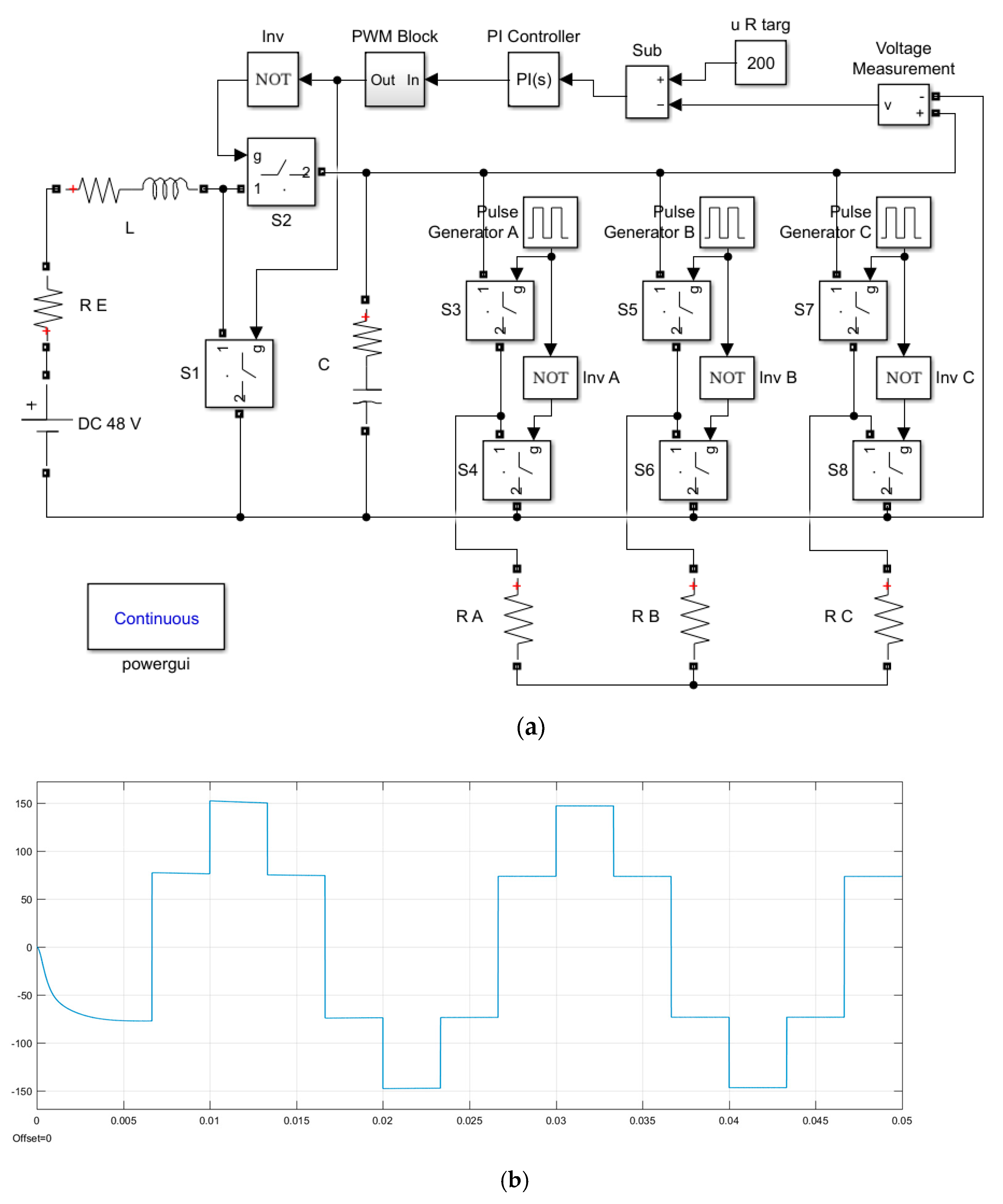
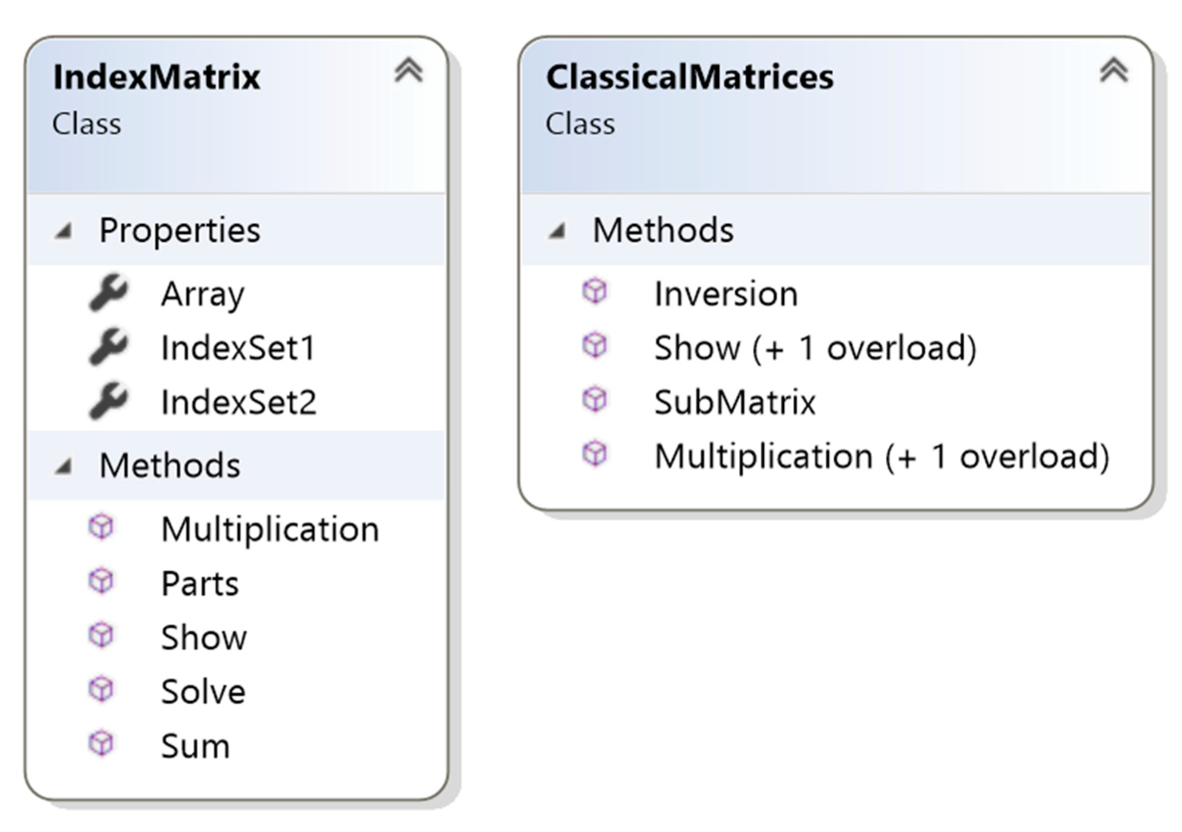
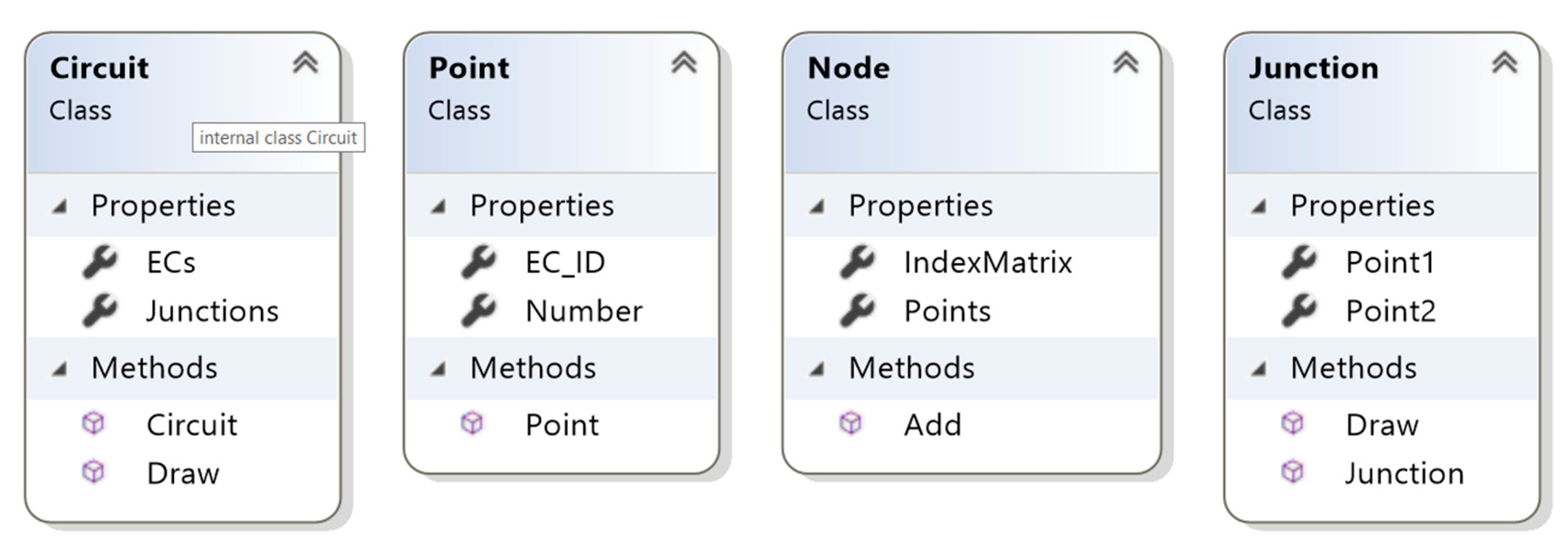
3. Software Implementation Based on R-IMs

In [5], programming classes, which implement electronic circuit design techniques, and which are based on R-IMs, are presented. Class diagrams of their recent versions are shown in this section. One of the main purposes is the automation of processes of modeling and simulation. An example of joint modeling and simulation of a power circuit and a PI controller is given. All electronic component images in the present paper, except the ones which use Simulink, are obtained by labeling the authors’ methods as Draw().

Each object of class IndexMatrix represents a R-IM through two lists of indices and a two-dimensional array. Static methods Sum() and Multiplication() implement the operations, which are considered in (7) and (11). The method Solve() transforms a R-IM analog of discrete dynamical system model (21) (see (48)) to a R-IM analog of equation (20) in order that state variables can be calculated in a step-wise manner at each simulation step. In this process, the auxiliary method Parts() is used in distinguishing current values from previous ones. Class ClassicalMatrices contain static methods, which implement well-known operations over classical matrixes (multiplication, inversion, and calculation of the sub-matrix), which are used in model solving. Class diagrams of IndexMatrix and ClassicalMatrices are presented in Figure 3.

Class EC and its subclasses for the considered electronic components are presented in Figure 4. Various specific properties (L, C, R, E, Ki, Kp, etc.) are defined. The method CalculateIM() forms RI-Ms according to the statements, which are given in the paper. The common properties of Position, Rotation and ConnectionPositions are used in drawing (method Draw() is overridden). The members of interfaces, which are used in subclasses of EC, are shown in Figure 4 too.

Class diagrams of Circuit and its auxiliary classes are shown in Figure 5. Each object of class Junction represents a connection between two electronic components, and each object of class Node implements a connection (such as the ones modeled in (29)) between two or more components. Finally, class Circuit defines collections of instances of types EC and Junction.

Class Simlation determines in each instance an electronic circuit, a discretization frequency, and a model time interval. Its method Do() invokes private methods in order for proper R-IMs to be constructed and handled; notes on these methods and results of their functioning in case of the considered example are given below:

CalculateConstantIMOnComponents(): performs in field IMAnalog all IMs on objects, which implement interface WithTerminals, and for which property HasConstantIM has value true. A respective view of IMAnalog is given below:

$$\begin{array}{cccccccccccc}\underset{\_}{}& \underset{\_}{|{\mathrm{u}}_{\mathrm{R}}^{\mathrm{c}\mathrm{u}}}\hfill & \underset{\_}{{\mathrm{i}}_{\mathrm{R}}^{\mathrm{c}\mathrm{u}}}& \underset{\_}{{\mathrm{u}}_{\mathrm{E}}^{\mathrm{c}\mathrm{u}}}& \underset{\_}{{\mathrm{i}}_{\mathrm{E}}^{\mathrm{c}\mathrm{u}}}& \underset{\_}{\mathrm{o}}& \underset{\_}{{\mathrm{u}}_{\mathrm{L}}^{\mathrm{c}\mathrm{u}}}& \underset{\_}{{\mathrm{i}}_{\mathrm{L}}^{\mathrm{c}\mathrm{u}}}& \underset{\_}{{\mathrm{i}}_{\mathrm{L}}^{\mathrm{p}\mathrm{r}}}& \underset{\_}{{\mathrm{u}}_{\mathrm{C}}^{\mathrm{c}\mathrm{u}}}& \underset{\_}{{\mathrm{i}}_{\mathrm{C}}^{\mathrm{c}\mathrm{u}}}& \underset{\_}{{\mathrm{u}}_{\mathrm{C}}^{\mathrm{p}\mathrm{r}}}\\ {\mathrm{c}}_{\mathrm{R}}& |1\hfill & -0.5& 0& 0& 0& 0& 0& 0& 0& 0& 0\\ {\mathrm{c}}_{\mathrm{E}}& |0\hfill & 0& 1& -0.1& 24& 0& 0& 0& 0& 0& 0\\ {\mathrm{c}}_{\mathrm{L}}& |0\hfill & 0& 0& 0& 0& -1& 200.02& -200& 0& 0& 0\\ {\mathrm{c}}_{\mathrm{C}}& |0\hfill & 0& 0& 0& 0& 0& 0& 0& -1& 2.01& 1\end{array} .$$

(49)

CalculateIMOnNodes(): represents in IMAnalog a sum of R-IMs on nodes (see (29)). A view of the respective sum is given below:

$$\begin{array}{ccccccc}\underset{\_}{}& \underset{\_}{|{\mathrm{i}}_{{\mathrm{E}}_{{}_{} }}^{\mathrm{c}\mathrm{u}}}\hfill & \underset{\_}{{\mathrm{i}}_{{\mathrm{S}}_2}^{\mathrm{c}\mathrm{u}}}& \underset{\_}{{\mathrm{i}}_{{\mathrm{S}}_1}^{\mathrm{c}\mathrm{u}}}& \underset{\_}{{\mathrm{i}}_{{\mathrm{L}}_{{}_{{}_{}}}}^{\mathrm{c}\mathrm{u}}}& \underset{\_}{{\mathrm{i}}_{{\mathrm{C}}_{{}_{{}_{}}}}^{\mathrm{c}\mathrm{u}} }& \underset{\_}{{\mathrm{i}}_{{\mathrm{R}}_{{}_{{}_{}}}}^{\mathrm{c}\mathrm{u}}}\\ {\mathrm{n}}_{\mathrm{E}}& |1\hfill & -1& 0& 0& 0& 0\\ {\mathrm{n}}_{{\mathrm{S}}_2}& |0\hfill & 1& 1& -1& 0& 0\\ {\mathrm{n}}_{\mathrm{L}}& |0\hfill & 0& 0& 1& -1& -1\end{array} .$$

(50)

CalculateIMOnLoops(): adds in field IMAnalog a sum of R-IMs on loops (see (31)). A view of this sum is given below:

$$\begin{array}{ccccccc}\underset{\_}{}& \underset{\_}{|{\mathrm{u}}_{{\mathrm{R}}_{{}_{}}}^{\mathrm{c}\mathrm{u}}}\hfill & \underset{\_}{{\mathrm{u}}_{{\mathrm{C}}_{{}_{}}}^{\mathrm{c}\mathrm{u}}}& \underset{\_}{{\mathrm{u}}_{{\mathrm{E}}_{{}_{}}}^{\mathrm{c}\mathrm{u}}}& \underset{\_}{{\mathrm{u}}_{{\mathrm{S}}_2}^{\mathrm{c}\mathrm{u}}}& \underset{\_}{{\mathrm{u}}_{{\mathrm{S}}_1}^{\mathrm{c}\mathrm{u}} }& \underset{\_}{{\mathrm{u}}_{{\mathrm{L}}_{{}_{{}_{}}}}^{\mathrm{c}\mathrm{u}}}\\ {\mathrm{p}}_{\mathrm{R}}& |1\hfill & -1& 0& 0& 0& 0\\ {\mathrm{p}}_{\mathrm{E}}& |0\hfill & 0& 1& 1& -1& 0\\ {\mathrm{p}}_{\mathrm{L}}& |0\hfill & 1& 0& 0& 1& 1\end{array} .$$

(51)

CalculateConstantIMsOnVoltages(): adds in field IMAnalog a sum of all IMs on objects, which implement interface WithVoltages, do not implement WithDigitalInput and WithDigitalOutput, and for which HasConstantIM has value true (see (36)–(38)). A respective view is given below:

$$\begin{array}{cccccccc}\underset{\_}{}& \underset{\_}{|{\mathrm{u}}_{{\mathrm{A}}_1}^{\mathrm{c}\mathrm{u}}}\hfill & \underset{\_}{{\mathrm{o}}_{}}& \underset{\_}{{\mathrm{u}}_{{\mathrm{A}}_2}^{\mathrm{c}\mathrm{u}} }& \underset{\_}{{\mathrm{u}}_{{\mathrm{R}}_{}}^{\mathrm{c}\mathrm{u}}}& \underset{\_}{{\mathrm{u}}_{{\mathrm{A}}_3}^{\mathrm{c}\mathrm{u}} }& \underset{\_}{{\mathrm{u}}_{{\mathrm{A}}_3}^{\mathrm{p}\mathrm{r}} }& \underset{\_}{{\mathrm{u}}_{{\mathrm{A}}_2}^{\mathrm{p}\mathrm{r}} }\\ {\mathrm{c}}_{{\mathrm{A}}_1}& |1\hfill & -10& 0& 0& 0& 0& 0\\ {\mathrm{c}}_{{\mathrm{A}}_2}& |1\hfill & 0& -1& -1& 0& 0& 0\\ {\mathrm{c}}_{{\mathrm{A}}_3}& |0\hfill & 0& 1.004& 0& -1& 1& -1\end{array}.$$

(52)

Objects of type Junction are used here in order trivial R-IMs from (45) on analog signals to be taken into account in other R-IMs.

CalculateDigitalValues(): performs in the field IMDigital a summation of all IMs on objects, which implement interfaces WithVoltages, WithDigitalInput and WithDigitalOutputs, and for which HasConstantIM has value true (in the considered example there is one such instance of type NotGate).

$$\begin{array}{cccccc}\underset{\_}{}& \underset{\_}{|{\mathrm{s}}_{{\mathrm{D}}_{{}_{}}}}\hfill & \underset{\_}{{\mathrm{s}}_{\mathrm{A}{\mathrm{D}}_{{}_{}}}}& \underset{\_}{{\mathrm{o}}_{{}_{{}_{{}_{{}_{{}_{}}}}}}}& \underset{\_}{{\mathrm{s}}_{{\mathrm{S}}_1} }& \underset{\_}{{\mathrm{s}}_{{\mathrm{S}}_2} }\\ {\mathrm{s}}_{\mathrm{D}}& |1\hfill & 1& -1& 0& 0\\ {\mathrm{s}}_{{\mathrm{S}}_1}& |0\hfill & -1& 0& 1& 0\\ {\mathrm{s}}_{{\mathrm{S}}_2}& |1\hfill & 0& 0& 0& 1\end{array}.$$

(53)

An invoking of Solve() gives the following result in in field solvedDigital:

$$\begin{array}{ccc}\underset{\_}{}& \underset{\_}{|{\mathrm{s}}_{\mathrm{A}{\mathrm{D}}_{{}_{}}}}\hfill & \underset{\_}{{\mathrm{o}}_{{}_{{}_{{}_{{}_{{}_{}}}}}}}\\ {\mathrm{s}}_{\mathrm{D}}& |-1\hfill & 1\\ {\mathrm{s}}_{{\mathrm{S}}_1}& |1\hfill & 0\\ {\mathrm{s}}_{{\mathrm{S}}_2}& |-1\hfill & 1\end{array}.$$

(54)

The latter two R-IMs determine two solutions, which are presented by

$$\begin{array}{cc}\underset{\_}{{}_{}}& \underset{\_}{|\mathrm{o}}\\ {\mathrm{s}}_{\mathrm{A}\mathrm{D}}& |0\\ {\mathrm{s}}_{\mathrm{D}}& |1\\ {\mathrm{s}}_{{\mathrm{S}}_1}& |0\\ {\mathrm{s}}_{{\mathrm{S}}_2}& |1\end{array} ;\hspace{1em}\hspace{1em} \begin{array}{cc}\underset{\_}{{}_{}}& \underset{\_}{|\mathrm{o}}\\ {\mathrm{s}}_{\mathrm{A}\mathrm{D}}& |1\\ {\mathrm{s}}_{\mathrm{D}}& |0\\ {\mathrm{s}}_{{\mathrm{S}}_1}& |1\\ {\mathrm{s}}_{{\mathrm{S}}_2}& |0\end{array} .$$

(55)

CalculateNonConstantIMs(): sums in each element of array iMsAnalog[] IMs on IMAnalog and a sum of all IMs on objects, for which HasConstantIM has the value false. For the described converter, IMs on the switches are added according to the values of sS1 and sS2 in the upper two cases:

$$\begin{array}{cccccc}\underset{\_}{{}_{{}_{{}_{{}_{{}_{{}_{}}}}}}}& \underset{\_}{|{\mathrm{u}}_{{\mathrm{S}}_2}^{\mathrm{c}\mathrm{u}}}\hfill & \underset{\_}{{\mathrm{i}}_{{\mathrm{S}}_2}^{\mathrm{c}\mathrm{u}}}& \underset{\_}{{\mathrm{o}}_{{}_{{}_{{}_{{}_{{}_{}}}}} }}& \underset{\_}{{\mathrm{u}}_{{\mathrm{S}}_1}^{\mathrm{c}\mathrm{u}}}& \underset{\_}{{\mathrm{i}}_{{\mathrm{S}}_1}^{\mathrm{c}\mathrm{u}}}\\ {\mathrm{c}}_{{\mathrm{S}}_2}& |1\hfill & -0.05& -0.05& 0& 0\\ {\mathrm{c}}_{{\mathrm{S}}_1}& |0\hfill & 0& 0& 0& 1\end{array} ;\hspace{1em}\hspace{1em} \begin{array}{cccccc}\underset{\_}{{}_{{}_{{}_{{}_{{}_{{}_{}}}}}}}& \underset{\_}{|{\mathrm{u}}_{{\mathrm{S}}_2}^{\mathrm{c}\mathrm{u}}}\hfill & \underset{\_}{{\mathrm{i}}_{{\mathrm{S}}_2}^{\mathrm{c}\mathrm{u}}}& \underset{\_}{{\mathrm{o}}_{{}_{{}_{{}_{{}_{{}_{}}}}} }}& \underset{\_}{{\mathrm{u}}_{{\mathrm{S}}_1}^{\mathrm{c}\mathrm{u}}}& \underset{\_}{{\mathrm{i}}_{{\mathrm{S}}_1}^{\mathrm{c}\mathrm{u}}}\\ {\mathrm{c}}_{{\mathrm{S}}_2}& |0\hfill & 0& 0& 0& 1\\ {\mathrm{c}}_{{\mathrm{S}}_1}& |0\hfill & 0& -0.05& 1& -0.05\end{array} .$$

(56)

In such a way, various R-IMs are constructed at first in iMsAnalog[]. Method Solve() is invoked on its elements in order the values to be calculated in step-wise manner later, and the results of functioning of Solve() are saved in array solvedAnalog[].

SimulateInModelTime(): calculates for each sampling step non-handled digital values. In the presented example, the signal on the output of the PWM block must be handled (all digital signals depend on it only). The method uses the upper discrete values and elements of solvedAnalog[] in the R-IM analog of state vector estimation (see (17)). For the described converter, all voltages ${\mathrm{u}}_{\mathrm{m}}(\mathrm{t})$ and amperages ${\mathrm{i}}_{\mathrm{m}}(\mathrm{t}),$ where $\mathrm{m}\in {\mathrm{M}}_{\mathrm{C}\mathrm{i}\mathrm{r}\mathrm{c}},$ as well as voltages (or respective values “0” and “1”) of the components, which are indexed in ${\mathrm{M}}_{\mathrm{C}\mathrm{o}\mathrm{n}\mathrm{t}\mathrm{r}},$ are estimated through their previous ones.

4. Results

Graphics and respective characteristics on the output voltage of the considered converter, which are obtained by authors’ software, are presented in [5,6]. Such a graph and the respective characteristics are shown in Figure 6, and similar statistics can be estimated for other values (see the checkbox in this figure).

The Simulink model is presented in Figure 7. The same parameters, for example resistance, inductance, capacitance, etc., of the considered buck DC-DC converter are used. The result of its simulation coincides with the result shown in Figure 6. Simulation durations in the authors’ software and Simulink (automatic solver selection is performed in the last one) are presented in

Table 1. Simulation durations for the buck DC-DC converter from Figure 2.

Model time duration [ms]	0.2	0.4	0.6	0.8	1
Simulation duration in Simlink [ms]	510	530	547	567	595
Simulation duration in the authors’ software [ms]	18.1	19.9	21.9	23.9	26.1

. The same parameters are used in order for step responses to be shown in two ways. Whereas there are many configuration parameters in Simulink, there are only two such ones in the authors’ software: model time duration and discretization frequency (the last one is chosen to be 10 times greater than the switching frequency in the PWM block). Microsoft Visual Studio Community 2017 and MATLAB 2017a are used, and 10,000 and 1000 simulations (in the authors’ software and for the Simulink model, respectively) were performed for each case. All initial values are zero.

The Simulink model of a three-phase converter is presented in Figure 8. The scheme contains a boost DC-DC converter, in which the positions of a switch and an inductor are shifted (compared to Figure 7). The devices of the same name have the same functionality; their parameters are shown more clearly in Figure 9, which presents the respective model in the authors’ software. Simulation durations in the latter one and Simulink (the same circuit parameters are used) are presented in

Table 2. Simulation durations for the three−phase converter from Figure 8 and Figure 9.

Model time duration [ms]	20	40	60	80	100
Simulation duration in Simlink [s]	2.93	5.03	7.47	9.37	11.54
Simulation duration in the authors’ software [ms]	333	448	544	637	751

. 1000 and 100 simulations (in the authors’ software and for a Simulink model, respectively) were performed for each case.

5. Discussion

The presented approach effectively automates electronic circuit modeling. The components, junctions, nodes, and loops are represented by index matrices with real number elements, and sums of such matrices are implemented in the proposed .NET application for power systems’ design. The operation of PID-regulator, which theoretically can be modeled by second order differential equation, has likewise been properly implemented by the authors; the achieved results are identical to the results obtained by Simulink. The chosen approach is appropriate in power electronics since the number of components in circuits is not large, and the number of switches is not high, and furthermore, the combinations of closed and opened switch states raise exponentially with raison of their number in the case of non-interaction, but many of these combinations are forbidden by the operation of the circuits. For example, there are two combinations of switch states for the buck DC-DC converter from Figure 2 (the respective number in case of non-interaction of its two switches is four) and there are six such combinations of switch states for the three-phase converter from Figure 9 (the respective number in case of non-interaction of its 8 switches is 256). The presented approach suggests a fast simulation, and results can be obtained automatically in an exhaustive way. It can be extended to handle problems in the wide area of the first-order discrete dynamical systems and their applications.

6. Conclusions

The paper presents an integrated approach to the modeling and design of power electronic devices, based on an index matrix tool. Compared to other applied methods for studying the behavior of electronic converters [19,20,21,22,23,24,25], the proposals are characterized by versatility, reduced requirements for computational resources, robustness of the solution, and a high potential for algorithmization. Thus, it is highly suitable for the purposes of training in power electronics, as well as in research and engineering practice. However, an open-source software system, which users can customize according to their knowledge, capabilities, and needs, is proposed. One natural development of this approach is its incorporation into an expert system that automates the design of power electronic devices and systems.

References

1. Karris, S. Introduction to Simulink with Engineering Applications; Orchard Publications: San Antonio, TX, USA, 2006; Available online: neuron.eng.wayne.edu/auth/ece4340/Simulink_Introduction.pdf (accessed on 23 December 2021).
2. Araujo, E.; Leite, A.; Freitas, D. Modelling and simulation of power electronic systems using a bond graph formalism. In Proceedings of the 10th Mediterranean Conference on Control and Automation MED2002, Lisbon, Portugal, 9–12 July 2002. [Google Scholar]
3. Galor, O. Discrete Dynamical Systems; Springer-Verlag: Berlin/Heidelberg, Germany, 2007. [Google Scholar]
4. Gocheva, P.; Hinov, N.; Gochev, V. Matrix based estimation of current and voltage magnitude in electronic circuits. AIP Conf. Proc. 2018, 2048, 060026. [Google Scholar]
5. Gochev, V.; Gocheva, P.; Hinov, N. NET implementation of electronic circuit design. AIP Conf. Proc. 2021, 2333, 070016. [Google Scholar]
6. Hinov, N.; Gocheva, P.; Gochev, V. Index Matrices Based Modelling of a DC-DC Buck Converter with PID Controller and GUI on It. In Proceedings of the 34th International Conference on Information Technologies InfoTech 2020—Proceedings, Varna, Bulgaria, 17–18 September 2020. [Google Scholar]
7. Cerny, D.; Dobes, J. Adaptive sparse matrix indexing technique for simulation of electronic circuits based on λ-calculus. In Proceedings of the 2015 European Conference on Circuit Theory and Design (ECCTD), Trondheim, Norway, 24–26 August 2015; pp. 1–4. [Google Scholar] [CrossRef]
8. Cerny, D.; Dobes, J. Functional Programming Languages in Computer Simulation of Electronics Circuits. In Proceedings of the Computational Science and Computational Intelligence (CSCI) 2014 International Conference, Las Vegas, NV, USA, 10–13 March 2014; Volume 1. [Google Scholar]
9. Xia, W.; Liu, J.; Cao, M.; Johansson, K.H.; Başar, T. Generalized Sarymsakov Matrices. IEEE Trans. Autom. Control 2018, 64, 3085–3100. [Google Scholar] [CrossRef] [Green Version]
10. Atanassov, K. Index Matrices: Towards an augmented matrix calculus. In Studies in Computational Intelligence; Springer International Publishing: Cham, Switzerland, 2014; Volume 573. [Google Scholar]
11. Traneva, V.; Tranev, S. Index Matrices as a Tool for Managerial Decision Making; Publishing House of the Union of Scientists: Sofia, Bulgaria, 2017. (In Bulgarian) [Google Scholar]
12. Gochev, V.; Hinov, N.; Gocheva, P. Mathematical Modelling of Basic Electronic Components with Index Matrices. In Proceedings of the 33th International Conference on Information Technologies InfoTech 2019—Proceedings, Varna, Bulgaria, 19–20 September 2019. [Google Scholar]
13. Hinov, N.; Gocheva, P.; Gochev, V. Representation with Index Matrices of Single Ended Primary Inductor Converter Functioning. In Proceedings of the International Conference on High Technology for Sustainable Development HiTech 2019, Sofia, Bulgaria, 10–11 October 2019. [Google Scholar]
14. Atanassov, K. Conditions in generalized nets. In Proceedings of the XIII Spring Conference of the Union of Bulgarian Mathematical, Sunny Beach, Bulgaria, 6–9 April 1984; pp. 219–226. [Google Scholar]
15. Atanassov, K. Generalized Nets; World Scientific: Singapore, 1991. [Google Scholar]
16. Atanassov, K. On Generalized Nets Theory. “Prof. Marin Drinov”; Academic Publising House: Sofia, Bulgaria, 2007. [Google Scholar]
17. Alexieva, J.; Choy, E.; Koycheva, E. Review and bibliography on generalized nets theory and applications. In A Survey of Generalized Nets, Raffles KvB Monograph; Choy, E., Krawczak, M., Shannon, A., Szmidt, E., Eds.; World Scientific: Singapore, 2007; Volume 10, pp. 207–301. [Google Scholar]
18. Vardeva, I.; Staneva, L. Automated Design of Electronic Circuits Modeled with Generalized Networks; Industrial Technologies; University “Prof. Dr. Asen Zlatarov”: Burgas, Bulgaria, 2014; Volume I, pp. 74–77. Available online: www.researchgate.net/publication/306346628_Avtomatizirano_proektirane_na_elektronni_shemi_modelirani_s_obobseni_mrezi (accessed on 23 December 2021). (In Bulgarian)
19. Ali, U.; Raza, H.; Ahmed, Y. On Normalized Laplacians, Degree-Kirchhoff Index and Spanning Tree of Generalized Phenylene. Symmetry 2021, 13, 1374. [Google Scholar] [CrossRef]
20. Kallioras, N.A.; Nordas, A.N.; Lagaros, N.D. Deep Learning-Based Accuracy Upgrade of Reduced Order Models in Topology Optimization. Appl. Sci. 2021, 11, 12005. [Google Scholar] [CrossRef]
21. Benômar, Y.; Croonen, J.; Verrelst, B.; Van Mierlo, J.; Hegazy, O. Model-Based Control System Design of Brushless Doubly Fed Reluctance Machines Using an Unscented Kalman Filter. Energies 2021, 14, 8222. [Google Scholar] [CrossRef]
22. Belhaj, F.Z.; El Fadil, H.; Idrissi, Z.E.; Koundi, M.; Gaouzi, K. Modeling, Analysis and Experimental Validation of the Fuel Cell Association with DC-DC Power Converters with Robust and Anti-Windup PID Controller Design. Electronics 2020, 9, 1889. [Google Scholar] [CrossRef]
23. El Fadil, H.; Giri, F.; Chaoui, F.; El Magueri, O. Accounting for Input Limitation in the Control of Buck Power Converters. IEEE Trans. Circuits Syst. I Regul. Pap. 2009, 56, 1260–1271. [Google Scholar] [CrossRef]
24. Duda, J. Lyapunov matrices approach to the parametric optimization of a time delay system with a PI controller. In Proceedings of the 2016 21st International Conference on Methods and Models in Automation and Robotics (MMAR), Miedzyzdroje, Poland, 29 August–1 September 2016; pp. 1206–1210. [Google Scholar] [CrossRef]
25. Akundi, A.; Tseng, T.-L.B.; Almeraz, C.N.; Lopez-Terrazas, R.J.; Luan, H. A Novel Approach to Behavior Design for Model Based Systems Engineering Application Using Design Structure Matrix. In Proceedings of the 2021 IEEE International Systems Conference (SysCon), Vancouver, BC, Canada, 15 April–15 May 2021; pp. 1–7. [Google Scholar] [CrossRef]
Figure 1. Power electronic circuit of a Buck DC-DC converter.
Electronics 11 00675 g001
Figure 2. Buck DC-DC converter using proportional–integral (PI) controller and pulse width modulation (PWM).
Electronics 11 00675 g002
Figure 3. Class diagrams of IndexMatrix and ClassicalMatrices.
Electronics 11 00675 g003
Figure 4. Class diagrams of EC, its subclasses and auxiliary interfaces.
Electronics 11 00675 g004
Figure 5. Diagrams of Circuit and its auxiliary classes.
Electronics 11 00675 g005
Figure 6. Output voltage of the buck DC-DC converter from Figure 2: (a) graphics; (b) characteristics.
Electronics 11 00675 g006
Figure 7. Simulink model of the buck DC-DC converter from Figure 2: (a) graphical model of the converter; (b) graphical model of the PWM block; (c) output voltage.
Electronics 11 00675 g007
Figure 8. Simulink model of a three−phase converter (a) graphical model of the converter; (b) output voltage on phase B.
Electronics 11 00675 g008
Figure 9. Three−phase converter using proportional–integral (PI) controller and pulse width modulation (PWM).
Electronics 11 00675 g009