
A Multi-Scale Convolutional Neural Network for Rotation-Invariant Recognition


Abstract
:1. Introduction
2. Related Work
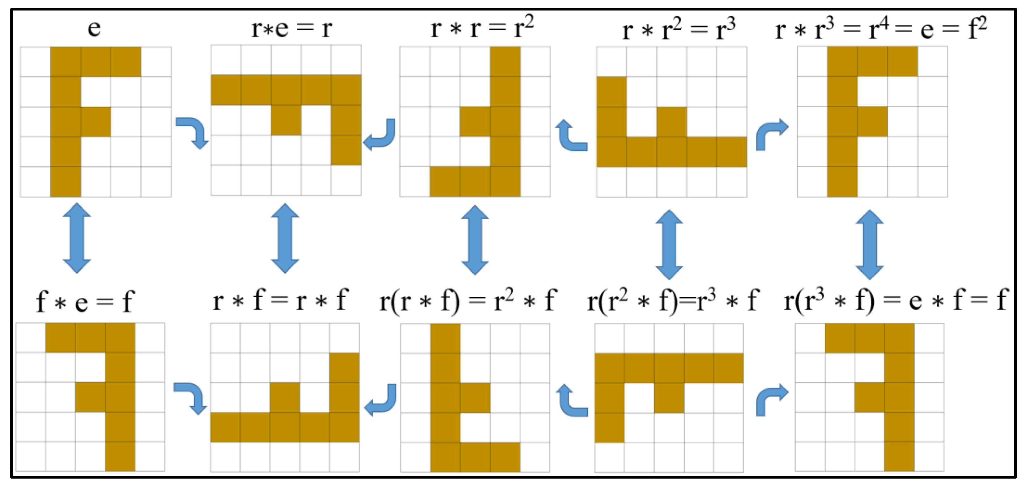
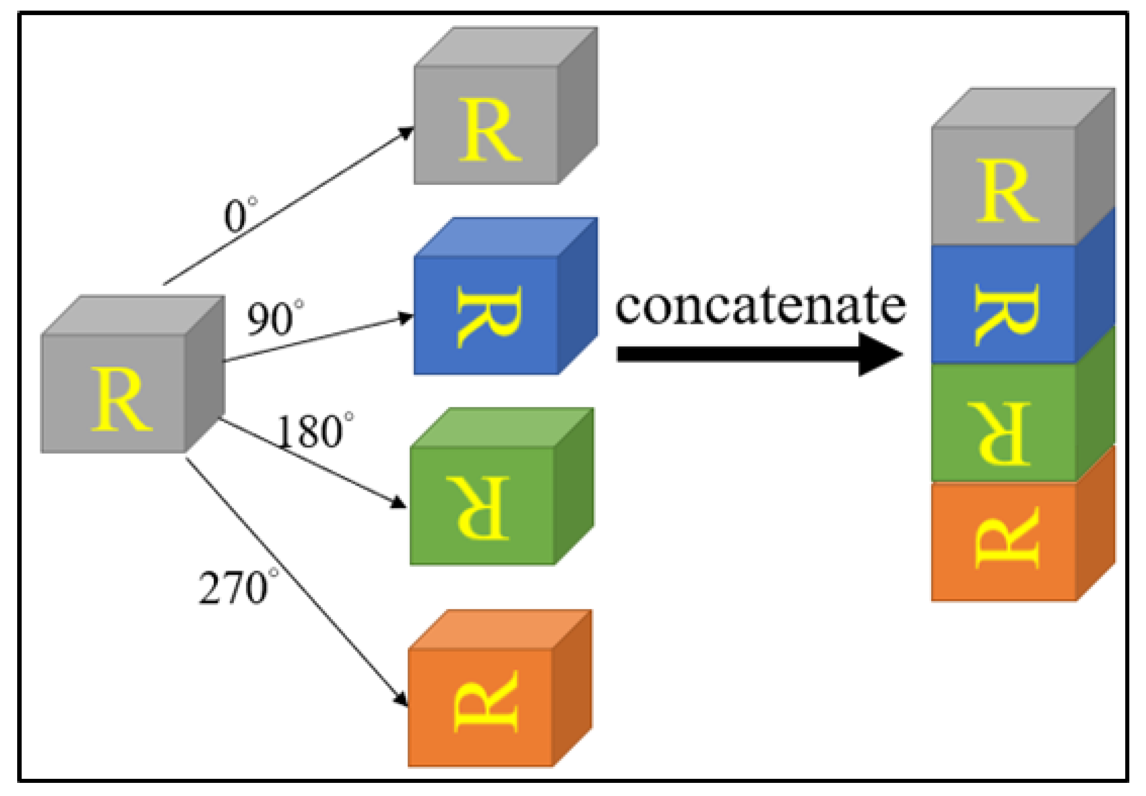
2.1. Rotation Invariance and the Dihedral Group D4 (Dih4)
2.2. Multi-Scale Learning
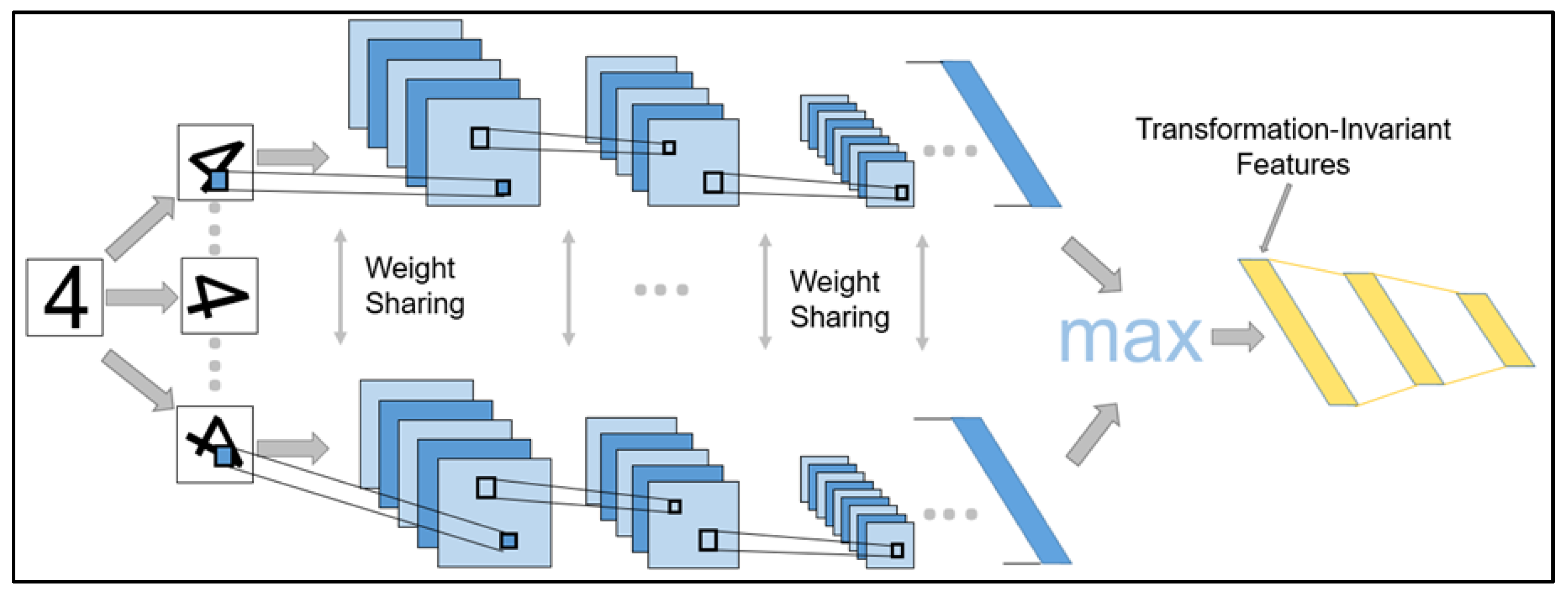
2.3. TI-Pooling CNN
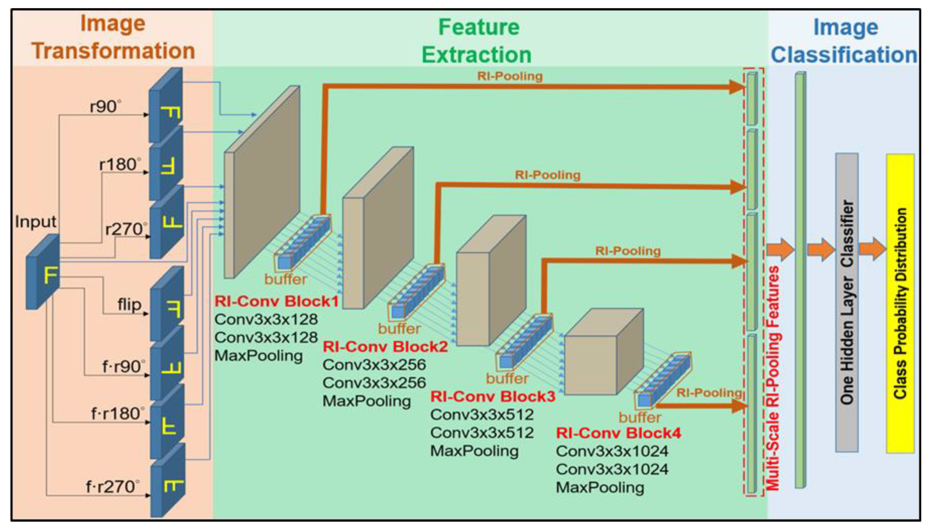
3. Methods
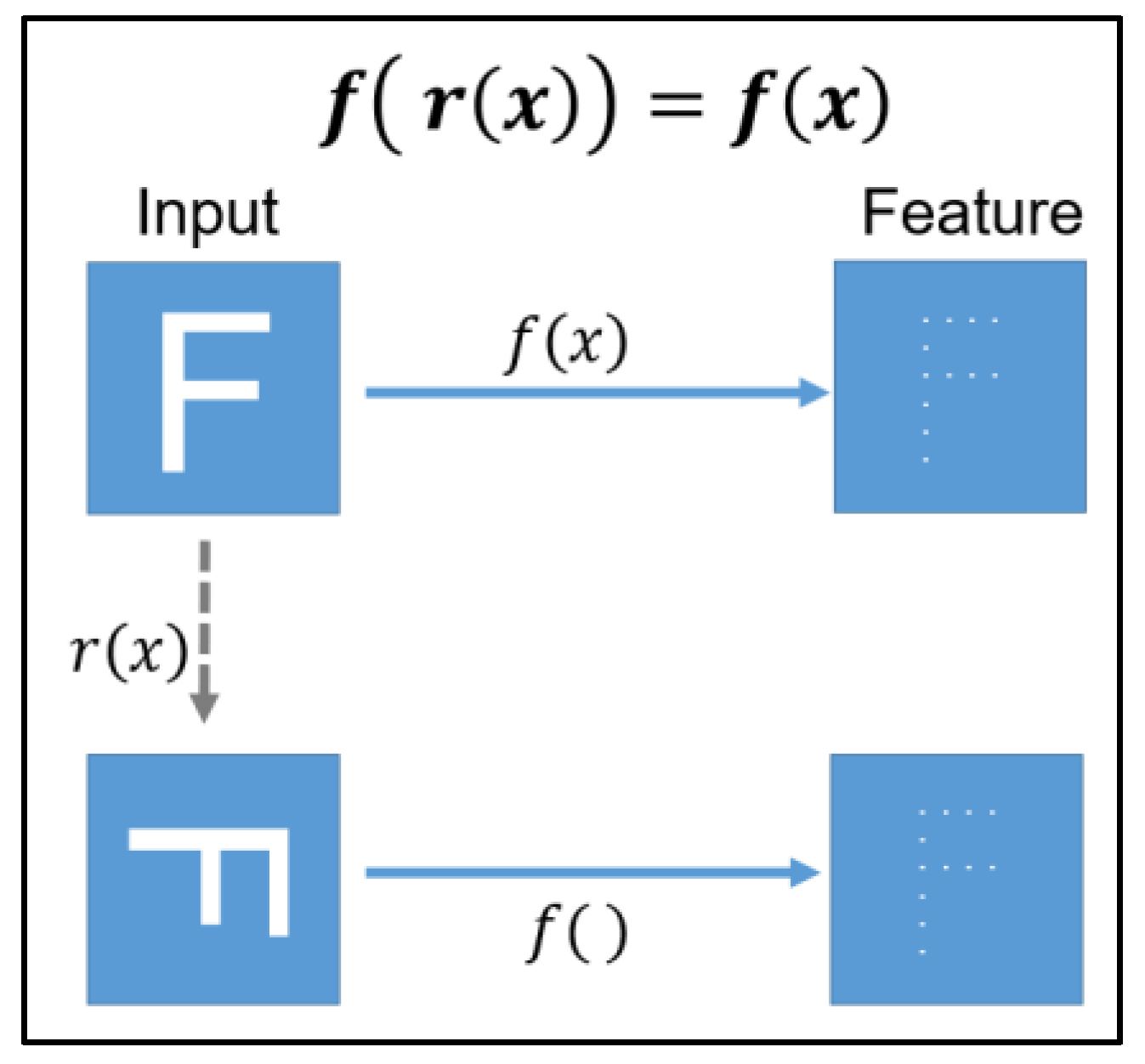
3.1. Image Transformation
3.2. Feature Extraction
3.2.1. RI-Conv Block Structure
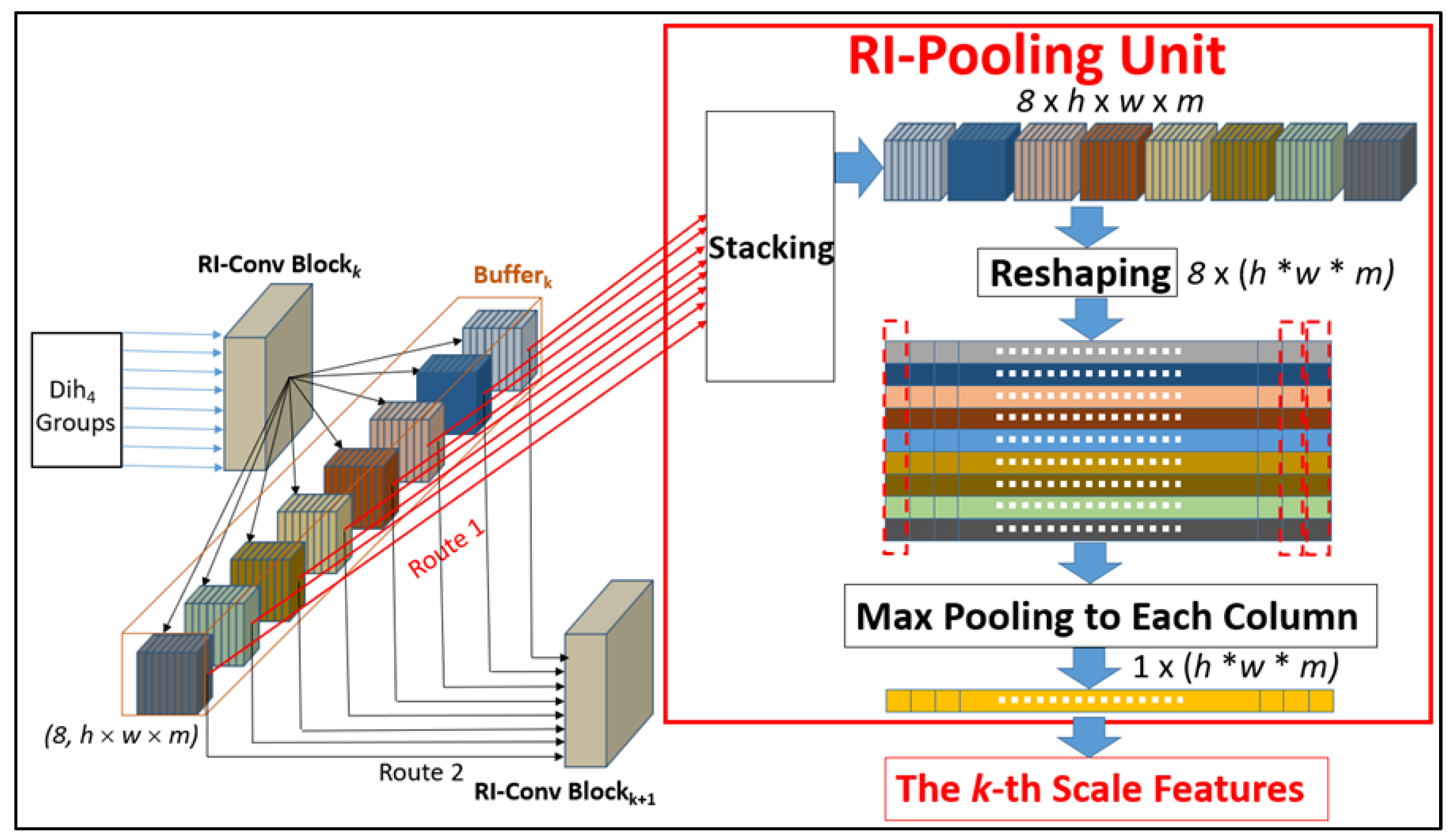
3.2.2. Buffers in the RIMS-CNN Architecture
3.2.3. Rotation-Invariant Pooling (RI-Pooling) Unit
3.3. Image Classification
3.4. Time Complexity of RIMS-CNN
4. Experimental Results and Discussion
4.1. Datasets and Preprocessing
4.2. Experimental Settings
4.3. Experimental Results
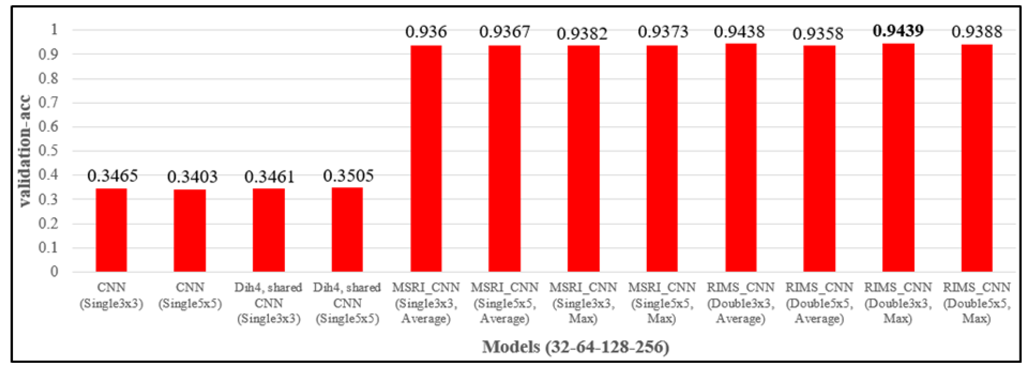
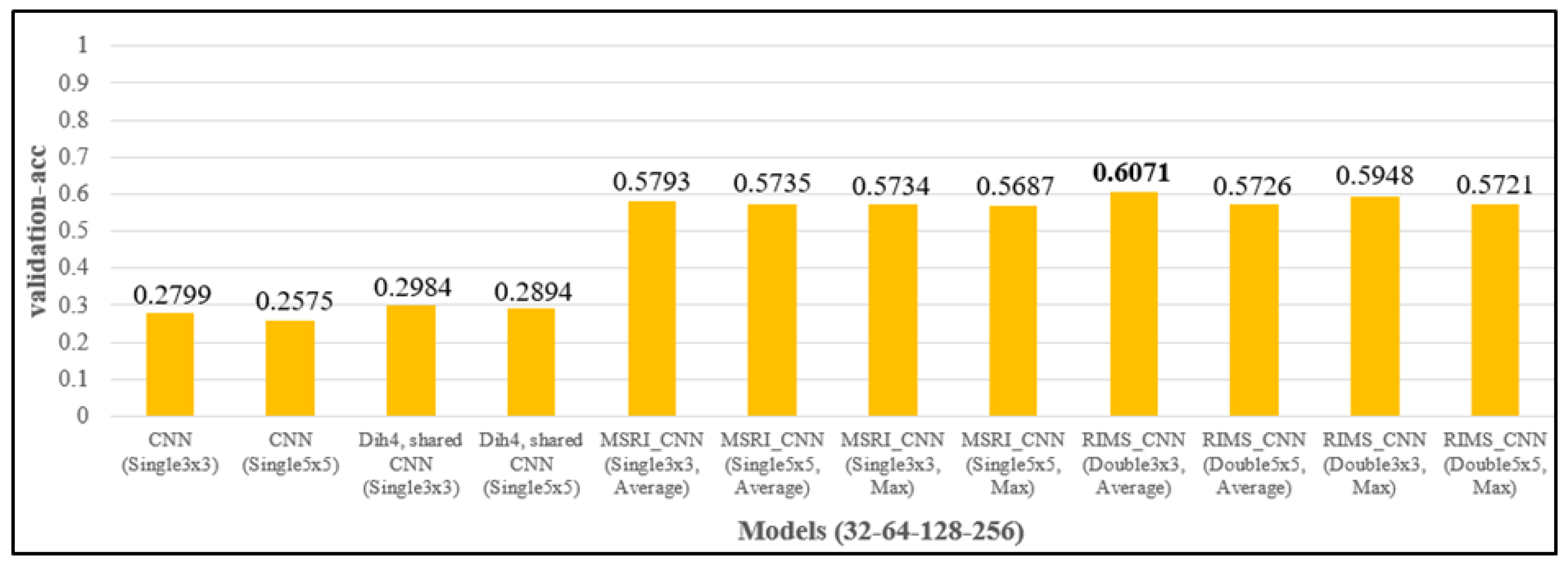
4.3.1. Different Design of the Feature Extraction Layers
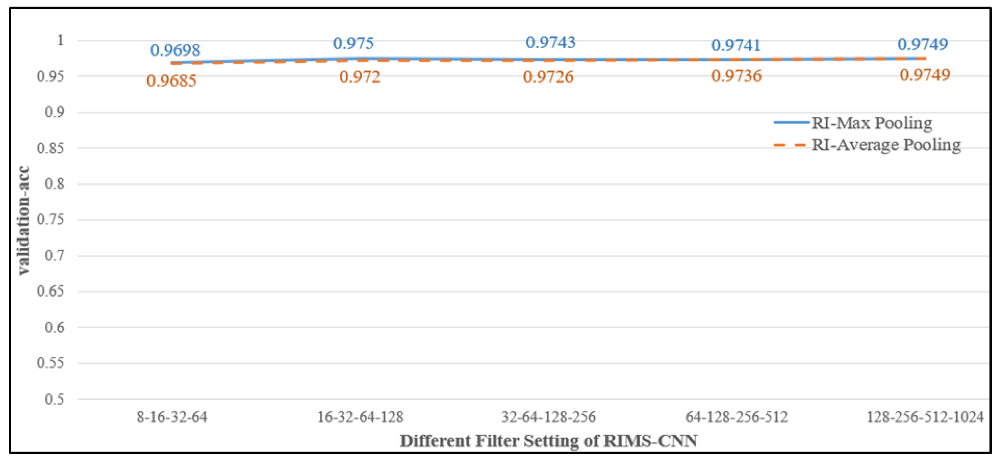
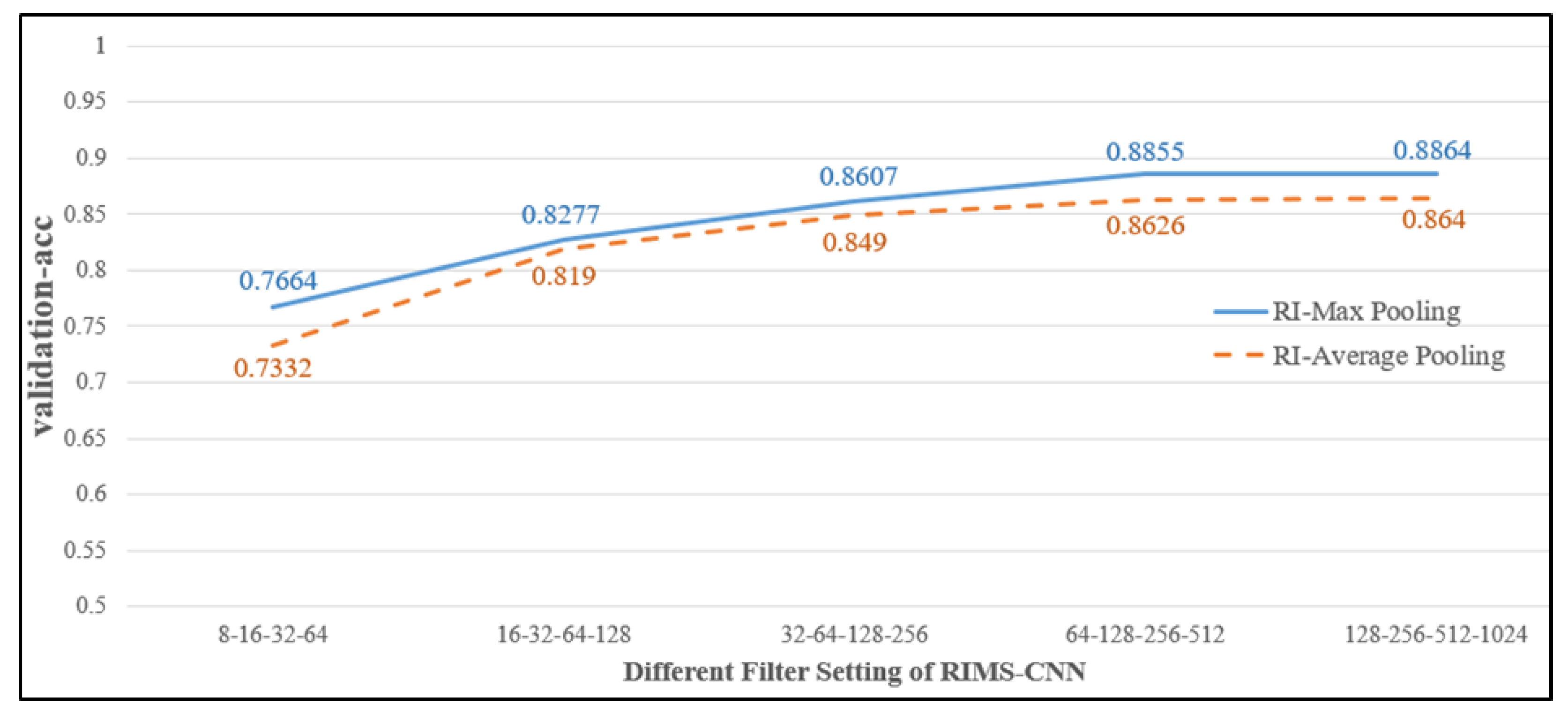
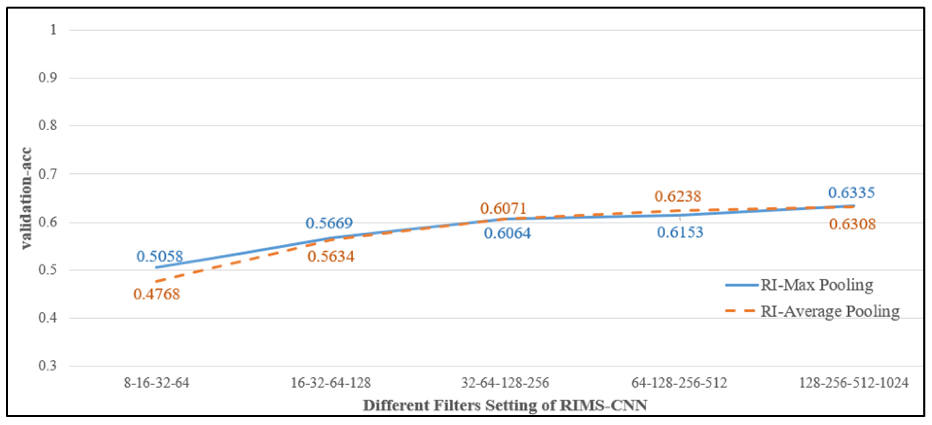
4.3.2. Comparing RI-Max Pooling with RI-Average Pooling in Different Filters of RIMS-CNN
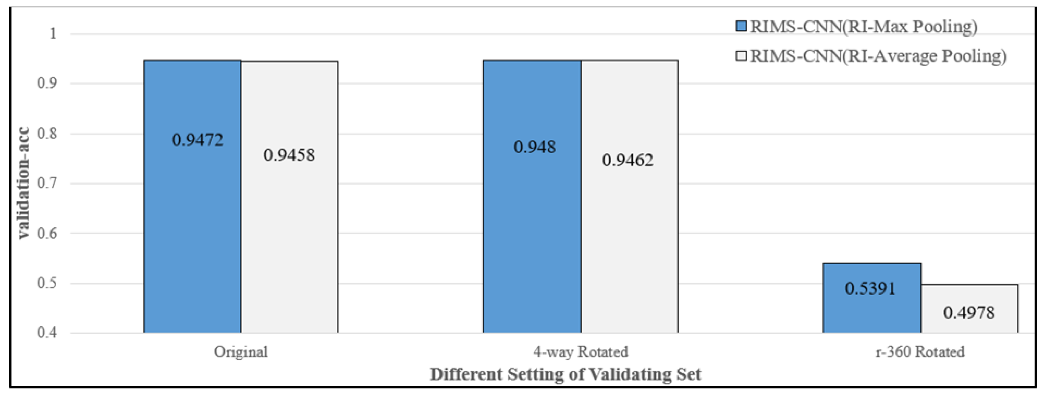
4.3.3. Comparing RI-Max Pooling with RI-Average Pooling in Different Datasets
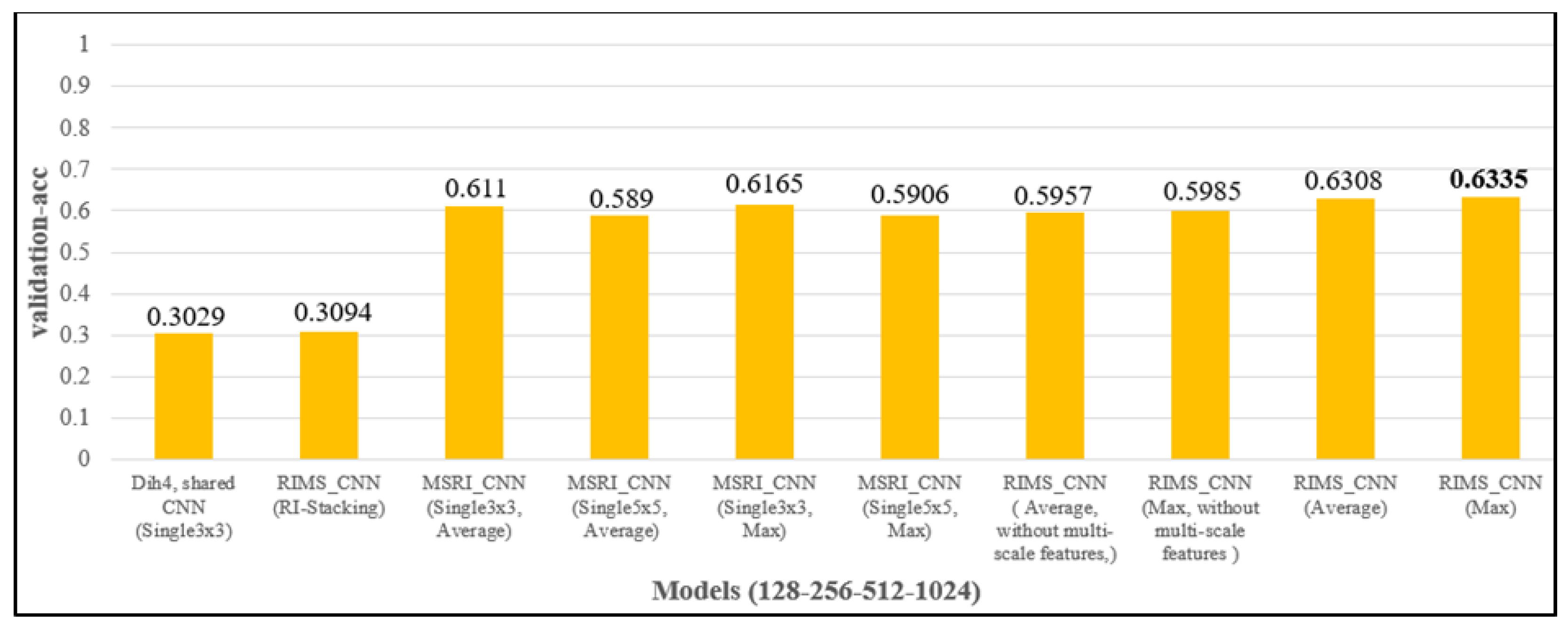
4.3.4. Evaluating Different Feature-Extracting Structures in RIMS-CNN
4.3.5. Evaluating Models on Original Training Sets and Validating Sets
4.3.6. Evaluating Models on Original Training Sets and Fixed-Angle Rotated Validating Sets
4.3.7. Evaluating Models on Fixed-Angle Rotated Training Sets and Fixed-Angle Rotated Validating Sets
4.3.8. Evaluating Models on Fixed-Angle Rotated Training Sets and Random-Angle Rotated Validating Sets
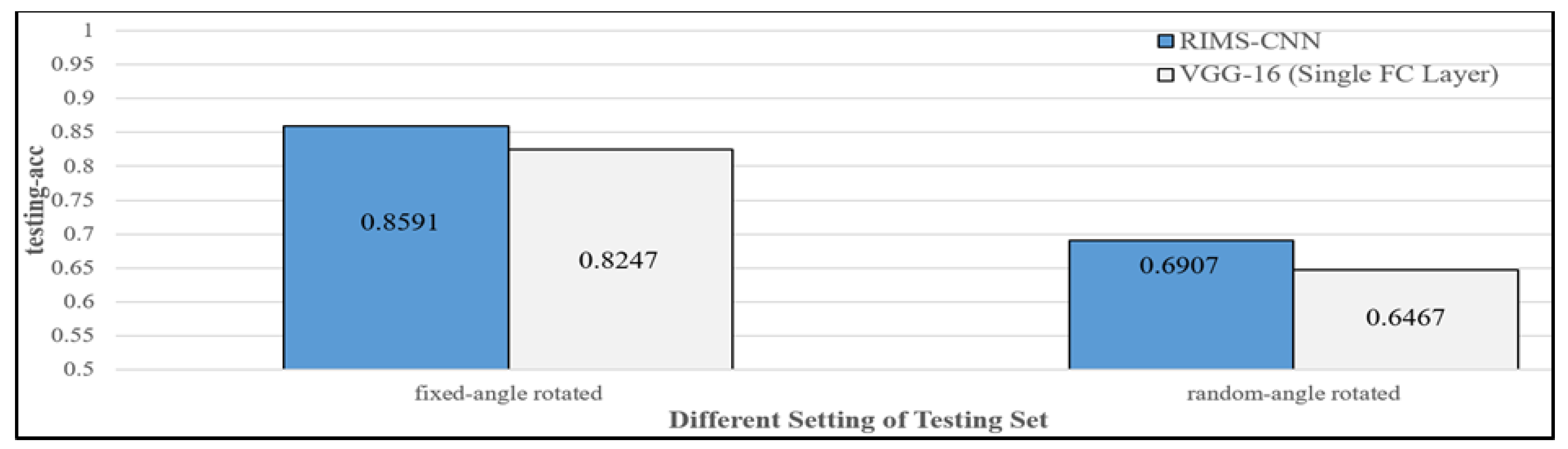
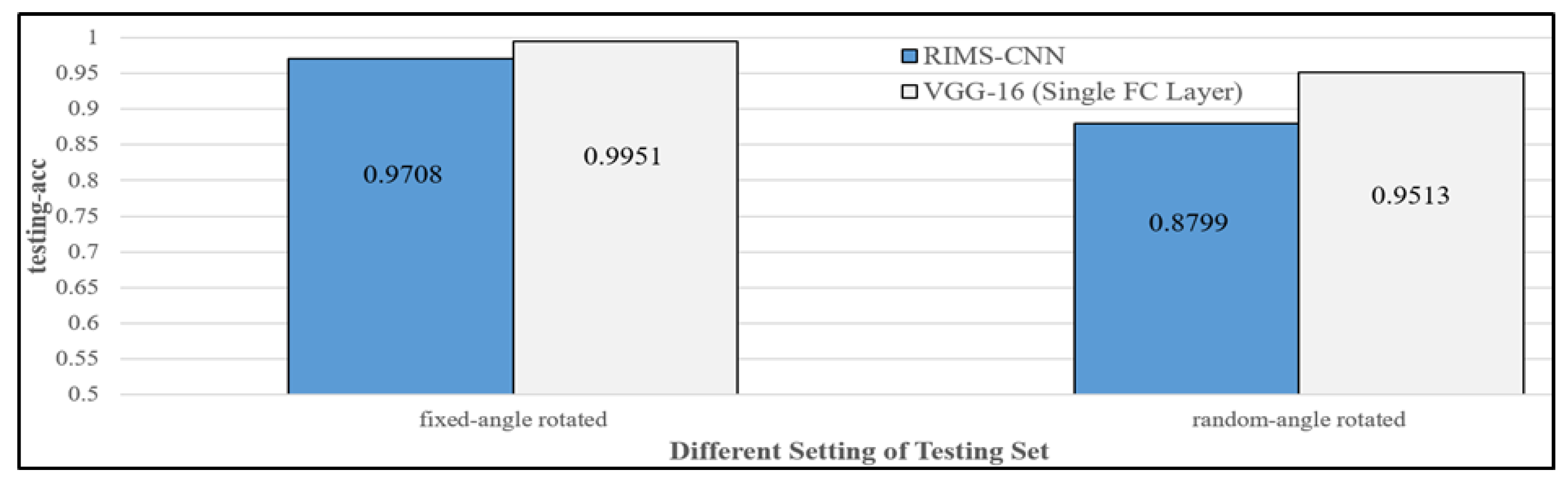
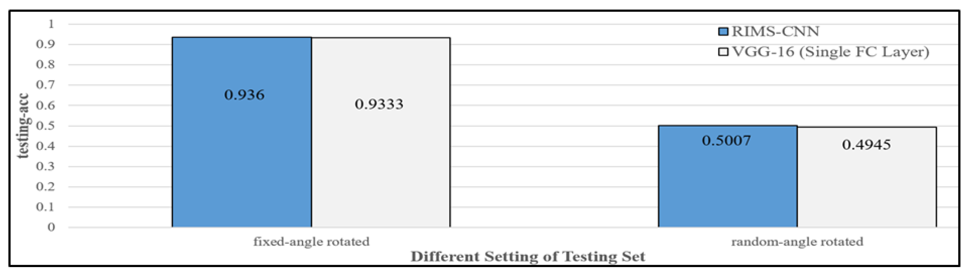
4.3.9. Evaluating RIMS-CNN and VGG-16 on Fixed-Angle Rotated Testing Sets and Random-Angle Testing Sets
4.3.10. Comparison of RIMS-CNN and Some Other Rotation-Invariant Models
5. Conclusions and Future Work
Author Contributions
Funding
Data Availability Statement
Conflicts of Interest
References
- Lecun, Y.; Bottou, L.; Bengio, Y.; Haffner, P. Gradient-based learning applied to document recognition. Proc. IEEE 1998, 86, 2278–2324. [Google Scholar] [CrossRef] [Green Version]
- Krizhevsky, A.; Sutskever, I.; Hinton, G.E. ImageNet classification with deep convolutional neural networks. In Proceedings of the Neural Information Processing Systems (NIPS), Stateline, NV, USA, 3–8 December 2012; pp. 1097–1105. [Google Scholar]
- Simonyan, K.; Zisserman, A. Very deep convolutional networks for large-scale image recognition. In Proceedings of the International Conference on Learning Representations (ICLR), San Diego, CA, USA, 7–9 May 2015. [Google Scholar]
- He, K.; Zhang, X.; Ren, S.; Sun, J. Deep residual learning for image recognition. In Proceedings of the IEEE Computer Vision and Pattern Recognition (CVPR), Las Vegas, NV, USA, 27–30 June 2016; pp. 770–778. [Google Scholar]
- He, K.; Zhang, X.; Ren, S.; Sun, J. Identity mappings in deep residual networks. In Proceedings of the European Conference on Computer Vision (ECCV), Amsterdam, The Netherlands, 8–16 October 2016; pp. 630–645. [Google Scholar]
- Szegedy, C.; Liu, W.; Jia, Y.; Sermanet, P.; Reed, S.; Anguelov, D.; Erhan, D.; Vanhoucke, V.; Rabinovich, A. Going deeper with convolutions. In Proceedings of the IEEE Computer Vision and Pattern Recognition (CVPR), Boston, MA, USA, 7–12 June 2015; pp. 1–9. [Google Scholar]
- Szegedy, C.; Vanhoucke, V.; Ioffe, S.; Shlens, J.; Wojna, Z. Rethinking the Inception architecture for computer vision. In Proceedings of the IEEE Computer Vision and Pattern Recognition (CVPR), Las Vegas, NV, USA, 27–30 June 2016; pp. 2818–2826. [Google Scholar]
- Huang, G.; Liu, Z.; Van Der Maaten, L.; Weinberger, K.Q. Densely connected convolutional networks. In Proceedings of the IEEE Computer Vision and Pattern Recognition (CVPR), Honolulu, HI, USA, 21–26 July 2017; pp. 4700–4708. [Google Scholar]
- Gens, R.; Domingos, P.M. Deep symmetry networks. In Proceedings of the Neural Information Processing Systems (NIPS), Montréal, QC, Canada, 8–11 December 2014; pp. 2537–2545. [Google Scholar]
- Lo, S.C.B.; Freedman, M.T.; Mun, S.K.; Gu, S. Transformationally identical and invariant convolutional neural networks through symmetric element operators. arXiv 2018, arXiv:1806.03636. [Google Scholar]
- Jain, A.; Sai Subrahmanyam, G.R.K.; Mishra, D. Stacked features based CNN for rotation invariant digit classification. In Proceedings of the Pattern Recognition and Machine Intelligence (PReMI), Kolkata, India, 5–8 December 2017; pp. 527–533. [Google Scholar]
- Kang, S. Rotation-invariant wafer map pattern classification with convolutional neural networks. IEEE Access 2020, 8, 170650–170658. [Google Scholar] [CrossRef]
- Laptev, D.; Savinov, N.; Buhmann, J.M.; Pollefeys, M. Ti-pooling: Transformation-invariant pooling for feature learning in convolutional neural networks. In Proceedings of the IEEE Conference on Computer Vision and Pattern Recognition (CVPR), Las Vegas, NV, USA, 27–30 June 2016; pp. 289–297. [Google Scholar]
- Dieleman, S.; Willett, K.W.; Dambre, J. Rotation-invariant convolutional neural networks for galaxy morphology prediction. Mon. Not. R. Astron. Soc. 2015, 450, 1441–1459. [Google Scholar] [CrossRef]
- Dieleman, S.; De Fauw, J.; Kavukcuoglu, K. Exploiting cyclic symmetry in convolutional neural networks. arXiv 2016, arXiv:1602.02660. [Google Scholar]
- Wu, F.; Hu, P.; Kong, D. Flip-rotate-pooling convolution and split dropout on convolution neural networks for image classification. arXiv 2015, arXiv:1507.08754. [Google Scholar]
- Marcos, D.; Volpi, M.; Tuia, D. Learning rotation invariant convolutional filters for texture classification. In Proceedings of the International Conference on Pattern Recognition (ICPR), Cancun, Mexico, 4–8 December 2016; pp. 2012–2017. [Google Scholar]
- Lo, S.B.; Freedman, M.T.; Mun, S.K.; Chan, H.-P. Geared rotationally identical and invariant convolutional neural network Systems. arXiv 2018, arXiv:1808.01280. [Google Scholar]
- Kim, J.; Jung, W.; Kim, H.; Lee, J. CyCNN: A rotation invariant CNN using polar mapping and cylindrical convolutional layers. arXiv 2020, arXiv:2007.10588. [Google Scholar]
- Woods, J.W. Multidimensional Signal, Image, and Video Processing and Coding, 2nd ed.; Academic Press: London, UK, 2011; pp. 28–30. [Google Scholar]
- Judson, T.W. Abstract Algebra: Theory and Applications; Virginia Commonwealth University Mathematics: Richmond, VA, USA, 2009; pp. 81–83. [Google Scholar]
- Liu, W.; Anguelov, D.; Erhan, D.; Szegedy, C.; Reed, S.; Fu, C.-Y.; Berg, A.C. SSD: Single shot multibox detector. In Proceedings of the European Conference on Computer Vision (ECCV), Amsterdam, The Netherlands, 8–16 October 2016; pp. 21–37. [Google Scholar]
- MNIST Handwritten Digit Database. Yann LeCun, Corinna Cortes and Chris Burges. Available online: http://yann.lecun.com/exdb/mnist/ (accessed on 17 December 2021).
- Xiao, H.; Rasul, K.; Vollgraf, R. Fashion-mnist: A novel image dataset for benchmarking machine learning algorithms. arXiv 2017, arXiv:1708.07747. [Google Scholar]
- CIFAR-10 and CIFAR-100 Datasets. Available online: https://www.cs.toronto.edu/~kriz/cifar.html (accessed on 17 December 2021).
- Kingma, D.P.; Ba, J. Adam: A method for stochastic optimization. arXiv 2014, arXiv:1412.6980. [Google Scholar]
- Prechelt, L. Early stopping-but when? In Neural Networks: Tricks of the Trade, 2nd ed.; Müller, O., Ed.; Springer: Berlin/Heidelberg, Germany, 1998; pp. 53–67. [Google Scholar]
- Zhou, Y.; Ye, Q.; Qiu, Q.; Jiao, J. Oriented response networks. In Proceedings of the IEEE Computer Vision and Pattern Recognition (CVPR), Honolulu, HI, USA, 21–26 July 2017; pp. 4961–4970. [Google Scholar]
- Follmann, P.; Bottger, T. A rotationally-invariant convolution module by feature map back-rotation. In Proceedings of the IEEE Winter Conference on Applications of Computer Vision (WACV), Lake Tahoe, NV, USA, 12–15 March 2018; pp. 784–792. [Google Scholar]
- Salas, R.R.; Dokladalova, E.; Dokladal, P. Rotation invariant CNN using scattering transform for image classification. In Proceedings of the 2019 IEEE International Conference on Image Processing (ICIP), Taipei, Taiwan, 22–25 September 2019; pp. 654–658. [Google Scholar]


| Dataset | Number of Training Set | Number of Testing Set | Image Size | Class Number |
|---|---|---|---|---|
| MNIST | 60,000 | 10,000 | 28 × 28 × 1 | 10 |
| FASHION-MNIST | 60,000 | 10,000 | 28 × 28 × 1 | 10 |
| CIFAR-10 | 60,000 | 10,000 | 32 × 32 × 3 | 10 |
| CIFAR-100 | 60,000 | 10,000 | 32 × 32 × 3 | 100 |
| Dataset | Class | Number | Dataset | Class | Number | Dataset | Class | Number |
|---|---|---|---|---|---|---|---|---|
| MNIST | 1 | 980 | FASHION-MNIST and CIFAR-10 | 1 | 1000 | CIFAR-100 | 1 | 100 |
| 2 | 1135 | 2 | 1000 | 2 | 100 | |||
| 3 | 1032 | 3 | 1000 | 3 | 100 | |||
| 4 | 1010 | 4 | 1000 | … | … | |||
| 5 | 982 | 5 | 1000 | |||||
| 6 | 892 | 6 | 1000 | |||||
| 7 | 958 | 7 | 1000 | 97 | 100 | |||
| 8 | 1028 | 8 | 1000 | 98 | 100 | |||
| 9 | 974 | 9 | 1000 | 99 | 100 | |||
| 10 | 1009 | 10 | 1000 | 100 | 100 |
| Models | Accuracy of the Original Validating Sets | |||
|---|---|---|---|---|
| MNIST | FASHION-MNIST | CIFAR-10 | CIFAR-100 | |
| RIMS-CNN (Single FC Layer) | 0.9756 | 0.9472 | 0.88 | 0.6312 |
| DenseNet121 (Single FC Layer) | 0.9962 | 0.9158 | 0.7635 | 0.4461 |
| MobileNetV2 (Single FC Layer) | 0.9952 | 0.9176 | 0.6887 | 0.3149 |
| ResNet50V2 (Single FC Layer) | 0.9962 | 0.9206 | 0.7467 | 0.4386 |
| VGG-16 (Single FC Layer) | 0.9967 | 0.938 | 0.8611 | 0.5267 |
| InceptionV3 (Single FC Layer) | 0.9962 | 0.9237 | 0.7742 | 0.405 |
| Models | Accuracy of the Fixed-Angle Rotated Validating Sets | |||
|---|---|---|---|---|
| MNIST | FASHION-MNIST | CIFAR-10 | CIFAR-100 | |
| RIMS-CNN (Single FC Layer) | 0.9756 | 0.9472 | 0.88 | 0.6312 |
| TI-Pooling (Single FC Layer) | 0.9799 | 0.9229 | 0.7524 | 0.5042 |
| DenseNet121 (Single FC Layer) | 0.4475 | 0.3267 | 0.4373 | 0.2358 |
| MobileNetV2 (Single FC Layer) | 0.4329 | 0.3469 | 0.3945 | 0.1768 |
| ResNet50V2 (Single FC Layer) | 0.4166 | 0.3306 | 0.4187 | 0.2218 |
| VGG-16 (Single FC Layer) | 0.4438 | 0.3402 | 0.4645 | 0.2645 |
| InceptionV3 (Single FC Layer) | 0.3465 | 0.345 | 0.3057 | 0.1172 |
| Models | Accuracy of the Fixed-Angle Rotated Training Sets | |||
|---|---|---|---|---|
| MNIST | FASHION-MNIST | CIFAR-10 | CIFAR-100 | |
| RIMS-CNN (Single FC Layer) | 0.9756 | 0.9472 | 0.88 | 0.6312 |
| TI-Pooling (Single FC Layer) | 0.9799 | 0.9229 | 0.7524 | 0.5042 |
| DenseNet121 (Single FC Layer) | 0.9954 | 0.9188 | 0.7692 | 0.4564 |
| MobileNetV2 (Single FC Layer) | 0.9936 | 0.9196 | 0.6903 | 0.3563 |
| ResNet50V2 (Single FC Layer) | 0.9953 | 0.9223 | 0.75 | 0.4128 |
| VGG-16 (Single FC Layer) | 0.9956 | 0.9398 | 0.8442 | 0.5375 |
| InceptionV3 (Single FC Layer) | 0.9951 | 0.9232 | 0.2046 | 0.0325 |
| Models | Accuracy of the Random-Angle Rotated Validating Sets | |||
|---|---|---|---|---|
| MNIST | FASHION-MNIST | CIFAR-10 | CIFAR-100 | |
| RIMS-CNN (Single FC Layer) | 0.891 | 0.5391 | 0.7083 | 0.4846 |
| TI-Pooling (Single FC Layer) | 0.8869 | 0.5338 | 0.6343 | 0.3898 |
| DenseNet121 (Single FC Layer) | 0.9499 | 0.4913 | 0.6167 | 0.3626 |
| MobileNetV2 (Single FC Layer) | 0.9293 | 0.4727 | 0.5685 | 0.2766 |
| ResNet50V2 (Single FC Layer) | 0.9461 | 0.4831 | 0.5844 | 0.3314 |
| VGG-16 (Single FC Layer) | 0.9481 | 0.494 | 0.6723 | 0.4167 |
| InceptionV3 (Single FC Layer) | 0.9217 | 0.5435 | 0.5363 | 0.2168 |
| Model | Accuracy | ||
|---|---|---|---|
| MNIST | CIFAR-10 | CIFAR-100 | |
| RIMS-CNN (Single FC Layer) (ours) | 0.891 | 0.7083 | 0.4846 |
| TI-Pooling (Single FC Layer) | 0.8869 | 0.6343 | 0.3898 |
| ORN-8 (ORPooling) [28] | 0.8333 | - | - |
| ORN-8 (ORAlign) [28] | 0.8379 | - | - |
| ORN [28] | - | 0.4069 | 0.2164 |
| RotInv Conv. (RP_RF_1) [29] | 0.8015 | - | - |
| RotInv Conv. (RP_RF_1_32) [29] | 0.8780 | - | - |
| RotInv Conv. (RP 1234) [29] | - | 0.4412 | 0.2294 |
| Covariant CNN [30] | 0.8279 | - | - |
Publisher’s Note: MDPI stays neutral with regard to jurisdictional claims in published maps and institutional affiliations. |
© 2022 by the authors. Licensee MDPI, Basel, Switzerland. This article is an open access article distributed under the terms and conditions of the Creative Commons Attribution (CC BY) license (https://creativecommons.org/licenses/by/4.0/).
Share and Cite
Hong, T.-P.; Hu, M.-J.; Yin, T.-K.; Wang, S.-L. A Multi-Scale Convolutional Neural Network for Rotation-Invariant Recognition. Electronics 2022, 11, 661. https://doi.org/10.3390/electronics11040661
Hong T-P, Hu M-J, Yin T-K, Wang S-L. A Multi-Scale Convolutional Neural Network for Rotation-Invariant Recognition. Electronics. 2022; 11(4):661. https://doi.org/10.3390/electronics11040661
Chicago/Turabian StyleHong, Tzung-Pei, Ming-Jhe Hu, Tang-Kai Yin, and Shyue-Liang Wang. 2022. "A Multi-Scale Convolutional Neural Network for Rotation-Invariant Recognition" Electronics 11, no. 4: 661. https://doi.org/10.3390/electronics11040661
APA StyleHong, T.-P., Hu, M.-J., Yin, T.-K., & Wang, S.-L. (2022). A Multi-Scale Convolutional Neural Network for Rotation-Invariant Recognition. Electronics, 11(4), 661. https://doi.org/10.3390/electronics11040661