Change Detection in Remote Sensing Image Data Comparing Algebraic and Machine Learning Methods

Abstract

Remote sensing technology has penetrated all the natural resource segments as it provides precise information in an image mode. Remote sensing satellites are currently the fastest-growing source of geographic area information. With the continuous change in the earth’s surface and the wide application of remote sensing, change detection is very useful for monitoring environmental and human needs. So, it is necessary to develop automatic change detection techniques to improve the quality and reduce the time required by manual image analysis. This work focuses on the improvement of the classification accuracy of the machine learning techniques by reviewing the training samples and comparing the post-classification comparison with the image differencing in the algebraic technique. Landsat data are medium spatial resolution data; that is why pixel-wise computation has been applied. Two change detection techniques have been studied by applying a decision tree algorithm using a separability matrix and image differencing. The first change detection, e.g., the separability matrix, is a post-classification comparison in which individual images are classified by a decision tree algorithm. The second change detection is, e.g., the image differencing change detection technique in which changed and unchanged pixels are determined by applying the corner method to calculate the threshold on the changing image. The performance of the machine learning algorithm has been validated by 10-fold cross-validation. The experimental results show that the change detection using the post-classification method produced better results when compared to the image differencing of the algebraic change detection technique.

1. Introduction

Change detection is the process of finding and evaluating access points in multi-spectra images that have undergone spatial or spectral changes. Change detection is often defined as the comparison of two co-registered views of the same geographic area captured at successive periods. The ability to recognize the possible label change on the ground is enabled by the availability of shots of the same geographic area taken by sensors at different periods. Change detection is the process of identifying a group of pixels in a prior dataset that has changed significantly. Remote sensing plays a significant role in a variety of application areas, including land cover classification, deforestation, disaster monitoring, glacier management, urban expansion monitoring, and environmental study change detection. Understanding the linkages and interactions between human and natural phenomena and promoting improved decision making requires timely and precise change detection of the earth’s surface.

With the utility of change detection in many remote sensing applications, manual change identification utilizing sequential pictures is a difficult process [1]. Due to a wide range of applications in various fields, detecting and distinguishing changes in photographs of the same scene acquired at different times has piqued the interest of scholars for many years. Remotely sensed data have been an important source of information for many change detection applications in recent decades [2] due to the advantages of recurring data gathering, the synoptic view of multitemporal images, and the digital format appropriate for computer processing. It is critical to create effective and automatic change detection systems to fully harness the massive amounts of data collected by today’s remote sensing satellites. This is a hot topic right now, and new strategies are needed to make the most of the growing and diversified remote sensing data.

The motivation of this work is to study the impact of different image capturing techniques, remote sensors, and digital image processing techniques. This work presents a basic introduction of remote sensors and image capture techniques. The study in this work focuses on the comparison of machine learning and algebraic techniques. As ground truthing is outside the scope of this study, the objective of the proposed study is to review the training of classifiers to improve the classifier accuracy of the machine learning techniques and compare them with the algebraic techniques for change detection in remote sensing images. The main objectives of the work are:

• To apply the decision tree induction algorithm, using the separability matrix on both the images for a post-classification comparison of the change detection.
• To apply the algebraic technique of image differencing, using the corner method to discover the changed and unchanged areas.

This work’s organization is as follows: in Section 2, the basic concepts of remote sensing images and change detection are described. This section also includes the different ways of data acquisition and the existing change detection techniques. Algebra-based, transformation-based, classification-based, advanced model, GIS, visual analysis, and other change detection techniques are presented here. In Section 3, some related work is presented. Section 4 contains the proposed approaches, including two algorithms: a decision tree algorithm, using the class separability matrix, and image differencing, using the corner method, to discover the presented change detection. Section 4 contains the proposed approaches: a decision tree algorithm, using the class separability matrix, and image differencing, using the corner method, to discover the change detection. Section 5 comprises the detailed description of the implementation, experiments, results, and analysis of the change detection techniques with machine learning and algebraic techniques. The results of the decision tree algorithm, using the class separability matrix, and image differencing, using the corner method, are shown in false-color images.

2. Basics of Remote Sensing and Change Detection Process

Remote sensing is the process of recording, measuring, and analyzing images and digital representations of energy patterns derived from non-contact sensor devices in order to gather trustworthy information about physical things and the environment [3]. Remote sensing technology has pierced into every segment of the natural resources as it provides clear information in an image mode. Every object in the universe reflects, radiates, or scatters electromagnetic radiation. Remote sensing is a technique or tool similar to mathematics. Sensors are used to measure the amount of radiation radiated by an object or geographic area from a distance, and with the help of statistical- and mathematical-based algorithms, some valuable information is extracted. An interaction model depicting the relationship of remote sensing with the social, physical, and biological sciences and with mathematics and logic is shown in Figure 1. The general remote sensing process used by the scientists for extracting information from remotely sensed data is carried out in four steps, as shown in Figure 2. In this subsection, different ways of remote sensing data acquisition and change detection processes have been covered.

2.1. Remote Sensing Data Acquisition Methods

Remotely sensed data collection is the most important and expensive job in the remote sensing process. It is essential to have remotely sensed images in a digital format to apply digital image processing. There are two fundamental ways to acquire the digital image:

• Capture the image with a remote sensing device in an analogue format, then convert it to digital format.
• Take a digital image of the remotely sensed image, such as one obtained by the Landsat 7 Thematic Mapper sensor system.

The ability of a system to render information at the smallest discretely separable quantity in terms of space (spatial), EMR wavelength band (spectral), time (temporal), and/or radiation quantity is characterized as resolution (radiometric). Some of the major parameters that determine the nature of the collected remote sensing data are discussed in the subsections below.

2.1.1. Spectral Information and Resolution

The dimension (size) and the number of specific bands or channels in the electromagnetic spectrum to which a remote sensing sensor is sensitive are spectral resolutions. The data are collected in many bands of the electromagnetic spectrum by a multispectral remote sensing sensor. The data are collected in hundreds of spectral bands by a hyperspectral remote sensing device. Energy is recorded in hundreds of bands by an ultra-spectral remote sensing system. The bands are usually chosen to maximize the contrast between the object and the background. As a result, appropriate band selection may increase the likelihood of retrieving the needed information from the remote sensor data. The greater the narrowness of the band, the greater the spectral resolution.

2.1.2. Spatial Information and Resolution

The lowest angular or linear gap between two objects that a remote sensing system can resolve is called the spatial resolution. Using the spatial information in the image, the amount of spectral autocorrelation may be estimated. A pixel is a small spot on the earth’s surface that a sensor can observe as being distinct from its surroundings. It is a detector element or a slit whenever projected onto the ground. In other words, the ground segment sensed at any one time is the scanner’s spatial resolution. It has sometimes been referred to as the ground resolution element (GRE). The spatial resolution at which data is obtained affects the ability to distinguish diverse features and measure their extent. According to the usual rule, the spatial resolution should be less than half the size of the smallest object of interest.

2.1.3. Temporal Information and Resolution

The temporal resolution refers to how often a sensor records an image of a specific area. For many applications, a high temporal resolution is critical. Temporal resolution refers to the satellite’s capacity to extract the same area from the same viewing angle at different times. A sensor’s temporal resolution is determined by several elements, including the satellite/sensor capabilities, swath overlap, and latitude.

2.1.4. Radiometric Information and Resolution

The sensitivity of detectors to minor variations in electromagnetic energy is known as radiometric resolution. High radiometric resolution improves the likelihood of more accurate remote sensing of phenomena. A sensor measurement allows it to distinguish the tiniest variation in spectral reflectance/remittance between different targets. The number of quantization levels and the saturation radiance determine the radiometric resolution. The more tiers there are, the more detailed the information that becomes digitalized.

2.1.5. Polarization Information

The polarization characteristics of electromagnetic radiation collected by remote sensing systems can be utilized to investigate the earth’s resources. In general, the stronger the polarization, the smoother the object’s surface.

2.1.6. Angular Information

The angle of incidence has traditionally been related to the incoming energy that illuminates the landscape and the angle of exitance from the terrain to the sensor system. The bidirectional nature of the remote sensing data collection influences the spectrum and polarization of the sensor light collected by the remote sensing system [3,4].

2.2. Remote Sensing Data Acquisition

The two important methods of remote sensing data acquisition are aerial photography and satellite image data collection. Aerial photographs are the snapshots of the earth taken by calibrated cameras at a particular instant of time in an analog format. Through the process of digitization, this analog format is converted into a digital format. Aerial photography can be taken from space, from high- or low-altitude airplanes, or from platforms close to the ground. Each aerial shot has vital information for the user in the margin.

• Vertical Photographs: The photographic device, i.e., the camera, is pinned as straight down as possible when taking a vertical shot. The allowed tolerance from the plumb (perpendicular) line to the camera axis is normally +3 degrees. The lens axis is nearly perpendicular to the earth’s surface, covers a limited area on a single vertical shot, and closely resembles a square or a rectangle [4].
• High oblique: The camera is tilted roughly 60 degrees from the vertical when taking a high oblique shot. It is mostly employed in the creation of aeronautical charts and has a minor military application. The ground area covered is trapezoid in high oblique images; the horizon is always visible in high oblique photographs.
• Low Oblique: This picture is taken with the camera at a 30-degree angle to the vertical. It has been used to research an area before an attack, as a replacement for a map, or as a supplement to a map. The ground area covered is a trapezoid in a low oblique area and coverage is quite limited [5].
• Trimetrogon: It is a composite of three photos shot simultaneously, one vertical and two high obliques, in a direction perpendicular to the flight path. The oblique images, taken at a 60-degree angle from the vertical, side lap the vertical photography, resulting in composites that run from horizon to horizon.

2.3. Remote Sensing Sensors

Remote sensing is performed with the help of an instrument usually referred to as a sensor. Sensors are devices designed to measure photons. A sensor is a device that collects energy (EMR or otherwise), turns it into a signal, and displays it in a manner that can be used to obtain information about the subject being investigated. A telescoping system gathers and directs radiation onto a mirror or a lens at the front end of a sensor. The mirror rapidly shakes or oscillates back and forth over a limited angular range. The scene is imaged on one swing, say forward, and the opposing or reverse swing is not scanned in this arrangement; active scanning can occur on both swings. Depending on the energy source, these can be active or passive.

Passive sensor: Passive sensors are remote sensing technologies that measure the naturally available energy.

Active Sensors: Active sensors are remote sensing devices in which energy created within the sensor’s system is beamed outward, and the return is monitored. Active remote sensing uses two types of sensors:

Across-track or whiskbroom sensor: The across-track or whiskbroom sensor normally uses a rotating or oscillating mirror, scanning the scene along with a long narrow band. It linearly scans the ground. Each line is subdivided into a series of distinct spatial elements, representing a square, rectangular, or circular space on the imaged scene surface. As a result, there is an array of contiguous cells along any line that emits radiation. Along the line, the cells are detected one by one. Each cell in the sensor has a pixel that is connected to a microelectronic detector. Each pixel has a single value of radiation. The aerial cover of the pixel is determined by IFOV (Instantaneous Field of View), which corresponds to the ground cell area of the sensor system.

Along-track or pushbroom sensor: No mirror on the along-track or pushbroom sensor looks off at different angles. Instead, there is a line of small, sensitive detectors placed one on top of the other, each with a tiny dimension on its plate surface; there are maybe thousands. A charge-coupled device is used in each detector (CCD). In this mode, the individual detectors in the line array correspond to the pixels that eventually make up the image. In a very short time, the signal is deleted from each detector in the array. The detectors are reset to zero, and they are then exposed to new radiation from the sensor’s forward motion reaching the next line on the ground. Pushbroom scanning is another name for this form of scanning.

The sensors used for remote sensing can be broadly classified as:

A. 

Optical Sensors: Scanner systems that operate outside of the visible and near-infrared ranges of the electromagnetic spectrum and in the thermal and microwave regions are all non-photographic systems. Data is gathered by a sensor system in the satellite and relayed to the ground station, where it is received and recorded. The following are some of the non-photographic data collecting systems for resource surveys that are sensitive in the visible and near-IR regions: the Thematic Mapper (TM) and the High resolution visible (HRV) Imager used in the SPOT satellite. Different types of sensors are shown in Figure 3a–f.

B. 

Microwave Remote Sensing: Microwave data can be obtained by both active and passive systems [6]. The region of the spectrum ranging between 1 mm and 1 m is designated as a microwave band. Longer wavelength microwaves can penetrate through cloud cover, haze, dust, etc. The penetration capability of microwaves helps in the detection of features under almost all weather and environmental conditions. Microwave remote sensing has the following advantages over remote sensing in the other regions of EMR. It is:

1

Time independent.

2

Weather independent.

3

Sensitive to moisture in soil, vegetation, and snow.

4

Able to penetrate soil and vegetation cover.

Microwave remote sensing is divided into two types. Thermal remote sensing is analogous to passive microwave sensing. Within its area of vision, passive microwave sensors detect naturally released microwave energy. It reacts to extremely low levels of microwave energy emitted/reflected by landscape features from ambient sources. Such sensors are used in meteorology, hydrology, and oceanography.

Microwave sensors that are active emit their microwave radiation to illuminate the target. RADAR (Radar Detection and Active Ranging) is an active microwave remote sensing system. The various systems used to describe imaging radar are Synthetic Aperture Radar (SAR), Real Aperture Radar (RAR), and the Active Microwave Imager (AMI).

2.4. Satellite Image Data Collection

Satellites are moving around the earth with the gravitational force of a central mass. The path followed by the satellite is called the orbit. These orbits are matched to the capability and objective of the sensor(s) they carry. The satellite system can provide a synoptic view and systematic and repetitive coverage. It provides multispectral information in digital format. Truly speaking, the classification of satellites is itself a misnomer. However, the concepts of the divisions are broadly [8]:

1

Remote sensing satellites (for earth observation)

2

Meteorological satellites

3

Communication satellites

Nothing is stopping the satellites from playing dual or even, for that matter, multiple roles. Take, for example, the INSAT series communication satellites. These play a dual role; they are primarily communication satellites, but they also take weather pictures. Is this not remote sensing too? Communication satellites come under two categories; they are either polar and inclined or highly elliptical and geosynchronous.

At altitudes of up to 3600 km, geosynchronous satellites are launched. Satellites in these orbits move in the same direction as the earth’s rotation, and their velocities are adjusted to keep them over a specific location on the planet’s surface. A geostationary satellite is one that “hovers” in the equatorial plane (i.e., the orbital inclination I = zero). These satellites are valuable for studies in meteorology and oceanography. Sun-synchronous satellites orbit at a significantly lower altitude than geosynchronous satellites (approximately 900 km). The orbit is at about a 90-degree inclination to the equator, and the satellites cross the equator at the same solar time each day. LANDSAT, IRS, and SPOT are some of the satellites.

Digital Image Data Format: You can order digital remote sensor data in a variety of formats. The following are the most popular formats:

BIP (Band Interleaved by Pixels): The BIP format sequentially stores the brightness value in the k bands associated with each pixel. The end of the dataset is marked with an end-of-file (EOF) marker.

BIL (Band Interleaved by Line): The BIL format sequentially records the brightness values in the k bands associated with each line. The end of the dataset is marked with an end-of-file (EOF) marker.

Band Sequential (BSQ): The BSQ format saves each band’s pixel values in a separate and distinct file. Each band has its beginning header record and an EOF marker.

2.5. Change Detection Process

The earth’s atmosphere, water, and land are astonishingly complex. This does not allow the recording of images by remote sensing devices with limitations in, for example, spatial, spectral, temporal, and radiometric resolution. The following conditions must be satisfied before implementing a change detection application.

2.5.1. Digital Image Pre-Processing

Digital image processing is the process of altering and interpreting digital photographs using a computer. Image rectification and restoration is the initial processing of raw picture data to correct geometric errors, radiometrically calibrate the data, and eliminate noise. Preprocessing activities are commonly used to describe the nature of image restoration processes because they usually come before further editing and analysis of the image data to obtain specific information. The character of such methods is influenced by the type of digital image acquisition (digital camera, across-track scanner, along-track scanner), platform (satellite vs. airborne), and total field of view. Geometric correction, radiometric correction, and noise removal are the generic terms we use to describe these activities.

2.5.2. Geometric Correction

Geometric aberrations are so common in raw digital images that they cannot be utilized as maps. These distortions can be caused by a variety of causes, including sensor platform altitude and velocity, panorama earth curvature, distortion, atmospheric refraction, nonlinearities in the IFOV sweep, and relief displacement. The goal of geometric correction is to compensate for these factors’ distortions so that the corrected image has the same geometric integrity as a map.

The geometric rectification operation is usually carried out in two steps. The systematic or predictable distortions are considered first. The second category includes distortions that are fundamentally random or unexpected.

2.5.3. Radiometric Correction

The type of radiometric correction employed to any digital image dataset varies greatly among sensors, just as it does with geometric correction. Changes in atmosphere conditions, scene illumination, and instrument response characteristics influence the radiance recorded by any given system over a given object, all other things being equal. Differences in viewing geometry, for example, are more noticeable in aerial data collection than in satellite data collection. Mosaics of images gathered over time or investigations of variations in the reflectance of ground features at different times or locations are frequently desired in satellite sensing in the visible and near-infrared range. A sun elevation adjustment and an earth–sun distance correction are necessary for such instances.

2.5.4. Noise Removal

A limitation in the sensing, signal digitization, or data-recording process causes picture noise, which is an unwanted blip in the visual data. Periodic detector drift or malfunction, electronic interference between sensor components, and occasional “hiccups” in the data transmission and recording sequence are all examples of noise sources. Noise can weaken or entirely obscure the true radiometric information content of a digital image. As a result, noise removal is typically performed before any further augmentation or classification of the image data.

2.6. Change Detection Techniques

The purpose of change detection is to compare the spatial representation of two points in time while controlling all the variations produced by differences in variables that are not of interest and assessing the changes induced by differences in the variables that are [3]. Many change detection techniques have been developed, and their use depends on the application. As part of this study, the methodology of the following multispectral change detection techniques is described/categorized into seven categories: Algebra, Transformation, Classification, Advanced Model, GIS, Visual Analysis, and other change detection techniques. Due to the importance of detecting changes in many fields, new techniques are being developed constantly; nevertheless, the ones mentioned above are the most commonly used with multispectral imagery.

2.6.1. Algebraic Techniques

The algebra category comprises image differencing, image regression, image rationing, vegetation index differencing, and so on. All these methods have the same feature of manually defining criteria to determine whether areas have changed. Only changes greater than the identified threshold can be detected and can provide detailed change information.

Advantages: These methods are relatively simple, easy to implement and interpret, and straightforward.

Disadvantages: It is difficult to select the suitable threshold to identify the detailed change areas. It is tedious to choose suitable image bands.

2.6.2. Image Differencing

If both the images have almost the same radiometric characteristics, the subtraction results in zero values in the area having no change and negative or positive values in the area of change. Then, the results are stored in a new change image. The operation is expressed as

ΔBV_ijk = ΔBV_ijk(1) − ΔBV_ijk(2) + c

(1)

where ΔBV_ijk is the change pixel value

• ΔBV_ijk(1) = brightness value on date 1
• ΔBV_ijk(2) = brightness value on date 2
• c is a constant
• i = line number
• j = column number
• k = a single band

Advantage: It is simple and easy to interpret the result and is an efficient method for identifying the pixels of change in brightness values.

Disadvantage: There is no “from-to” change information. It requires careful selection of the “change/no change” threshold.

2.6.3. Band Rationing

This method is similar to image Algebra, except that the ratio between the two images is computed, and the values ranging from 1/255 to 255 for the pixels that have changed and the pixels that have not changed have a value of 1 in the changing image.

Advantage: It reduces the impact of sun angle, topography, and shadow.

Disadvantage: The non-normal distribution of results is criticized.

2.6.4. Transformation Techniques

This category includes principal component analysis and Gramm–Schmidt, tasseled cap, and chi-square transformations. Depending upon the features, these methods produce the appropriate output.

Advantages: It reduces the redundancy between bands and emphasizes different information in derived components.

Disadvantages: The detailed change information cannot be extracted.

2.6.5. Principal Component Analysis

Here, a single band from each image is represented in vector form. These two vectors are used to form a bi-temporal feature space, in which the first vector corresponds to an image at time one and the second vector corresponds to the same image at time 2. Principal Component Analysis is performed over this bi-temporal feature space. All the pixels that lie around the first component are considered to be no-change pixels, and those that lie around the second component are considered to be pixels that have suffered change. This means that the information of the magnitude of change is contained in the second principal component. In order to generate a binary change/no change map, a threshold was obtained by using the Bayes decision rule. This permits observing the change detection problem as an unsupervised classification, where each pixel is assigned to one out of two classes: ‘change’ or ‘no change’ [9].

2.6.6. Classification Techniques

The classification category includes post-classification comparison, the expectation-maximization algorithm (EM), spectral–combined temporal analysis, unsupervised change detection, ANN, and hybrid change detection. These are based on the classification of the image, where the quality and quantity of the training data are important to generate quality classification results.

Advantage: These methods are capable of providing a change information matrix.

Disadvantage: The selection of a high-quality and sufficiently large set of training samples for image classification is difficult.

2.6.7. Post-Classification Comparison

The post-classification technique is the most commonly used quantitative change detection method in change detection. Both photos are corrected and categorized. A change detection matrix is then used to compare the two maps pixel by pixel. Every inaccuracy in the Date 1 picture categorization will appear in the [10] development final change detection map.

It has the advantage of not requiring atmospheric correction. It gives information on “from-to” change classes. The accuracy of individual date classifications is a disadvantage. It necessitates two distinct classifications.

2.6.8. Advanced Models

The advanced-model-based change detection category comprises the biophysical parameter estimation models, the spectral mixture models, and the Li–Strahler reflectance models. Image reflectance measurements are translated to physically based parameters or fractions using linear or nonlinear models.

Advantage: It is easier to comprehend than the spectral signature and is capable of extracting vegetation information.

Disadvantage: These approaches are time-demanding and developing appropriate models for conversion is tough.

2.6.9. GIS Techniques

The GIS-based change detection category includes the integrated GIS and remote sensing method and the pure GIS methods. This category can incorporate data from different sources. However, this association of data from different sources with different formats and accuracies affects the change detection results.

Advantage: The ability to directly update land use information in GIS.

Disadvantage: The different data quality often leads to degradation of the result of the change detection.

2.6.10. Visual Analysis

The visual analysis category includes visual interpretation of multitemporal image composite and on-screen digitizing of changed areas. It was widely used in different fields before the 1970s when satellite data were not available. This method can fully exploit the analyst’s knowledge and experience.

Automatic image processing is impossible in all circumstances; nevertheless, trained analysts can use visual interpretation to detect such changes. The shortcoming of this method is that it is time-consuming for large applications, and it is difficult to update the results.

2.6.11. Other Change Detection Techniques

Aside from the six types of change detection approaches mentioned previously, there are some methods that cannot be included in any one of the categories mentioned above and have not yet been used often in practice. Some of the methods are the structure-based approach [11], the curve-theorem-based approach [12], the spatial-statistics-based method [13], and so on.

3. Related Work

Various automatic change detection techniques have been proposed in the remote sensing literature survey. These techniques have been implemented in many application domains, such as land-cover change detection, the polar domain, deforestation, etc.

In [1], S. Ashbindu defined change detection as a temporal phenomenon for an object. The author has presented a variety of procedures for the comparison of multitemporal remote sensing data. In his work, he has highlighted and categorized some important techniques for change detection, such as univariate image differencing, which uses pixel-by-pixel image information; image regression, where the pixel at t2 time is considered as a function of the pixel at t1 time; image rationing, where the image is divided into the number of bands, and pixel-by-pixel analysis may be performed; different kinds of vegetation index; principle component analysis; change vector analysis; background subtraction; and several other methods that were introduced in their work. According to their experiments, univariate image differencing with bands 2 and 4 and image rationing with bands 2 and 4 are the best techniques. The author highlighted the limitation of the geometric registration of images for accurate change detection.

In [2], F. Bovolo proposed a change vector analysis technique/framework that is an unsupervised approach for change detection. The proposed polar representation framework for change vector analysis was analyzed on two multispectral images of an island of Italy, captured by the Thematic Mapper multispectral sensor. The images belong to temporal and special changes from 1995 (t1) to 1996 (t2). The author used a derived theoretical statistical model for accuracy improvement instead of the conventional Gaussian model.

In [14], D. Lu, P. Maisel, E. Brondízio, and E. Moran have reviewed different change detection techniques in remote sensing images. The authors highlighted the need for remote sensing to find the coordination between nature and humans. They explained the advantages and disadvantages with key factors of these existing techniques, such as the Artificial Neural Network, Change Vector Analysis, the Expectation–Maximization Algorithm, Principle Component Analysis, etc. The author grouped all the techniques into seven categories based on Algebra, Classification, Transformation, the Geographical approach, Visual analysis, Advance model, and other approaches. The authors highlighted that the need for precise geometric registration, atmospheric correction between temporal images, sensor data, change category, and algorithm are highly dependent factors.

M. K. Ghose, Ratika Pradhan, and Sucheta Sushan Ghose, in [15], have proposed a decision tree classification of remotely sensed satellite data using the separability matrix. The spectral distance is used for classification. They used the intensity ranges of each class to generate the decision tree. The authors carried out a case study on an IRS-1C/LISS III sample image with a 23 m resolution. The comparison of the proposed approach was performed by the Maximum Likelihood Classifier.

In [16], Huang and Jensen have proposed a machine learning approach, i.e., inductive learning to automated knowledge-base building for remote sensing image analysis with GIS data. They used an inductive learning algorithm to generate production rules from the training data. The knowledge base was created using a decision tree algorithm and production rules. Later, these were used for image classification. The analysis was conducted on wetland data taken from the 1000-hectare reservoirs of the Savannah River. The overall accuracy achieved was 77.16 percent.

L. Bruzzone and D. Prieto [17] highlighted the issue of “difference image” and the lack of efficient automatic techniques. The author has proposed two techniques based on the Bayes theory for automatic analysis of the difference image for unsupervised change detection [17]. Generally, the differencing image techniques use the empirical or manual trial-and-error procedures to calculate the threshold, but they proposed an automatic technique to calculate the threshold based on the Bayes theory. In order to experiment, the author used two different datasets from the geographical area of the Island of Elba, Italy, and a synthetic dataset to handle the noise. The authors conducted three experiments regarding the evaluation of the accuracy and stability of the proposed approach, based on the EM algorithm; the second experiment aimed for the assessment of the technique’s effectiveness, and the third experiment is about the improvement of the change detection accuracy.

Swarnajyoti Patra, Susmita Ghosh, and Ashish Ghosh have proposed histogram thresholding for unsupervised change detection of remote sensing images [18]. The authors consider images in two classes, corresponding to the changed pixel and the unchanged pixel. In this paper, they investigated several non-fuzzy and fuzzy histogram thresholding techniques. The authors mentioned non-fuzzy thresholding methods such as Otsu’s method, Kanpur’s method, and Kittler’s method and fuzzy thresholding methods such as Yager’s measure and Liu’s method. The experiments were conducted on a dataset from Greece, and from a wide range of experiments performed, the authors concluded that Liu’s fuzzy entropy and Kapur’s entropy were more robust than the others.

In [19], Rosin and Hervás used remote sensing images to determine landslide activity in the hilly area of Italy. The authors compared several automatic thresholding algorithms with standard methods based on clustering, statistics, moments, and entropy. The authors highlighted that the simple thresholding methods are not sufficient and effective for change detection; therefore, they incorporate the area and shape of the objects.

T. Blaschke proposed an object-based picture analysis for remote sensing in his paper [20]. This study provides an overview of the evolution of object-based approaches, which attempt to distinguish readily useable items from pictures while merging image processing and GIS functionalities to integrate spectral and contextual information. A fuzzy rule-based classification of remotely sensed imagery has been proposed by András Bárdossy and Luis Samaniego [21]. They investigated the applicability of fuzzy rule-based modelling to classify a LANDSAT TM scene of Germany that is about 4002 km². The authors used simulated annealing to identify a rule system, and no prior information was required. The proposed fuzzy classifier can split the forest into three categories: deciduous, coniferous, and mixed forest. According to the authors, the proposed idea required three rules for the permeable objects and two rules for the other objects/lands.

In [12], T.X. Yue et al. have proposed a curve-theorem-based approach for change detection in the second-longest river of china, i.e., the Yellow River. This river has the highest silt content in the world. The author used normalized difference vegetation index (NDVI) and two nonlinear transformations for the modelling and experiments. After the experiments and results, the authors concluded with a balance between development and destruction. Other application-based research in the remote sensing area has been carried out by the authors cited from [22,23,24,25,26,27,28,29]. In [30], Jin, S. et al. proposed the CRMC (Combined Reflectance simulation and Machine learning for Cloud detection) method, based on radiative transfer simulation and machine learning for detecting cloud pixels in the optical image of the FY-3D satellite MERSI II sensor. The main goal of this strategy was to address the fact that the MODIS cloud identification algorithm did not work in MERSI when it came to aerosol inversion. According to the authors, the proposed algorithm can withstand hazy interference and this method can theoretically be applied to a variety of optical sensors because it does not rely on a specific spectral region. In another work [31], Yu, W et al., highlight that temperature and humidity are two critical aspects in understanding atmospheric structure, extreme weather occurrences, and regional and global climate. The ground-based MicroWave Radiometer (MWR), which functions as a passive sensor and operates constantly in all weather situations, is indispensable for obtaining vertical information on temperature and water content in the atmosphere. The authors suggested a four-layer Back-Propagation Neural Network (BPNN) approach to recovering temperature and relative humidity (RH) profiles from the MWR’s bright temperature.

Remote sensing data is now retrieved from satellites utilizing date, time, latitude, longitude, and sensor factors, such as cloud, wind, and several geospatial data. The authors Abburu, S. and Dube, N., in [32], cited that ontological concept descriptions employing satellite observation parameters and concept-based classification of satellite data are required to achieve concept-based satellite data retrieval, such as Hurricane, Frost, Overcast, and Storm. To do this, the authors developed a two-phased methodology. The methodology’s efficacy is tested using the Kalpana satellite data. In article [33], Zhang, Y. et al. proposed geospatial data integration for better analysis of remotely sensed images.

4. Proposed Approach

This section presents a framework for the supervised classification of remote sensing data, machine learning, and algebraic techniques.

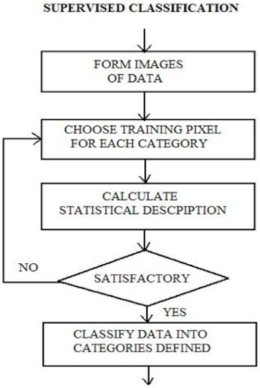
4.1. Supervised Classification for Change Detection

The supervised classification of remote sensing image data and the identification and placement of some land cover types, such as water, urban, and vegetation, are all known a priori through a combination of fieldwork, high-resolution image analysis, and personal experience. Compared to unsupervised classification, supervised classification has various advantages. For starters, because the classes are user-created, they adhere to the classification system. Second, using training data helps to enhance the ability to distinguish between classes. Finally, the procedure is more consistent and produces more precise findings.

4.1.1. Machine Learning Technique

The science of the computer modelling of learning processes is known as machine learning. It allows a machine to learn from existing facts or theories by employing inference procedures such as induction or deduction. Machine learning research has been conducted with differing degrees of enthusiasm over the years, utilizing various methodologies and focusing on various features and aims. The separability matrix containing the spectral distributions of probable classes in corresponding bands was used in this technique to develop a decision tree induction procedure for remotely sensed satellite data [15].

(A) 

Separability-Matrix-Based Decision Tree Induction

According to the splitting rule [15], a given collection of classes is divided into two subsets based on whether the separability is maximum or the amount of spectral overlapping between the two subsets is minimal. First, depending on the midpoint value, all the spectral classes are ordered in an increasing order. (Min + Max)/2 is used to obtain the midpoint. When just the upper diagonal elements are used when determining the threshold, the number of matrix computations is reduced. The threshold is obtained by finding the midpoint between the spectral distributions of the classes in the band where the separability is the greatest and the overlapping is the least. A node is created and labelled with the class number of the pure subset with only one class when a subset of classes becomes homogeneous. The splitting criterion is applied to a subset that has more than one class until it becomes purer.

The symbols used in the Algorithm 1 are:

• S—the set of the spectral distribution of classes with their class labels.
• S_L—the set of classes having distributions with range maximum or mid-point ≤ T.
• S_R—the set of classes having distributions with range minimum or mid-point T.
• n—the number of classes in the dataset.
• n_L—the number of classes in S_L.
• n_R—the number of classes in S_R.
• K—the number of spectral bands.
• M_k = ($m_{ij}^k$), (1 ≤ i ≤ n, 1 ≤ j ≤ n)—the separability matrix in band k.
• $C_{kl}^1$—the minimum range of spectral distribution in band k for class l.
• $C_{kl}^2$—the maximum range of spectral distribution in band k for class l.

• Input:
• S—the set of the spectral distribution of classes with their class labels.
• n—the number of classes in the dataset.
• K—the number of spectral bands.
• M_k = (m_ij^k), (1 ≤ i ≤ n, 1 ≤ j ≤ n)— the separability matrix in band k.

• Output:
• A decision tree classifier.

Algorithm 1 Separability-Matrix-Based Decision Tree Induction

Initialize the root by all the classes DTree ( N,S,n) Step 1: For each band 1 ≤ k ≤ K sort the spectral distributions with respect to the midpoint,       If n ≤ 2 and overlapping,          then construct the tree as in special       else        go to step 2. Step 2: For 1 ≤ k ≤ K, 1 ≤ i ≤ n, 1 ≤ j ≤ n             $M_k=\left\{\begin{array}{c}0 , if i=j\\ C_{kl}^1-C_{kl }^2, otherwise\end{array}\right.$ Step 3: case1: If $\exists$ b, r, c such that $m_{rc}^b$=          $\underset{1\le k\le K}{\max }\left\{\underset{1\le j\le n}{\max }\left\{\underset{i+1\le j\le n}{\min }\left\{m_{ij}^k/m_{ij}^k \ge 0 for all j\right\}\right\}\right\}$            Threshold(T) = $\frac{1}{ 2}\left\{C_{br}^2+C_{bc}^1\right\}$             BAND = b        go to step 4:           case2: If $\exists$ b, r, c such that $m_{rc}^b$ =            $\underset{1\le k\le K}{\max }\left\{\underset{1\le j\le n}{\max }\left\{\underset{i+1\le j\le n}{\min }\left\{m_{ij}^k/m_{ij}^k \ge 0\right\}\right\}\right\}$                T = T2 = $\frac{1}{2}\left\{C_{br}^2+C_{bc}^1\right\}$ Check whether the threshold T lies in any of the spectral range in the band b, except for the class distributions represented by r and c.              If yes, compute           EF2 = $\max \left\{\min \left\{\left|T-C_{bi}^1\right|, \left|T-C_{bi}^2\right|\right\} \forall \mathrm{class}i, i \ne r\mathrm{and}i \ne \mathrm{c},\mathrm{such}\mathrm{that}T ϵ \left(C_{bi}^1 ,C_{bi}^2\right)\right\}$        go to case 3:             if no go to step 4:        case 3: $m_{rc}^b$ = $\underset{i<k<K}{\max }\left\{\underset{i<j}{\max }\left\{m_{ij}^k\right\}\right\}$              T = T3 = $\frac{1}{2}\left\{C_{br}^2+C_{bc}^1\right\}$             BAND = BAND3 = b             EF3 = $\max \left\{\min \left\{\left|T-C_{bi}^1\right|, \left|T-C_{bi}^2\right|\right\} \forall \mathrm{class}i, i \ne r\mathrm{and}i \ne c,\mathrm{such}\mathrm{that}T ϵ \left(C_{bi}^1 ,C_{bi}^2\right)\right\}$             If EF2 $\le$ EF3 then T = T2 AND BAND = BAND2        go to step 4 step 4: Assign the threshold (T) & BAND to the node N. step 5: if $n_L\le 1$               then stop        else Dtree($N_L,S_L,n_L$)       If $n_R\le 1$              then stop      else  DTree($N_R,S_R,n_{R }$)

4.1.2. Training Data

After the adoption of the classification scheme, an image analyst may select training sites within the image that are representative of the classes of interest. If the environment from which the training data is collected is relatively homogeneous, it should be valuable. We generally apply geographical stratification during the preliminary stages for the geographic signature extension problem. At this time, all the important environmental factors that affect the geographic signature extension problem should be identified. Such environmental factors should be carefully added to the imagery, and the selection of the training data is based on the geographic stratification of these data. However, if the environmental conditions are homogenous, there is a significant reduction in the training cast and effort.

Each training site is composed of many pixels. The general rule is that if the training data are extracted from n bands, then the number of pixels of training data for each class collected is >10n. This is enough to calculate the variance–covariance matrices.

Each pixel in each training site is associated with a particular class (c) represented by an X_c measurement vector.

$$X_c=\left[\begin{array}{c}B{V}_{ij1}\\ B{V}_{ij2}\\ B{V}_{ij3}\\ .\\ .\\ .\\ B{V}_{ijk}\end{array}\right]$$

where BV_ijk is the brightness value for the i, jth pixel in band k.

The brightness values of each pixel in each training class in each band can then be analyzed statistically to yield a mean measurement vector, M_c, for each class:

$$M_c=\left[\begin{array}{c}{\mu }_{c1}\\ {\mu }_{c2}\\ {\mu }_{c3}\\ .\\ .\\ .\\ {\mu }_{ck}\end{array}\right]$$

where µ_ck represents the mean value of the data for class c in band k.

The measurement vector can also be analyzed to produce the covariance matrix for each class c.

$$V_c=V_{ckl}=\left[ \begin{array}{c}Co{v}_{c11} Co{v}_{c12}\dots Co{v}_{c1n}\\ Co{v}_{c21} Co{v}_{c22}\dots Co{v}_{c2n}\\ Co{v}_{c31} Co{v}_{c32}\dots Co{v}_{c3n}\\ \dots \\ \dots \\ \dots \\ Co{v}_{cn1} Co{v}_{cn2}\dots Co{v}_{cnn}\end{array}\right]$$

where Cov_ckl is the covariance of class c between bands k through l.

The positive spatial autocorrelation exists among pixels that are contiguous or close together [34]. It means the neighbor pixels have a high probability of having similar brightness values. The training data collected from the auto-correlated data are likely to have reduced variance. The goal is to collect non-auto-correlated training data. Unfortunately, most digital image processing systems do not offer this option in the training data-collection modules.

4.1.3. Optimum Band Feature Selection

Following the systematic collecting of training statistics from each band for each class of interest, a choice must be made about which bands best distinguish each class from the rest. Feature selection [35] is a term used to describe this procedure. The goal is to reduce the dimensionality (i.e., the number of bands to be processed) in the dataset by removing the bands that give redundant spectral information from the study. This reduces the cost of the digital picture categorization process, but it should not reduce its accuracy. Feature selection can be conducted using statistical and graphical analysis to establish the degree of class separability in the remote sensing training data.

(A) 

Spectral Values

Even if statistical techniques provide the information necessary to identify the most successful bands for classification based only on the statistic, the graphical method of feature selection does not provide fundamental knowledge of the spectral nature of the data. Many people who work in remote sensing are graphically literate by necessity, meaning that they can rapidly and readily interpret maps and graphs. A graphical display of statistical data is useful and necessary for a complete study of multispectral training data and feature selection. The mean, standard deviation (σ) is displayed in a bar graph spectral plot, which is one of the easy feature selection aids. This provides a clear visual representation of the degree of class separability for a single band.

4.2. Supervised Change Detection

The interpreter in supervised categorization knows ahead of time which classes, etc., are present. These are located on the image; the areas containing class examples are delimited (making them training sites), and a statistical analysis of the multiband data for each of these classes is undertaken. The goal of feature selection is to find the best multispectral bands for distinguishing one training class from another.

Instead of clusters, one can use class groupings with proper discriminating functions to separate each training class. When more than three bands are employed, more than one class may have identical spectral values, but this is improbable because distinct classes/materials rarely exhibit similar reactions over a large range of wavelengths. If more training data is required, it is gathered, and the classification algorithm is used. All the pixels not included in the training sites are then compared to discriminants produced from the training sites, and each is allocated to the class it is most similar to, forming a map of established classes. A set of signatures defines a training sample or a cluster as a result of the training. Each signature is associated with a class and is used in conjunction with a decision rule to assign a class to each pixel in the image file. Following the definition of signatures, the image’s pixels are sorted into classes based on the signatures using a classification decision rule and the data contained in the signature, which accomplishes the sorting of the pixels into different class values.

All classes of interest must be carefully selected and defined to correctly categorize the remotely sensed data into land use and/or land cover information. Geographical information, including the remote sensor data, is not precise. For example, there is gradual change in the interface of rivers and forests and many of the classification schemes are based on hard boundaries between the classes. Finally, there must be a general relationship between the classification scheme and the spatial resolution of the remote sensor system to provide information. The logical steps are presented in Figure 4 [36].

Supervised Post-classification Comparison.

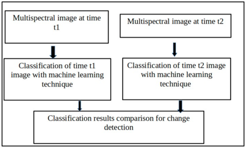
In post-classification change detection, the images are individually classified using any of the classification techniques, and then, the classification results are compared to determine the changes. In the supervised post-classification change detection technique, the machine learning technique is used to classify the remote sensing images. The accuracy of this method depends on the accuracy of the classification results on each image. A framework for the post-classification comparison is shown in Figure 5.

4.3. Change Detection Using Algebraic Technique

All the algorithms under the algebraic technique have a common characteristic of selecting thresholds to find out about the changed areas. Only changes greater than the identified threshold can be detected and can provide detailed change information. These methods are relatively simple, easy to implement and interpret, and straightforward. It is difficult to select a suitable threshold to identify the detailed change areas.

(A) 

Thresholding

If an image Img(x,y) contains light objects (change) on a dark background (no change), then these objects may be extracted using Equation (2) by a simple threshold value.

$$Img\left(x,y\right)=\left\{\begin{array}{c}1 Img\left(x,y\right)>T\\ 0 Img\left(x,y\right)\le T\end{array}\right.$$

(2)

where T is the threshold value that the analyst must provide experimentally or statistically. All the pixels that have changed are coded 1, whereas the background (which has not changed) is coded 0. To be meaningful, the best threshold level selection should be coupled with a priori knowledge of the scene or visual interpretation [37]. The image’s histogram can also be used to calculate the threshold values.

(B) 

Image Differencing

If both the images have almost the same radiometric characteristics, the subtraction results in zero values in the area having no change and negative or positive values in the area of change. Then, the results are stored in a new change image. Mathematically it may be expressed by Equation (1), here, BV_ijk is the brightness value for the i, jth pixel in band k.

After obtaining the difference image, it is necessary to divide it into two classes for classification: change and ‘no-change’. The pixels with radiance changes tend to cluster near the mean, while the pixels with no radiance change tend to cluster around the mean [38,39]. When two classes exist, one is substantially larger than the other and contributes so much to the histogram that it effectively covers and hides the presence of the other class, resulting in a unimodal distribution [19].

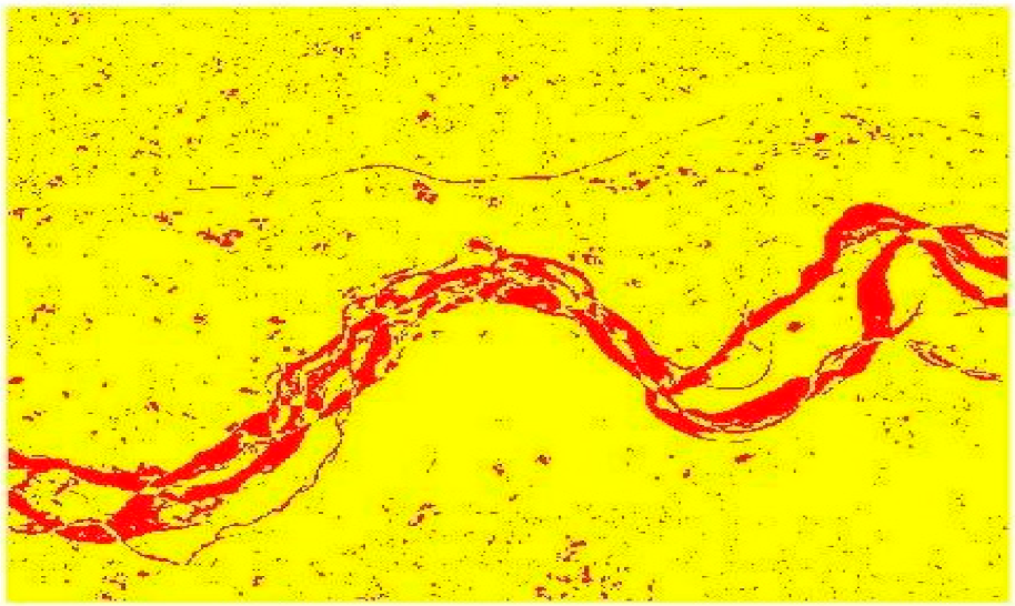
(C) 

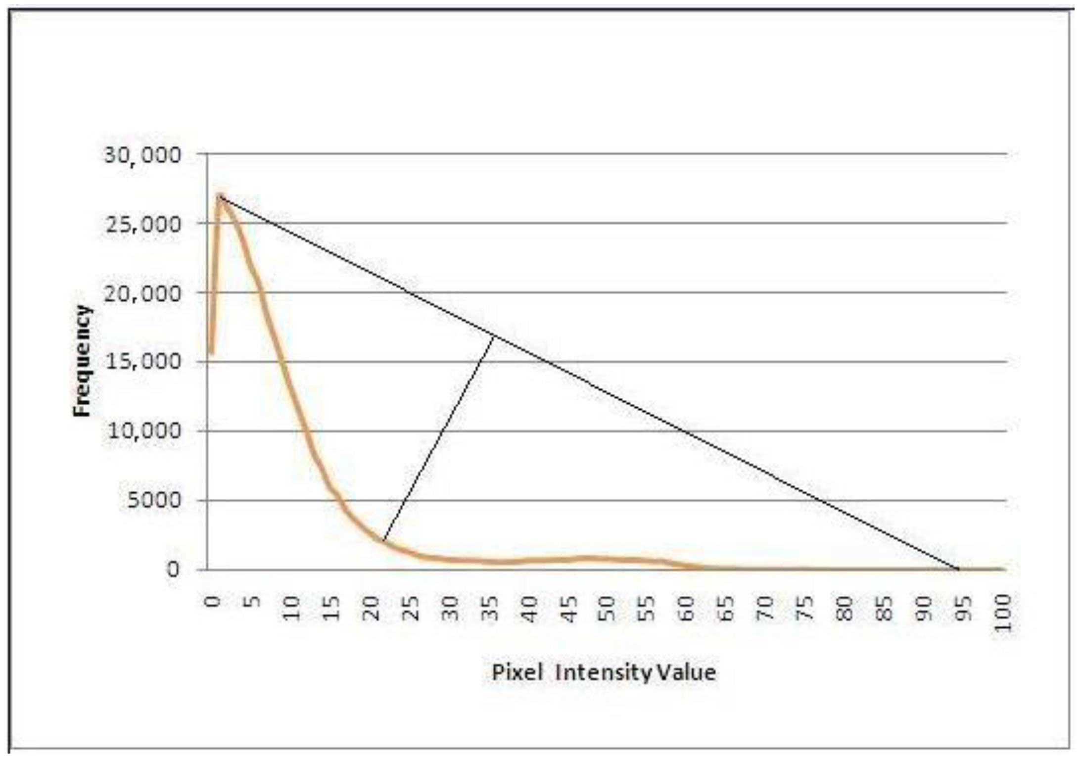
Corner Method

Rosin [19] was the first to propose this strategy. The image histogram is examined in this manner, and a threshold is chosen as the curve’s ‘corner’. The point on the curve with the greatest deviation from the straight line drawn between the curve’s endpoints is used to determine this threshold. The assumption is that the histogram is primarily unimodal, with a peak generated by a large number of pixels relating to modest levels of change and a long tail formed by a combination of processes, including noise, radiometric discrepancies, and pixels pertaining to significant change. Because it separates the peak from the tail, the curve’s ‘corner’ is a suitable threshold.

5. Experiments and Results

To carry out the experiment, the two images of the Delhi region have been used; they were obtained from Earth Explorer.

5.1. Machine Learning and Algebraic technique

This subsection provides a glimpse of the proposed machine learning and algebraic technique used for the experiments and results.

(A) 

Machine Learning Technique

(1)

The training samples for each class (water, vegetation, sand, and built-up) in each band were manually extracted from the first image to apply the decision tree classification algorithm using the separability matrix.

(2)

After selecting the sufficient number of training pixels for each class, the feature selection was performed by graphical method to reduce the complexity of the processing of the remotely sensed image.

(3)

A model was induced for classification using the decision tree induction algorithm using a separability matrix.

(4)

The first image is classified based on the induced model; then, the classifier is used to classify the second image.

(5)

Post-classification comparison was performed on both the images for calculation of the percentage change information.

(B) 

Algebra Technique

(1)

The changing image for both the images were calculated by the following Equation (3),

$$∆B{V}_{ijk}=B{V}_{ijk}\left(Img1\right)-B{V}_{ijk}\left(Img2\right)$$

(3)

(2)

A threshold was chosen by the corner method to classify the changing image into two classes, i.e., ‘change’ and ‘no-change’.

5.2. Dataset Description

To experiment with the Landsat Thematic Mapper, five images were used. It is geo-referenced data, which means that each pixel in the images has a corresponding geographic location on the earth. In this experiment, there are two images of the Delhi region, one from May 1998 and the other from May 2011. The images are available for free download from Earth Explorer [38]. From these images, using the Delhi shapefile, the area near the Yamuna River was extracted. Finally, we have two images of the same location at a different time, one from May 1998 and one from May 2011. The Landsat dataset used in our experiment is orthorectified, which means the dataset is corrected for perspective and relief errors.

Each image has seven bands, and the dimensions of each band are 641 rows and 502 columns. Each image has a total of 260,028 pixels, and the spatial resolution of each pixel is 30 × 30 meters. The instantaneous field of view of each pixel is 900 m². The total study area is 289,603.8 km². The description of the dataset is given in

Table 1. Description of data.

Zone	43 N
Projection	UTM
Ellipsoid	WGS-1984
Dautam	WGS-84
Bands	7
Spatial resolution	30 × 30 m
Rows	641
Columns	502
UL Geo	77°14′12.94″ E, 28°39′2.87″ N

and shown in Figure 6.

5.3. Experimental Details

A segment of images cropped from the images of the Delhi shape file, dated May 1998 and May 2011, were named Img-98 and Img-11. The experiments were carried out in Algorithm 1 using the implementation of the decision tree induction algorithm and using the separability matrix in the machine learning techniques and image differencing with the corner method in the algebraic method. Here, the extracted training samples are divided into four classes: water, vegetation, sand, and built-up. The number of training samples collected for the water class is 226, the vegetation class is 347, the sand class is 233, and the built-up class is 521 from Img-98. The spectral ranges of each class in each band for Img-98 were collected. Feature selection was performed with the bar graph spectral plots to select the optimum bands for classification. Here, band1, band4, and band5 were selected after the band reduction. The class-spectral-intensity ranges of the four classes in Img-98 are shown in

Table 2. Class-spectral-intensity range of training pixels.

	Water	Sand	Vegetables	Built-Up
Band 1	78–103	118–166	87–130	71–87
Band 4	20–63	64–96	43–109	63–105
Band 5	16–120	112–178	114–186	59–111

.

After the decision tree is modelled using the training pixels, it is applied to Img-98. In this algorithm, first the spectral classes are ordered in increasing order based on the values of their midpoints. The threshold value is calculated from the separability matrix for splitting the tree. Cross-validation was performed for the model selection. After selecting the model, it was applied to the second Img-11 for change detection.

(A) 

Cross-validation

The 10-fold cross-validation was performed to validate the model. From the training samples from each class, ten percent of the samples was set apart as validation data and 90 percent as training to induce the decision tree classifier. The model was then applied to the validation and testing samples. To evaluate accuracy as the evaluating parameter, the experiment is repeated for all the ten folds, yielding ten models, namely M_9-1, M_9-2, …, M_9-10. The number of testing samples for the water class is 65, the vegetation class is 143, the sand class is 74, and the built-up class is 118. The outcome of the 10-fold cross-validation in terms of the accuracy of the validation and test data is presented in

Table 3. Machine-Learning-based Models with Accuracy, with selected Model.

Folds	Validation Accuracy (V)	Testing Accuracy (T)	Average = (V + T)/2	Model Selection
M9-1	100	91.25	95.75	M2
M9-2	99.23	91.50	95.36	M3
M9-3	99.23	91.25	95.24	M4
M9-4	96.94	91.00	93.97
M9-5	96.18	91.75	93.96
M9-6	92.36	91.50	91.93
M9-7	93.89	91.50	92.69
M9-8	100	92.00	96.00	M1
M9-9	98.63	90.50	94.56
M9-10	99.23	91.25	95.24	M5

.

It may be observed that the maximum accuracy for the validation is 100%, while the minimum is 92.36%. The classification accuracy of the ten models on the test data ranges between 90.50–92.00%. Therefore, in order to help select good models, an average of the two was computed. The confusion matrices with their accuracy for the training and testing data are presented in (

Table 4. 1. Confusion matrix of one-to-five-fold cross-validation. 2. Confusion matrix of six-to-ten-fold cross-validation.

1
	Water					Urban					Sand					Vegetation					Error of Omission
	M9-1	M9-2	M9-3	M9-4	M9-5	M9-1	M9-2	M9-3	M9-4	M9-5	M9-1	M9-2	M9-3	M9-4	M9-5	M9-1	M9-2	M9-3	M9-4	M9-5	M9-1	M9-2	M9-3	M9-4	M9-5
Water	22	22	22	22	22	0	0	0	0	0	0	0	0	0	0	0	0	0	0	0	0	0	0	0	0
Urban	0	1	1	0	0	52	51	51	49	50	0	23	0	0	0	0	0	0	3	2	0	1.92	1.92	5.76	3.84
Sand	0	0	0	0	0	0	0	0	0	0	23	0	23	23	23	34	0	0	0	0	0	0	0	0	0
Vegetation	0	0	0	0	0	0	0	0	0	0	0	0	0	1	3	0	34	34	33	31	0	0	0	2.94	9.67
Error of Commission	0	4.34	4.34	0	0	0	0	0	0	0	0	0	0	4.16	11.53	0	0	0	8.33	6.06
2
Water							Urban					Sand					Vegetation					Error of Omission
	M9-6	M9-7	M9-8	M9-9	M9-10	M9-6	M9-7	M9-8	M9-9	M9-10	M9-6	M9-7	M9-8	M9-9	M9-10	M9-6	M9-7	M9-8	M9-9	M9-10	M9-6	M9-7	M9-8	M9-9	M9-10
Water	22	22	22	26	22	0	0	0	0	0	0	0	0	0	0	0	0	0	2	0	0	0	0	7.14	0
Urban	8	8	0	0	0	44	44	52	52	52	0	0	0	0	0	0	0	0	0	0	15.38	15.38	0	0	0
Sand	0	0	0	0	0	0	0	0	0	0	23	23	23	26	22	0	0	0	0	1	0	0	0	0	4.34
Vegetation	0	0	0	0	0	0	0	0	0	0	2	0	0	0	0	32	34	34	41	34	5.88	0	0	0	0
Error of Commission	26.66	26.66	0	0	4.34	0	0	0	0	0	8	0	0	0	0	0	0	0	4.65	2.85

and

Table 5. 1. Confusion matrix of testing data of one-to-five-fold cross-validation. 2. Confusion matrix of testing data of five-to-ten-fold cross-validation.

1
			Water				Urban					Sand					Vegetation					Error of Omission
	M9-1	M9-2	M9-3	M9-4	M9-5	M9-1	M9-2	M9-3	M9-4	M9-5	M9-1	M9-2	M9-3	M9-4	M9-5	M9-1	M9-2	M9-3	M9-4	M9-5	M9-1	M9-2	M9-3	M9-4	M9-5
Water	63	63	64	63	64	2	2	0	1	0	0	0	1	1	1	0	0	0	0	0	3.07	3.07	1.53	3.07	1.53
Urban	0	0	0	0	0	125	125	125	125	125	18	18	18	18	18	0	0	0	0	0	12.58	12.58	12.58	12.58	12.58
Sand	0	0	0	0	0	0	0	0	0	0	59	65	58	58	65	15	9	16	16	9	20.27	12.16	21.62	21.62	12.16
Vegetation	0	0	0	0	0	0	0	0	0	0	0	5	0	0	5	118	113	118	118	113	0	4.23	0	0	4.23
Error of Commission	0	0	0	0	0	1.57	1.57	0	0.79	0	23.37	26.13	24.67	24.67	26.96	11.27	7.37	11.94	11.94	7.37
2
-			Water				Urban					Sand					Vegetation					Error of Omission
-	M9-6	M9-7	M9-8	M9-9	M9-10	M9-6	M9-7	M9-8	M9-9	M9-10	M9-6	M9-7	M9-8	M9-9	M9-10	M9-6	M9-7	M9-8	M9-9	M9-10	M9-6	M9-7	M9-8	M9-9	M9-10
Water	63	64	64	63	63	1	1	0	2	2	1	0	1	0	0	0	0	0	0	0	3.07	1.53	1.53	3.07	3.07
Urban	0	0	0	0	0	125	125	125	125	125	18	18	18	18	18	0	0	0	0	0	12.58	12.58	12.58	12.58	12.58
Sand	0	0	0	0	0	0	0	0	0	0	65	59	61	56	59	9	15	13	18	15	12.16	20.27	17.56	24.32	20.27
Vegetation	0	0	0	0	0	0	0	0	0	0	5	0	0	0	0	113	118	118	118	118	4.23	0	0	0	0
Error of Commission	0	0	0	0	0	0.79	0.79	0	1.57	1.57	26.96	23.37	23.7	24.32	23.37	7.37	11.27	9.92	13.23	11.27					-

).

With the criteria for selecting the model(s) among the ten models, the average accuracy should be greater than 95 percent. Here, five models have been selected, and these are numbered as M₁, M₂, M₃, M₄, and M₅, as shown in Table 3.

5.4. Results

The experiments of classifying the pixels of two images were performed by applying the five models M₁, M₂, M₃, M₄, and M_5. The results in terms of the number of pixels in each class after classifying both the images, i.e., Img-98 and Img-11, are presented. Considering the variance in the outcome of all the five models, the average outcome for both images was computed as in

Table 6. Class-wise number of pixels identification using top five machine learning models.

	Img-98				Img-11
Model/Class	Water	Built-Up	Sand	Vegetation	Water	Built-Up	Sand	Vegetation
M1	26,979	67,761	13,481	211,279	31,603	98,011	20,561	169,325
M2	22,752	92,997	10,317	193,434	25,612	130,406	15,698	147,784
M3	25,909	81,033	14,800	197,758	29,935	115,242	22,642	151,681
M4	28,537	62,149	9035	219,779	34,175	90,407	13,239	181,679
M5	23,975	82,967	10,369	202,189	27,401	117,776	15,727	158,596
Average	25,630	77,381	11,600	204,887	29,745	110,368	17,573	161,814

and

Table 7. Change computation table based on machine-learning-based models accuracy.

Class	Img-98	Img-11	(Img-11–Img-98)	Percentage Difference
Water	25,630	29,745	4115	16.05
Built-up	77,381	110,368	32,987	42.62
Sand	11,600	17,573	5973	51.49
Vegetation	204,887	161,814	−43,073	(21.02)

and exhibits the class-wise average number of pixels of Img-98 and Img-11 in columns 1 and 2. The third column presents the difference in the number of pixels classified in Img-98 and img-11 corresponding to each class—water, built-up, sand, and vegetation. The fourth column presents the percentage change. The false color code of the outcome of the decision tree classifier using the separability matrix was generated. The red color is for the water class, the green color is for the built-up class, the blue color is for the sand class, and the yellow color is for the vegetation class. The outcome plot decision tree classifier using the separability matrix is presented in Figure 7.

In the algebraic technique, the change image matrix was calculated by the difference of the intensity values of Img-98 and Img-11. These images are shown in Figure 8. To find out the threshold value, the corner method was implemented. The histogram of the change image matrix was plotted and is shown in Figure 7.

The x-axis of the histogram represents the intensity value of the pixels, and the y-axis represents the number of pixels corresponding to the intensity value.

A straight line was drawn between the peak and the lowest point in the curve. The perpendicular distance between the point and the line was calculated from each point in the curve. The point with the maximum distance from the line was selected, and the corresponding x coordinate was chosen as the threshold to classify the change image matrix into two classes (change and no-change).

The intensity values which are greater than the computed threshold values are classified as change; otherwise, they are no-change. The false color image of the outcome of the image differencing is shown in Figure 9. The red color indicates the changed pixels, and the yellow color indicates the unchanged pixels.

5.5. Analysis

From all the experimental results, as presented in Table 3, Table 6 and Table 7, it is observed that changes in the two image segments, Img-98 and Img-11, were detected. Table 6 displays the number of changed and unchanged pixels and the percentage of change for each class.

From the experimental results, as presented in Table 3, it is observed that for fold M_9-8 the validation accuracy and the testing accuracy are the highest. So, this has been named as the first model (M₁). The validation accuracy is highest in the first fold M_9-1, but the testing accuracy is not the highest. Unlike M_9-1, the validation accuracy is not the highest in the second fold, but the testing accuracy is more than that of the first one. So, to find out the models with a good overall accuracy, the average of the validation accuracy and testing accuracy has been considered. Here, five models M₁, M₂, M₃, M₄, and M₅ have been selected to classify the images Img-98 and Img-11.

The experimental results presented in Table 6 show that the number of pixels for each class in Img-98 and Img-11 has been calculated by applying the five models selected from Table 3. The average number of pixels for each class has been calculated for the change detection.

From the experimental results, as presented in Table 7, it may be observed that from Img-98 to Img-11 the water has increased by 16%, the built-up area/built-up has increased by 42.69%, the bare earth/sand area has increased by 51.49%, and there is a decrease in vegetation area by 21%.

In the image differencing, the threshold for finding the change has been calculated, and its value is 21. The intensity values less than 21 are classified as unchanged, and those greater than or equal to 21 are classified as changed. The number of changed pixels using this method is 41,297, and the number of unchanged pixels is 280,485.

(A)

Comparison of post-classification and algebraic technique

For the post-classification comparison, the number of change pixels for each class can be calculated from Table 7. However, in the case of the algebraic technique, only the number of pixels can be calculated, which is 41,297. In the case of the algebraic technique, it is difficult to calculate the threshold, but in the post-classification comparison, as the training samples have been selected, its accuracy is reliable compared to the algebraic technique. In the post-classification comparison, the number of changed pixels is around 86,148, and for image differencing, it is 41,279. However, the image differencing with the corner method to identify the threshold does not perform well in the two images of the Delhi region, one from May 1998 and the other from May 2011, to identify the change and unchanged pixels compared to the decision tree classifier.

6. Conclusions and Future Work

This research aims to improve the classifier accuracy of the machine learning techniques in post-classification comparison and compare it with the algebraic techniques for change detection in remote sensing images. In supervised learning, the size of the training samples is much larger compared to the test data. However, in the case of the remote sensing image data, the size is smaller compared to the test data. Therefore, the study aimed to review the training of the classifiers to improve the classifier accuracy of the machine learning techniques.

The experimental result shows that machine learning techniques can be applied to change the detection process to make it automatic. The result of the cross-validation shows that the accuracy can be increased by proper training and testing the samples. The experimental results show that the post-classification comparison using the machine learning techniques performs well over the image differencing of the algebra technique.

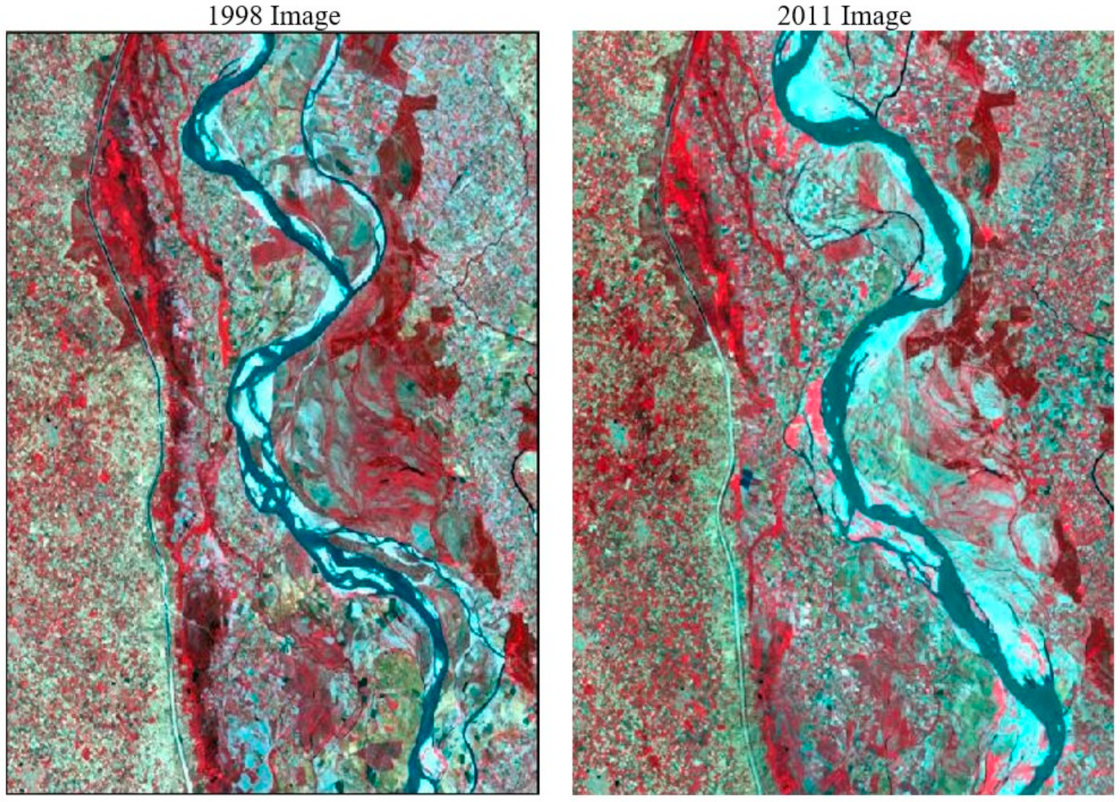
The post-classification comparison-based change detection technique quantitatively indicates that in the study area between 1998 and 2011, the urban area has increased, the water area has increased, the bare earth/sand has increased, and the vegetation cover has decreased. At the same time, some pixels from the vegetation may have changed to bare earth/sand or built-up area or water.

As the ground truth is outside the scope of work, the accuracy assessment has not been conducted. However, this result is consistent with common trends in urban development. The limitation of this work is that the proposed technique is based on a decision tree that is little bit old nowadays, and from dataset point of view, we have applied the proposed technique on a limited dataset. Computationally, time analysis was not performed before the using of the algorithms. We would like to analyze these drawbacks in future.

The future work of this research work can be extended to:

1

In the machine learning techniques, the decision tree is used here. Some other machine learning techniques, such as the candidate elimination algorithm, the covering algorithm, etc., can be used for classification for post-comparison change detection.

2

In this study, no spatial information has been considered. The spatial features of the pixels can be incorporated while classifying the image.

3

In this study, pixel-wise classification has been performed. The object-based computation can also be applied where the whole image is first divided into different regions, and then, those regions are classified.

4

In image differencing, to calculate the threshold value, some probabilistic methods can be used.