A Multi-Scale Multi-Task Learning Model for Continuous Dimensional Emotion Recognition from Audio

Abstract

Due to the advantages of many aspects of the dimensional emotion model, continuous dimensional emotion recognition from audio has attracted increasing attention in recent years. Features and dimensional emotion labels on different time scales have different characteristics and contain different information. To make full use of the advantages of features and emotion representations from multiple time scales, a novel multi-scale multi-task (MSMT) learning model is proposed in this paper. The MSMT model is constructed by a deep belief network (DBN) with only one hidden layer. The same hidden layer parameters and linear layer parameters are shared by all features. Multiple temporal pooling operations are inserted between the hidden layer and the linear layer to obtain information on multiple time scales. The mean squared error (MSE) of the main and the secondary task are combined to form the final objective function. Extensive experiments were conducted on RECOLA and SEMAINE datasets to illustrate the effectiveness of our model. The results for the two sets show that even adding a secondary scale to the scale with optimal single-scale single-task performance can achieve significant performance improvements.

1. Introduction

Artificial intelligence technology is a hot topic of research and discussion in current society. Researchers have developed different machine learning models to deal with different problems, such as [1] developing regularized extreme learning machines to train multi-label neural network classifiers. Various machine learning models are also widely used in various aspects of production and life to improve the efficiency of our work and improve the convenience and comfort of life. For example, ref. [2] proposed a machine learning method to find a set of clinical indicators predicting poor prognosis and morbidity from the blood of COVID-19 patients, so that clinicians can make judgments on patients more quickly and easily.

Accurate emotion recognition plays a vital role in daily human communication. Therefore, this is the basis for building a natural, friendly, and harmonious human–computer interaction. Since human beings express emotions through multiple channels (voice, facial expressions, body gestures, physiological signals, etc.), emotion recognition can also be performed from one or more modalities. In recent years, researchers have used various modalities and combinations for emotion recognition. In ref. [3], a novel, deep neural architecture is proposed to extract feature representations from heterogeneous acoustic feature groups, enabling category emotion recognition. Ref. [4] uses CapsNet for dimensional emotion category recognition from multi-band EEG signals. Ref. [5] uses a transformer-based cross-modal fusion with the EmbraceNet architecture to achieve multi-modal emotion recognition based on audio, video and text modalities. As there is a large gap between acoustic features and human emotion, audio-based emotion recognition has always been a challenging task. In this paper, we focus on speech-based emotion recognition.

In the field of emotion recognition, the most commonly used emotion model is the category model. However, there is another dimensional emotion model, which has attracted increasing attention in recent years due to its many advantages, including its ability to distinguish subtle emotions, describe the evolution of emotions, and so on [6]. In the dimensional emotion space, emotion is represented as a point in a multidimensional space, and each dimension measures a particular property of emotion [7]. For example, “valence” is the measure of pleasantness, “arousal” is the measure of activation, “dominance” is the measure of attention, and so on [7]. As the two dimensions of “arousal” and “valence” can represent most emotions [8], most researches on dimensional emotion recognition are based on these two dimensions [9,10].

In this paper, we focus on continuous dimensional emotion recognition based on the “valence-arousal” space from audio, which aims to predict the continuous valence and arousal values at every moment (frame), making it a sequential regression problem [9].

According to our daily experience, emotional judgments on a larger timescale tend to be more fuzzy and conceptual, but the accuracy of assessments will be higher. Emotional judgments on a smaller timescale will be more refined, but the accuracy is more likely to be affected by various factors. During dimensional emotion recognition, the standard method of emotion recognition on a particular timescale is the addition of sliding windows to features and labels. By calculating several functionals (mean, min, max, etc.) on the features and calculating the average value of the labels in the window, new samples and corresponding labels are obtained. Based on these samples and corresponding labels, continuous dimensional prediction can be realized. Ringeval et al. [11] investigate the influence of different window sizes on emotion prediction performance. The results show that an appropriate window size can achieve a trade-off between information loss and noise reduction, making it better than direct, frame-by-frame emotion recognition. Additionally, different emotional characteristics can be obtained at different timescales [12]. Jonathan et al. [12] propose a fusion method that utilizes the outputs of different classifiers trained on various timescales to achieve emotion classification, and showed a significant improvement in unweighted accuracy. However, directly adding windows to features is inefficient and limited to capturing temporal dynamic information. Inspired by the convolutional neural network, which inserts a feature pooling layer between two convolutional layers to obtain hierarchical spatial information, Hamel et al. [13] propose a multi-time-scale learning model (MTSL), which adds a temporal pooling layer to the output of a network to obtain hierarchical temporal information. Chao et al. [14] introduce this method into continuous dimensional emotion recognition and achieve a competitive performance. The temporal pooling layer is behind a hidden layer so that the pooled features dynamically change during training. Therefore, pooled features are more expressive than the feature functions in a window, and it also improves the diversity of input features in the next layer [15]. Since then, this method has been used in many works (e.g., [15,16]). In previous work, emotion recognition only relies on one temporal pooling and does not fully utilize information on different timescales. In this paper, we introduce a novel method to use multiple temporal pooling results for continuous dimensional emotion recognition.

Multi-task learning can learn shared representations from different tasks to improve the generalization ability of the system [17]. This is widely used in the recognition problem, emotion recognition is no exception. Wang et al. [18] propose a two-stage, multi-task learning structure, which uses categorical representations to improve dimensional representations and simultaneously estimate valence and arousal. Xia et al. [19] apply multi-task learning to leverage activation and valence information for acoustic categorical emotion recognition. Kollias et al. [20] set up and tackle multi-task learning for emotion recognition, as well as facial image generation.

In this work, to make use of information on different timescales, we propose a multi-scale multi-task (MSMT) learning framework to implement continuous dimensional emotion recognition. We use the temporal pooling technique to utilize the information on a timescale. Our experiments and previous experiments [14] show that more hidden layers before the temporal pooling layer cannot significantly improve the performance of dimensional emotion recognition. Thereby, we construct an MSMT model based on the deep belief network (DBN) with only one hidden layer. The network is first unsupervised and pre-trained, then fine-tuned in a supervised manner. The MSMT learning is only performed in the fine-tuning stage. All features pass through the same hidden layer, then are pooled by pooling layers with different pooling sizes, and finally pass through the same linear layer with tanh activation. The MSEs of the main and secondary scales are combined to form the objective function.

The network we constructed can simultaneously use feature information and label information from multiple timescales. When training the network to realize dimensional emotion recognition on one timescale, by learning the dimensional emotion recognition task on another timescale, the network can obtain information on multiple scales, which is expected to improve the recognition performance. Extensive experiments were conducted on the RECOLA dataset and the SEMAINE dataset to illustrate the effectiveness of the model. The experimental results show that even if the scale with optimal single-scale single-task (SSST) performance is used as the main scale, and the scale with poor SSST performance is used as the secondary scale, there is still a significant performance improvement on the basis of the original optimal performance.

2. Deep Belief Network

In this paper, we use the deep belief network (DBN) composed of only one Restrict Boltzmann Machine (RBM) to construct our model. The difference between this DBN, with only one hidden layer, and RBM is the only training process. After unsupervised pre-training RBM, the network needs to be fine-tuned in a supervised manner.

An RBM is an undirected graphical probability model with one visible layer and one hidden layer, and there is no connection within the layers. Usually, RBM is used to model binary vectors. In view of the audio features being real-valued, Gaussian-RBM is used in this work, which is a variant of RBM. A Gaussian-RBM has a real valued stochastic variable (denoted as $\mathbf{v}\in R^D$) and a binary stochastic hidden variable (denoted as $\mathbf{h}\in {\{0,1\}}^F$), where $D,F$ are the number of nodes in the visible layer and the hidden layer, respectively. The energy function is defined as

$$E(\mathbf{v},\mathbf{h})=\frac{1}{2}{(\mathbf{v}-\mathbf{b})}^T{\Lambda }^2(\mathbf{v}-\mathbf{b})-{\mathbf{v}}^T\Lambda W\mathbf{h}-{\mathbf{a}}^T\mathbf{h},$$

(1)

where $W$ is the connection weight matrix between the visible and hidden layer, $\mathbf{a},\mathbf{b}$ are the bias vectors for the hidden and visible layers, respectively, and $\Lambda =diag(1/{\sigma }_1,\cdots ,1/{\sigma }_D)$ with ${\sigma }_i(i=1,\cdots ,D)$ is the standard deviation of the visible unit. The density function of $\mathbf{v}$ is

$$P(\mathbf{v})=\frac{1}{Z}\cdot {\displaystyle \sum _{\mathbf{h}}^{}\exp (-E(\mathbf{v},\mathbf{h}))},$$

(2)

where $Z$ is the partition function. The components of the visible variable $\mathbf{v}$ are independently conditioned on hidden variables and vice versa. The conditional distributions of each component in visual variable and hidden variable are

$$P(h_j=1|\mathbf{v})=g(\mathbf{v}\Lambda W_{\cdot j}+a_j),j=1,\cdots ,F,$$

(3)

$$v_i|\mathbf{h}\sim N(b_i+{\sigma }_i{W}_{i\cdot }\mathbf{h},{\sigma }_i^2),i=1,\cdots ,D,$$

(4)

where $W_{i\cdot },W_{\cdot j}$ are the ith row vector and jth column vector of $W$, respectively, $g(x)=1/(1+\exp (-x))$ is the logistic function, $N(\mu ,{\sigma }^2)$ represents the Gaussian distribution with expectation, and variance are and ${\sigma }^2$, respectively [21]. The learning task is to find parameters $W,a$ and $b$ to maximize the log-likelihood function. The stochastic gradient ascent algorithm is usually used to achieve this task. For a given training vector $\mathbf{v}$, the derivatives of the log-likelihood with respect to $W$, $a$ and $b$ are

$$\begin{array}{l}\frac{\partial \log P(\mathbf{v})}{\partial W}=<\mathbf{v}\Lambda {\mathbf{h}}^T{>}_{P(\mathbf{h}|\mathbf{v})}-<\mathbf{v}\Lambda {\mathbf{h}}^T{>}_{P(\mathbf{v},\mathbf{h})},\\ \frac{\partial \log P(\mathbf{v})}{\partial a}=<\mathbf{h}{>}_{P(\mathbf{h}|\mathbf{v})}-<\mathbf{h}{>}_{P(\mathbf{v},\mathbf{h})},\\ \frac{\partial \log P(\mathbf{v})}{\partial b}=<\mathbf{v}{\Lambda }^2{>}_{P(\mathbf{h}|\mathbf{v})}-<\mathbf{v}{\Lambda }^2{>}_{P(\mathbf{v},\mathbf{h})},\end{array}$$

(5)

where $<\cdot {>}_{P(\cdot )}$ is the expectation under the distribution $P(\cdot )$. As obtaining an unbiased sample from the distribution $P(\mathbf{v},\mathbf{h})$ is very difficult, a Contrastive Divergence (CD)-based learning algorithm is usually used to effectively approximate the change in parameters in each iteration [22]. Although the variance of each visual unit can be determined by learning, this is difficult when using CD [22]. In our work, we set ${\sigma }_i^2=1$, and normalize each component of the features to obtain unit variance.

After pre-training, the Gaussian-RBM is used to initialize a feed-forward network. In fact, the pre-training process is not necessary. Without the pre-training process, we can also obtain results through the random initialization of the forward network. However, the effect of random initialization depends entirely on luck, which is sometimes very good and sometimes very poor. Through the pre-training process, the network parameters can be adjusted to a more sensitive position, so that the final tuning result is more stable. Therefore, in all our experiments, a pre-training process was used before fine-tuning.

Since the value range of our dimensional emotion label is $[-1,1]$, to supervise the fine-tuning of this feed-forward network, a linear layer with tanh activation function is added on top of the hidden layer $\mathbf{h}$. Let $W_l$ and $b_l$ be the weight matrix and the bias of the linear layer; the output of the network is $y=\tanh ({\mathbf{h}}^T{W}_l+b_l)$. Then, the standard backpropagation algorithm can be used to minimize the MSE between the predicted value and the reference value. After fine-tuning, the network can be viewed as a regressor, and the output of the linear layer is the final predicted value.

3. Multi-Scale Multi-Task Framework for Continuous Dimensional Emotion Recognition

The perception and description of emotion show different characteristics on different timescales [12]. Multi-task learning can obtain necessary information from the learning of related tasks, thereby improving the generalization ability of the main-task learning [19]. Here, we use the idea of multi-task learning to build a multi-scale multi-task (MSMT) learning framework to make full use of information on multiple timescales to improve the performance of continuous dimensional emotion recognition.

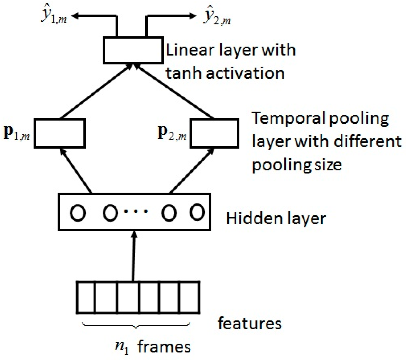
The proposed MSMT learning framework is illustrated in Figure 1. The framework is constructed by a DBN with only one hidden layer. Multiple pooling layers with different pooling sizes are built on the hidden layer, followed by the same linear layer. The hidden parameters are initialized using unsupervised Gaussian-RBM pre-training. Suppose we intend to use the information from two timescales $n_1$ and $n_2$ (frames) to achieve continuous dimensional emotion recognition and $n_1>n_2$. During fine-tuning, for a given frame $m$ ($m$ represents both the name and index of this frame), the features of $n_1$ consecutive frames centered on $m$ (from frame $m-\mathrm{floor}(\frac{n_1-1}{2})$ to frame $m+\mathrm{ceil}(\frac{n_1-1}{2})$) are input to the network. All features share the same hidden parameters. The temporal pooling operations with timescales $n_i(i=1,2)$ (frames) centered on frame $m$ are applied to the output of the hidden layer. Although there are many pooling methods, we chose the most commonly used mean pooling here. Suppose the hidden layer output of frame $l$ is $\mathbf{h}(l)$, and the pooled features obtained using pooling sizes $n_i(i=1,2)$ are ${\mathbf{p}}_{i,m}(i=1,2)$; then,

$${\mathbf{p}}_{i,m}={\displaystyle \sum _{l=m-\mathrm{floor}(\frac{n_i-1}{2})}^{m+\mathrm{ceil}(\frac{n_i-1}{2})}\mathbf{h}(l)},i=1,2.$$

(6)

Next, the pooled features are input to a linear layer with tanh activation function. The pooled features with different pooling sizes share the same linear layer parameters. Let ${\widehat{y}}_{i,m}(i=1,2)$ represent the predicted values obtained under these two timescales; then,

$${\widehat{y}}_{i,m}=\tanh ({\mathbf{p}}_{i,m}{W}_l+b_l),i=1,2.$$

(7)

where $W_l$,$b_l$ are the weight matrix and the bias of the linear layer. Finally, the two predictions are combined to update the hidden and linear parameters.

We apply the same pooling operation as we did for the hidden output to the labels centered on frame $m$, and obtain the reference labels $y_{i,m}(i=1,2)$ of frame $m$ corresponding to the two timescales $n_i(i=1,2)$. We use the MSE between the predicted values and the reference values on the training subset as the loss function. Suppose there are $N$ frames in the training subset; then,

$$L_i=\frac{1}{N}{\displaystyle \sum _{m=1}^N{({\widehat{y}}_{i,m}-y_{i,m})}^2},i=1,2.$$

(8)

We choose the prediction under one timescale (assumed to be $n_1$) as the main task, and the prediction under other scales (assumed to be $n_2$, here) as the secondary task. Therefore, the objective function is

$$L=L_1+\alpha \cdot L_2,$$

(9)

where the function of parameter $\alpha$ is to control the role played by the secondary task in multi-task learning. When this objective function is minimized, the prediction errors based on these two timescales are simultaneously minimized. With the help of secondary tasks, the performance of the system’s continuous dimensional emotion prediction is expected to improve.

4. Experiments and Results

4.1. Dataset and Features

We used the audio data in the RECOLA database and the SEMAINE database to evaluate the effectiveness of our model [23].

4.1.1. RECOLA

There are 23 publicly available, five-minute audio recordings with continuous arousal and valence annotations (every 40 ms) in the RECOLA dataset. The dataset was used for several challenges (e.g., AVEC’15 [24], AVEC’16 [25], AVEC’18 [26]). We used the same train/development/test split as in these challenges. Each of the three sets contains 9 recordings. However, the recordings in the test set (we refer to them as the test1 set) are not included in the 23 publicly available recordings. We had no annotations for these 9 audio recordings, so they were only used in the unsupervised pre-training stage. There are five additional recordings (the names of the corresponding recordings are P17, P43, P48, P58, P62) in the RECOLA database, which were not used in any challenges. We used these recordings (we refer to them as the test2 set) to evaluate the generalization of our model.

The arousal and valence annotations in the RECOLA database were assigned at a 40-ms frame rate by six gender-balanced, French-speaking assistants using the ANNEMO toolkit [23]. In our experiments, we used the same procedure as was used in the AVEC’16 challenge to obtain the ground truth labels. Firstly, the annotations from each rater are centered to the weighted mean (weighted by their respective agreement) value of all raters. The agreement is measured by the CCC. Then, the six centered annotations are averaged to obtain the ground truth labels [25,27].

4.1.2. SEMAINE

The currently publicly available data in SEMAINE were obtained in the Solid SAL scenario, where a person plays the role of a machine “Operator” to communicate with “User”. This dataset was also used for several challenges (e.g., AVEC’11 [28], AVEC’12 [29], etc.). To facilitate comparison, we used the same train/development/test split as was used in these challenges. The three sets contained 31, 32, 32 videos of varying lengths, respectively. All these videos were annotated with four dimensions (i.e., arousal, valence, expectation, and power) by 2 to 8 annotators, at the frame rate of 49.979. The processed labels were given in the database as the ground truth, and we used these labels directly.

4.1.3. Features and Metric

We used the extended Geneva Minimalistic Acoustic Parameter Set (eGeMAPS), which contains 88 parameters [30], as the audio features, in accordance with the AVEC’16 challenge. The features were extracted every 40 ms and 20 ms for RECOLA and SEMAINE dataset, respectively, by the openSMILE toolkit [31] based on the eGeMAPS configuration file, with different window sizes for different emotion dimensions (4 s and 6 s for arousal and valence, respectively). The eventual dimension of the features was 88.

The Concordance Correlation Coefficient (CCC) was used to evaluate our model. The definition of the CCC of two sequences was [25]

$${\rho }_c=\frac{2\rho {\sigma }_x{\sigma }_y}{{\sigma }_x^2+{\sigma }_y^2+{({\mu }_x-{\mu }_y)}^2},$$

(10)

where ${\sigma }_x{}^2$,${\sigma }_y{}^2$ are the variances of two sequences $x$ and $y$, ${\mu }_x$, ${\mu }_y$ are the corresponding means, and $\rho$ is the Pearson correlation coefficient between the two sequences.

Since many results on the SEMAINE set were measured by Pearson Correlation coefficient (PCC), we also gave the PCC results of the SEMAINE dataset.

4.2. Data Processing

In our experiment, the data of the two datasets were processed in the same way. Since different components in the features have different value ranges, it was necessary to normalize the features. In our work, during unsupervised pre-training, we set the variance of each visual unit to 1. Therefore, the features were first linearly normalized to [−1,1], then scaled to unit variance. During fine-tuning, the features were normalized with z-score to zero mean and unite variance.

To compensate for the delay in the annotations, as in [10], we shifted the features backward rather than shifting the labels forward. To estimate the annotation delay for each emotion dimension, in accordance with [32], we calculated the CCC between each component of the delayed features and the corresponding labels, then averaged the CCCs over the entire training set. We continuously increased the delay time (represented by the number of frames) from 0 by step 1. If there was no improvement over the best average CCC after 10 iterations, the corresponding delay time was set as the annotation delay. The delays for the arousal and valence dimensions on the RECOLA dataset, calculated in this way, were 69 and 95, respectively. For the SEMAINE dataset, the results were 401 and 196 for the arousal and valence dimensions, respectively.

4.3. Experimental Setup

We referred to the model in Figure 1, with parts ${\mathbf{p}}_{2,m}$ and ${\widehat{y}}_{2,m}$ removed, as the single-scale single-task (SSST) model. In this paper, to illustrate the effectiveness of our model, we first used the SSST model to perform continuous dimension emotion recognition. We investigated the influence of different temporal pooling sizes on recognition performance. When using the MSMT model, we chose the learning on the timescale with the best performance in SSST recognition as the main task, and the learning on other time scales as the secondary task, to study the learning of the secondary task’s promoting effect on the learning of the main task.

In our work, the training of both the SSST model and MSMT model was divided into two stages: the pre-training stage and the fine-tuning stage. To facilitate comparison, the same parameters and criteria were used in all model training. In the pre-training stage, since no label information was required, there is not much data in RECOLA dataset, so all 27 recordings in the training, development, and test1 sets were used for pre-training. However, for experiments on SEMAINE dataset, only the data in the training set was used for pre-training. The number of hidden nodes was empirically set to 20. The connection weights were initialized with values from a truncated normal distribution, with a mean of 0 and a standard deviation of 0.01, and the biases were initialized with 0. The learning rate was set to ${10}^{-3}$, training batch size was set to 100, the number of steps for Gibbs sampling was set to 10, and the number of training epochs was set to 10. Momentum and weight decay were also used: the momentum was set to 0.5, and the weight-cost coefficient was set to 0.0001.

In the fine-tuning stage, only the training set was used for model training. The models were optimized by Adam algorithm with a learning rate of 0.1, and the batch size was set to 100. To avoid overfitting, the development set was used to implement the early stopping strategy. The analysis and selection of hyperparameters (pooling size, the secondary task coefficients, etc.) were based on the performance on the development set. Finally, the models were tested on the test set (for experiments on RECOLA dataset, refered to test2 set). All our experiments were performed 5 times, and the average results of these experiments were used for comparison and analysis. All our systems were built on Tensorflow and used one GPU to accelerate training.

4.4. Experimental Results

4.4.1. SSST Learning Results

In our work, the SSST model was first used to study the impact of different timescales on the performance of continuous dimensional emotion recognition and select an appropriate pooling size as the main task. Experiments were carried out on two dimensions, namely, the arousal dimension and valence dimension.

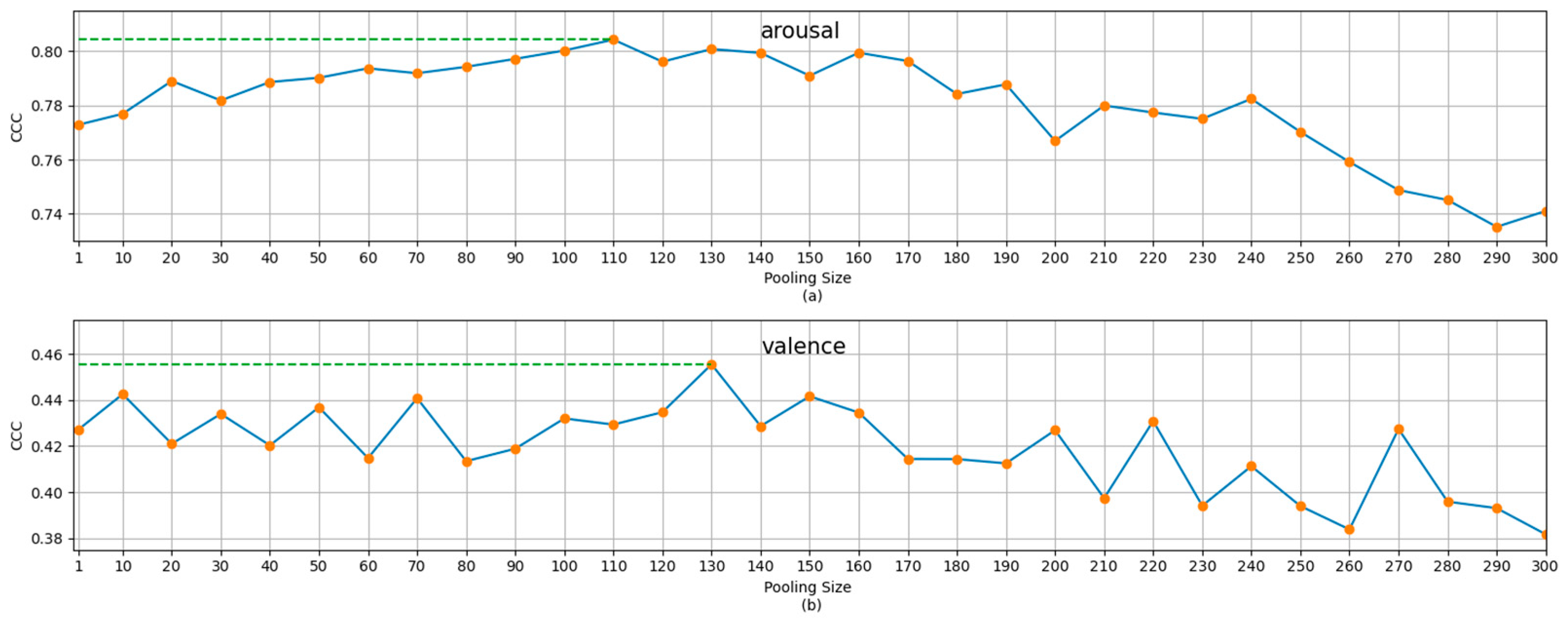
For experiments on RECOLA datasets, we increased the temporal pooling size from 10 (frames) to 300 (frames), in steps of 10 (frames). The results for the development set for the arousal and valence dimensions are shown in Figure 2, where the pooling size of 1 means no temporal pooling operation was used. The results for the development set and the test2 set for pooling size 1, and the best pooling size (determined based on the results on the development set), are also shown in

Table 1. The SSST recognition results (measured by CCC) on the development subset and the test2 subset of the RECOLA dataset for pooling size 1 and the best pooling size (determined based on the results on the development).

Pooling Size	Arousal		Pooling Size	Valence
	Development	Test2		Development	Test2
1 (no temporal pooling)	0.773	0.653	1 (no temporal pooling)	0.427	0.471
110	0.804	0.673	130	0.456	0.508

as the comparison baseline for the following MSMT results.

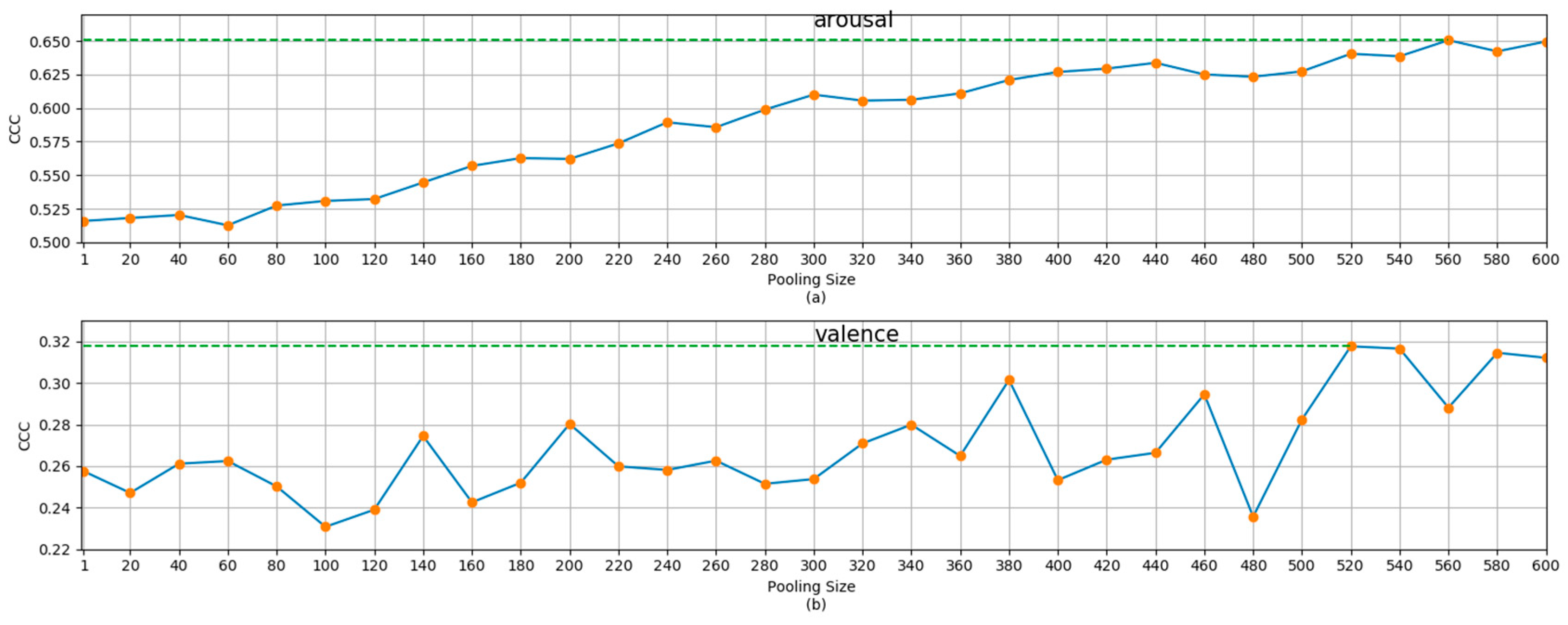
For the SEMAINE dataset, we increased the temporal pooling size from 20 (frames) to 600 (frames). The results for the development set for the arousal and valence dimensions are shown in Figure 3. As above, a pooling size 1 means no temporal pooling operation was used. The results for the development set and the test set for pooling size 1, and the best pooling size (determined based on the results for the development set), are also shown in

Table 2. The SSST recognition results (measured by the CCC) for the development subset and the test subset of the SEMAINE dataset for pooling size 1 and the best pooling size (determined based on the results on the development).

Pooling Size	Arousal		Pooling Size	Valence
	Development	Test		Development	Test
1 (no temporal pooling)	0.516	0.373	1 (no temporal pooling)	0.257	0.042
560	0.650	0.433	520	0.318	0.080

.

From the results in Figure 2 and Figure 3, Table 1 and Table 2, it can be seen that the temporal pooling operation has the ability to improve the recognition performance of the arousal dimension or the valence dimension. From Figure 2 and Figure 3, we can also see that as the pooling size increased, the recognition performance first increased and then decreased. This trend is particularly clear for the results for the RECOLA set. This is consistent with the argument in [11]. With the increase in the pooling size, the impact of noise interference reduces, and the context information that can be used increases, so the recognition performance improves. However, at the same time, with the increase in pooling size, the detailed information decreases, and the description of emotion becomes fuzzy and conceptual. Therefore, when the advantages and disadvantages reach a balance, the recognition performance begins to decline. A reasonable guess is that large-scale continuous dimensional emotion recognition can be improved with the help of small-scale emotion recognition. This motivated the creation of the MSMT model.

4.4.2. The MSMT Results

To illustrate the MSMT’s improvement in recognition performance, we chose the scale with the best performance in SSST learning as the main task. Accordingly, 110 and 130 (frames) were selected as the main scales for the arousal and valence dimensions, respectively, in the RECOLA dataset. For the SEMAINE dataset, 560 and 520 (frames) were selected as the main scales of arousal and valence dimensions, respectively. For the secondary scale, we set 1 (frames) as the secondary scales for both dimensions in the RECOLA set. We set the secondary scale as 2 (frames) for arousal, and 1 (frames) for valence in the SEMAINE set. The MSMT recognition results for the development subset and test2 subsets of the RECOLA dataset for the two dimensions are shown in

Table 3. The MSMT recognition results for (measured by CCC) the development and test2 subset of RECOLA dataset.

Dimension	Development Set	Test2 Set
Arousal	0.819	0.709
Valence	0.475	0.531

. The corresponding results for the SEMAINE set are shown in

Table 4. The MSMT recognition results (measured by CCC) for the development and test subset of SEMAINE dataset.

Dimension	Development Set	Test Set
Arousal	0.657	0.456
Valence	0.369	0.082

.

Table 1 and Table 3 show that, for the data in the RECOLA set, the proposed MSMT learning framework improves the continuous dimensional emotion recognition compared with the SSST learning framework. For the arousal dimension, compared with the best SSST results, the average performance improvements in MSMT in the development set and the test2 set were 0.015 and 0.036, respectively. A one-sided t-test was performed on the results of the five experiments, and the p-values for the development set and the test2 set were 0.006 and 0.009. This indicates that, for the arousal dimension, the MSMT learning framework can significantly improve recognition performance. For the valence dimension, the average performance improvements of MSMT in the development and the test2 set were 0.019 and 0.023, respectively. Unfortunately, neither of these two values passed the one-sided t-test with a significance level of 0.05.

From Table 2 and Table 4, it can be seen that the performance improvement in the MSMT learning framework in continuous dimension emotion recognition, when compared with the SSST learning framework, also occurred with the SEMAINE set. The improvements in the arousal dimension for the development set and test set were 0.007 and 0.023. The improvements in the valence dimension for the development set and test were 0.05 and 0.02.

4.4.3. Analysis

The recognition performance of MSMT is affected by many factors, such as the weight coefficient of secondary scales, the selection of the main scale, the selection of the secondary scale, and the number of secondary scales. Here we use the results of the RECOLA dataset to analyze the impact of these factors.

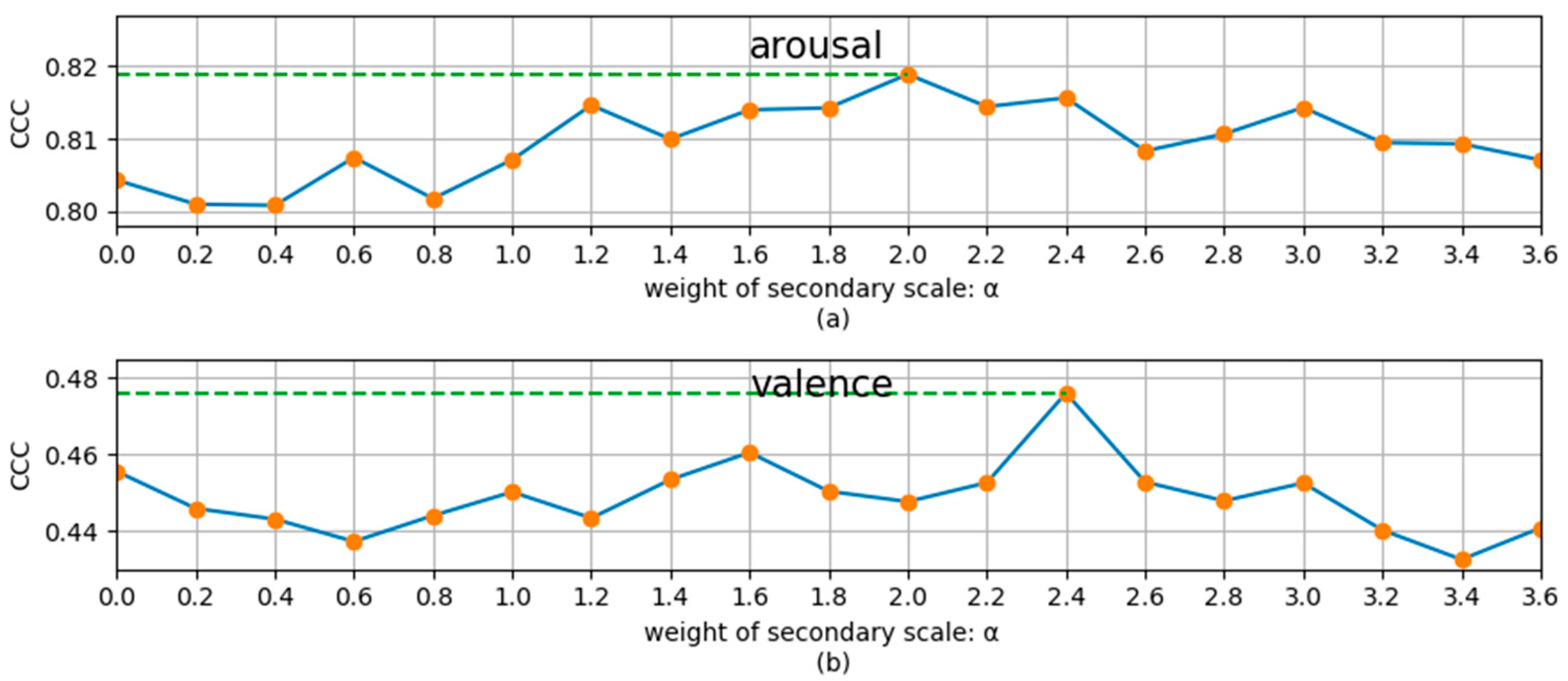
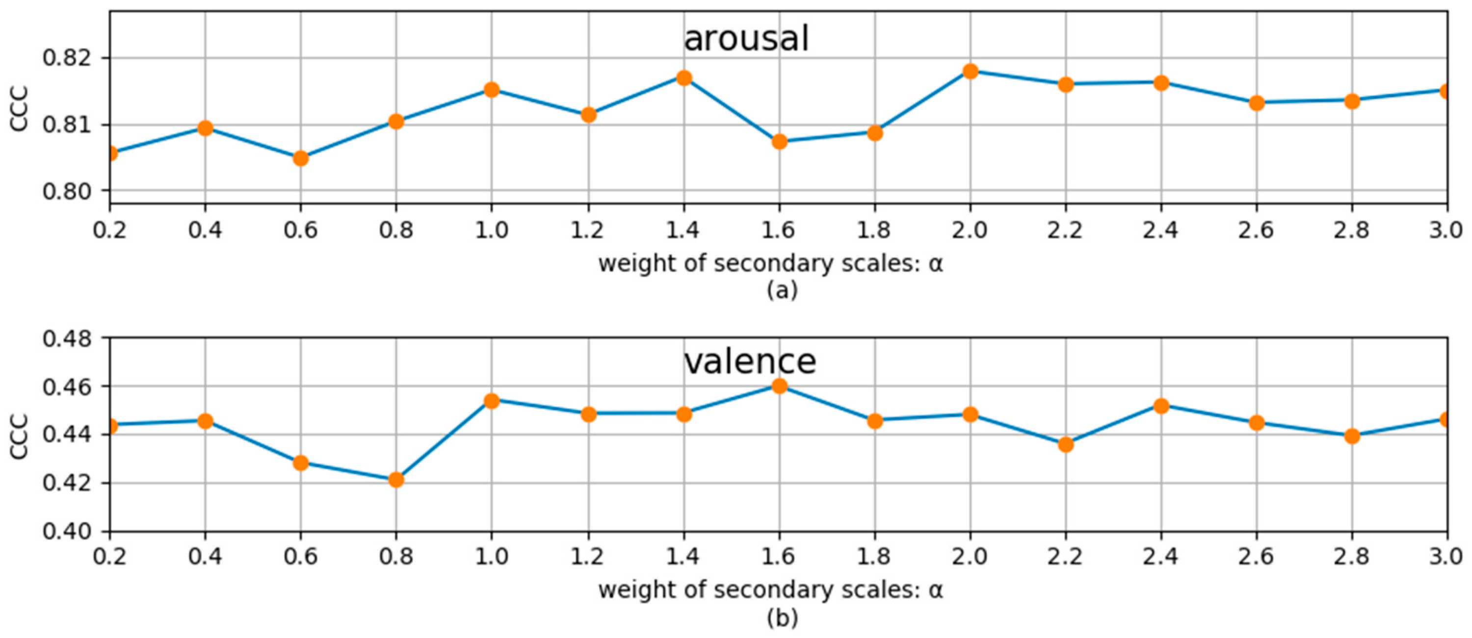
To study the influence of the weight coefficient $\alpha$ of the secondary scale, we used different $\alpha$ to perform the MSMT experiments. The experimental results for the development set for arousal and valence dimensions are shown in Figure 4, where $\alpha =0$ means that only the main scale was used. From Figure 4, we can see that, for the recognition of the two dimensions, the recognition performance slightly decreases when the secondary task is applied and then first increases and then decreases with the increase in $\alpha$. For the arousal and valence dimension, the best performance (the results in

Table 5. The MSMT recognition results on the development and test2 set after exchanging the main and secondary scales in Section 4.4.2.

Dimension	Development Set	Test2 Set
Arousal	0.779	0.671
Valence	0.425	0.465

) is achieved when $\alpha$ is about 2 and 2.4, respectively. This indicates that by choosing an appropriate weight coefficient, $\alpha$, the continuous dimension emotion recognition on the main scale can be promoted by the recognition on the secondary scale. Experiments show that the best performance is generally obtained when $\alpha \le 3$. Therefore, all our MSMT experiments chose the best alpha in the interval (0,3].

To study the influence of the choice of the main and secondary scales on the MSMT recognition results, we exchange the main and the secondary scale in Section 4.4.2. That is, for the arousal and valence dimensions, 110 (frames) and 130 (frames) are taken as the secondary scale, respectively, and 1 (frame) is taken as the main scale. The corresponding MSMT results are shown in Table 5. By comparing these with Table 1, it can be seen that there is no obvious difference between the MSMT results and SSST results with pooling size 1 for the two dimensions. This shows that the shortcomings of high noise and lack of contextual information in small-scale continuous dimensional emotion recognition are difficult to improve by large-scale dimensional emotion recognition training. Therefore, we chose the larger scales 110 (for arousal) and 130 (for valence) as the main scales in the Section 4.4.2 experiments.

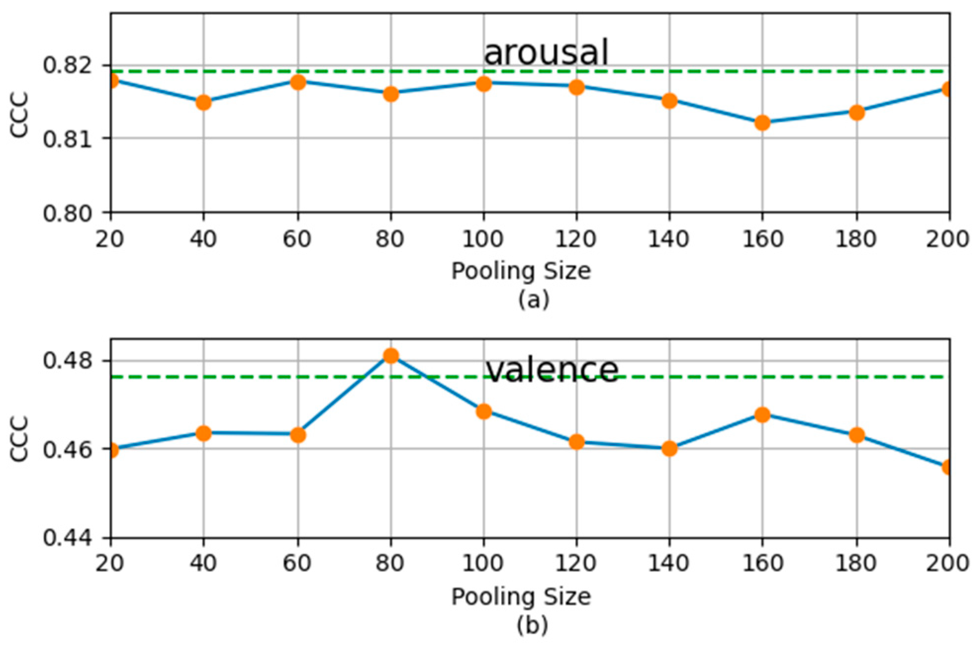
For the fixed main scale, to study the influence of different secondary scales on the recognition results, we took different scales from 1 to 200 (frames) as secondary scales for research. The corresponding MSMT recognition results are shown in Figure 5. From Figure 5, we can see that, for both dimensions, when the secondary scale is 1 (frame), the system achieves the best performance. As the secondary scales increase, the performance of the system decreases. This is consistent with our expectations. The small-scale features and labels are rich in detailed information. Although they lack contextual information and are rich in noise, they can significantly improve the main-scale performance of continuous dimensional emotion recognition when used as the secondary scale. With the increase in the secondary scale, less and less detailed information is provided, so main-scale recognition performance is helped less and less, and can even be hurt. Therefore, in Section 4.4.2, we chose 1 (frame) (2 frames for arousal dimension in the SEMAINE set) as the secondary scale for arousal and valence dimensions. We can also see from Figure 5 that when the secondary scale is larger than half of the main scale, MSMT results have no obvious advantage over the SSST results. Therefore, when we take the secondary scale, even if we do not take 1 (frame), no more than half of the main scale should be used.

To study the influence of the number of secondary scales on the MSMT recognition results, we fixed the best combination of the aforementioned main and secondary scales (i.e., the main scales are 110 and 130 (frames) for arousal and valence dimension, respectively, and the secondary scales are both 1 (frames)). Then, we took different scales from 20 to 200 (frames) as the second secondary scale. The two secondary scales share the same secondary weight coefficient. The corresponding MSMT recognition results are shown in Figure 6. From Figure 6, we can see that, when we add another secondary scale, there is no significant change in MSMT recognition performance, regardless of the added scale. Therefore, two scales are sufficient for continuous dimensional.

Further, we examined the relationship between recognition performance and the weight coefficient of secondary tasks in the case of three tasks. The experimental results are shown in Figure 7. Comparing Figure 7 with Figure 4, we find that, to obtain a good performance in the case with two tasks, we need to carefully select the weight coefficient. For the case of three tasks, although the optimal performance was not improved, the recognition performance was not as sensitive to the weight coefficient. For the arousal dimension, when $\alpha >1$, good results can be obtained for almost every weight coefficient. This will be convenient for practical application.

4.4.4. Comparison

Since the continuous dimension emotion recognition based on audio is a relatively challenging task, there are not many works in this area. Moreover, some are different from the dataset we use, some use different split methods for the dataset, and different researchers may use different audio features, which makes it difficult to compare the results. To make a fair comparison, we try to list the results obtained with the same dataset, the same train/development/test split method and the same or the similar audio features, and compare them with our results. For the RECOLA dataset, we did not find any results using the same test set as we used. We only compared the results for the development set. For the SEMAINE dataset, we did not find any work using the same features as ours, so we listed several better results and compared them. Since most of the results using the SEMAINE dataset were measured by the average PCC of each sequence, we present the average PCC results on the development and test sets. The results for the development subset of RECOLA dataset are shown in

Table 6. The recognition results (measure by ccc) on the development set of the RECOLA dataset.

Method	Development Set
	Arousal	Valence
MSMT (our model)	0.819	0.475
Valstar et al. [25]	0.796	0.455
Li et al. [10]	0.787	0.465
Chao et al. [15] *	0.798	0.483
Ringeval et al. [24] *	0.287	0.069

* The features used in the literature are similar to ours.

. The results for the development subset and the test subset of SEMAINE dataset are shown in

Table 7. The recognition results (measured by the average PCC of each sequence) on the development subset and the test subset of the SEMAINE dataset.

Model	Development Set		Test Set
	Arousal	Valence	Arousal	Valence
MSMT (our model)	0.389	0.171	0.326	0.085
Savran et al. [33]	0.215	0.297	0.74	0.149
Nicolle et al. [34] **	0.509	0.017	-	-
Pei et al. [35] **	0.398	0.143	-	-

** In the literature, several methods were used to obtain multiple audio-based dimensional prediction results, and we chose the best one. The results of the test set are not given.

.

Table 6 shows that our method can achieve better results on the RECOLA set when using the same or similar features. From Table 7, we can see that our method can offer competitive results in the case of different features.

5. Conclusions

In this paper, a novel MSMT model was presented to utilize features and dimensional emotion labels on different timescales. We built this model based on a DBN with only one hidden layer. All the features share the same hidden parameters, followed by different temporal pooling layers, but have the same linear layer parameters. The combination of the MSEs of different tasks is used as the objective function. The system is initialized by unsupervised pre-training, then fine-tuned by the MSMT learning.

To illustrate the effectiveness of our model, we conducted extensive experiments on RECOLA and SEMAINE datasets. We found that, even if we add a secondary scale to the single scale with the best performance, its performance can still be improved. Of course, this increase is closely related to the selection of the secondary scale and the weight coefficient of the secondary scale, which needs to be carefully selected in practical operation. If we add the third scale, based on the combination of main and secondary scales with the best performance, it will not significantly improve the optimal performance. However, the result is not very sensitive to the weight coefficient. Therefore, this combination of three tasks is an infallible choice when there are no conditions for parameter optimization. Through the experimental results for the two datasets, this model is shown to have no definite law for which the dimensions of arousal and value have a better performance improvement effect. On the RECOLA set, the performance improvement for the arousal dimension is significantly better than that of the valence dimension. On the SEMAINE set, the result is the opposite. This may be caused by different data characteristics, due to the different annotation methods of the dataset. As can be seen from Figure 3, for the results of the arousal dimension, when the pooling size is greater than 560, the degradation of recognition performance is not obvious. There may even be an increase. This shows that the noise reduction caused by using a larger scale is much greater than the loss of information reduction. This may be due to the large noise caused by the fact that the annotator needs to label the values of several dimensions at the same time during the rating process.

In our work, we only used the extended Geneva Minimalistic Acoustic Parameter Set as our feature, and whether this will have better effects on other feature types remains to be further studied. Our experiments were only carried out on the audio modality. Whether it is effective on other modalities (such as video, physiologic modality, etc.) is also an issue for further study.