
Industrial Internet of Things for Condition Monitoring and Diagnosis of Dry Vacuum Pumps in Atomic Layer Deposition Equipment


Abstract
:1. Introduction
2. Subject Matter
2.1. Equipment Degradation Mechanism
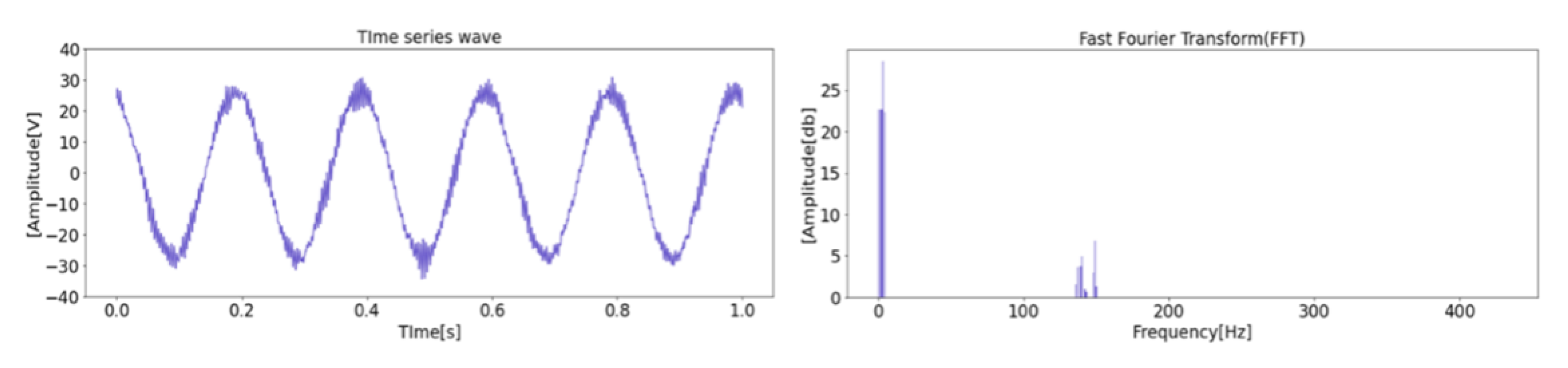
2.2. Mechanical Vibration Analysis
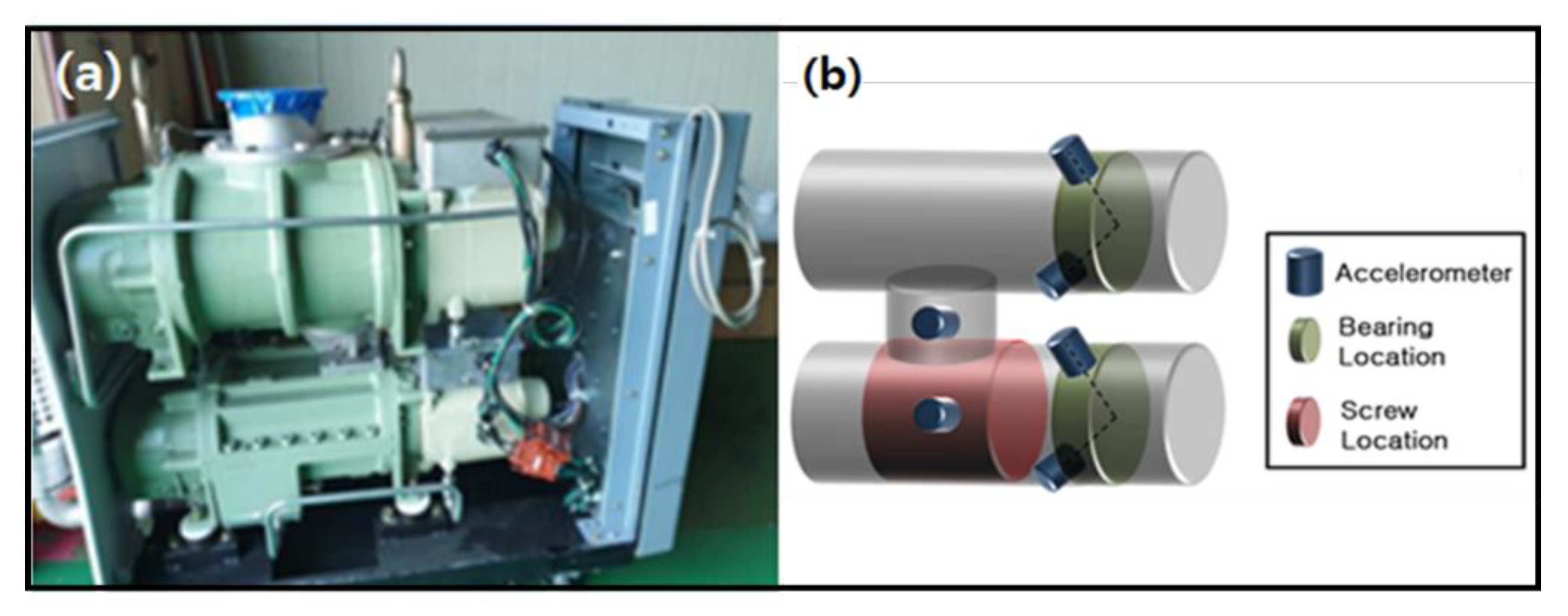
3. In Situ Vibration Data Acquisition
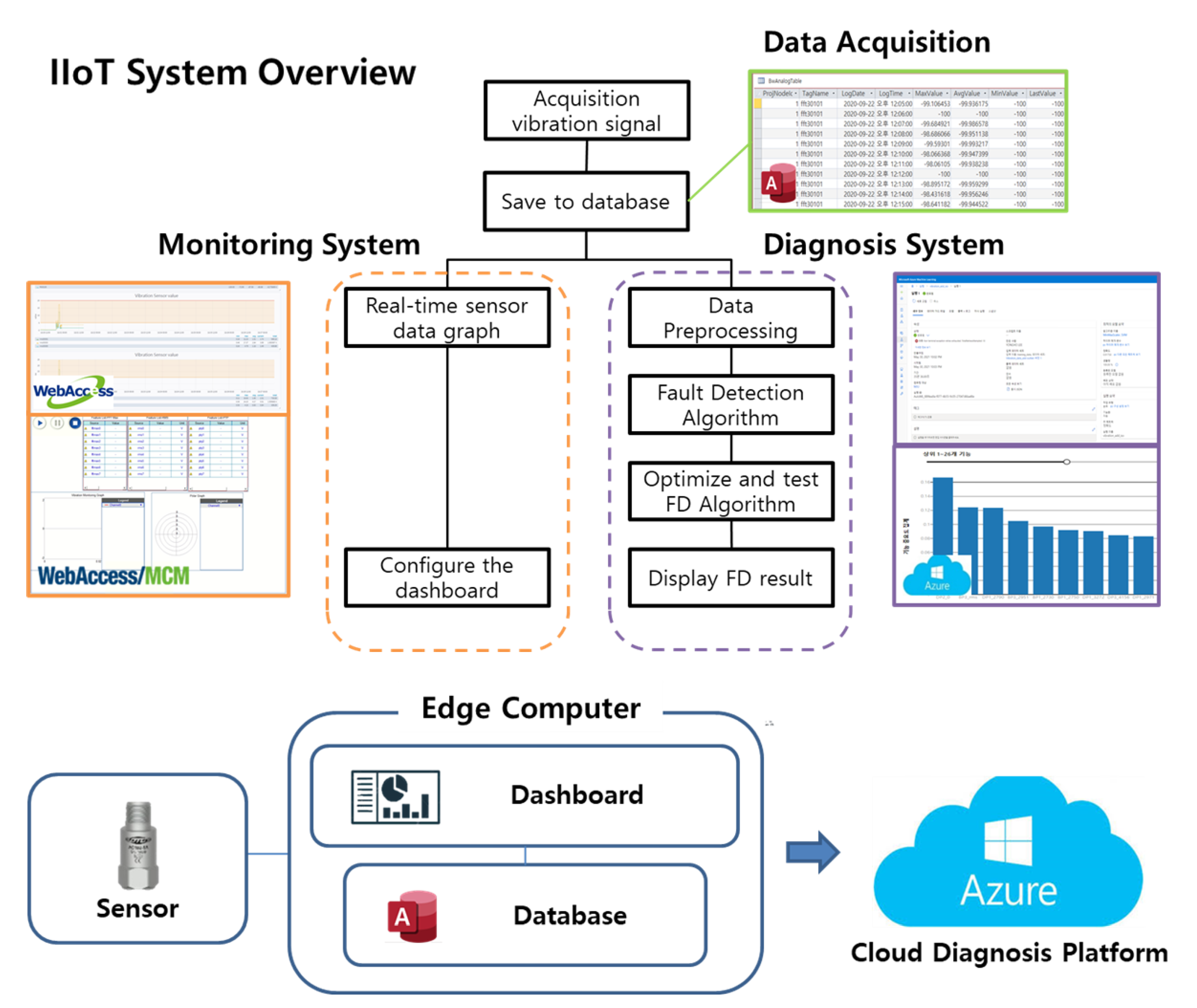
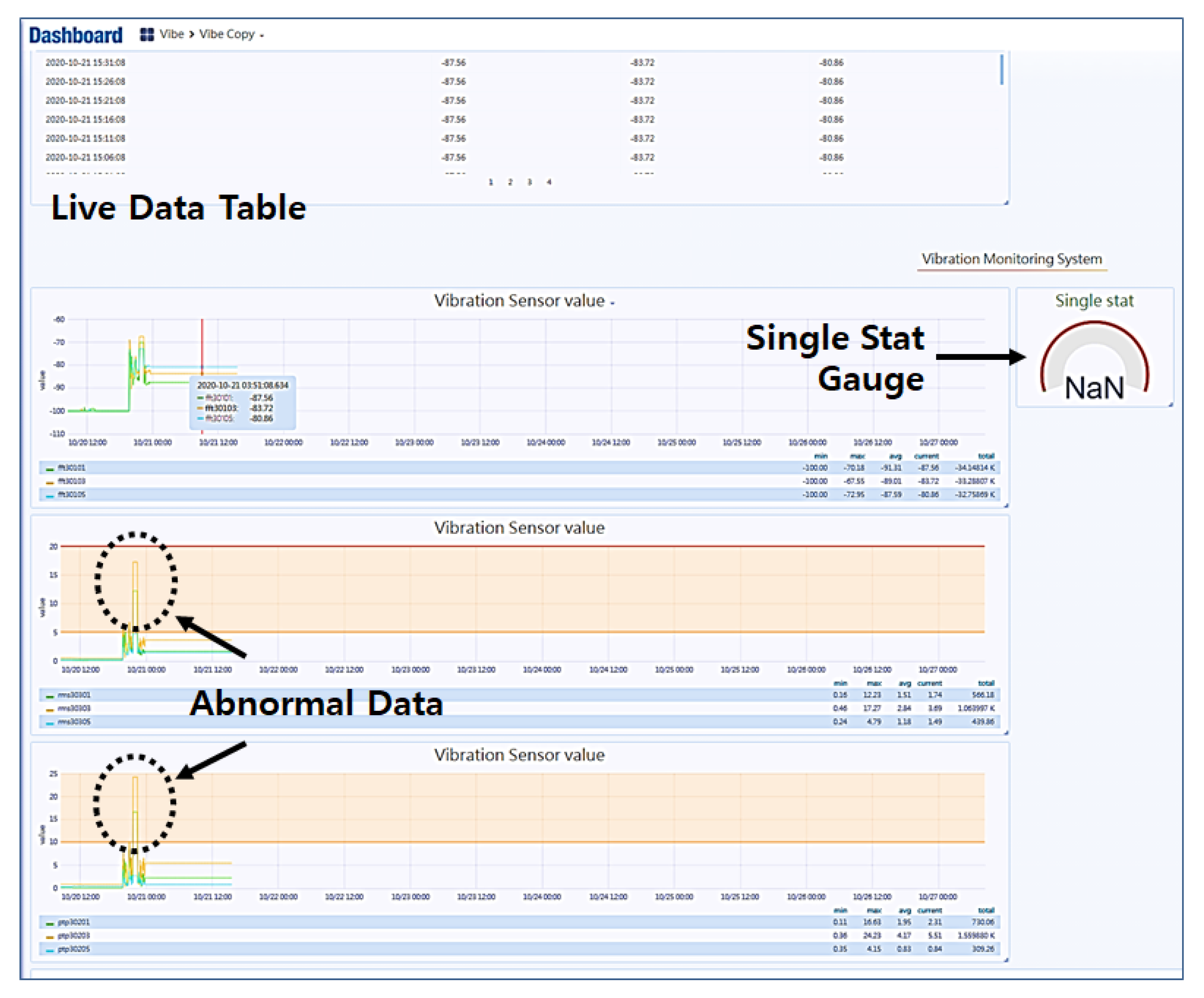
4. Monitoring and Diagnostic System
5. Conclusions
Author Contributions
Funding
Acknowledgments
Conflicts of Interest
Appendix A
| Algorithm A1 SVM Pseudo-Code | |
| 1: | Input: parameters: |
| 2: | out = array of SVM outputs |
| 3: | target = array of booleans: is ith example a positive example? |
| 4: | prior1 = number of positive examples |
| 5: | prior0 = number of negative examples |
| 6: | Output: Parameters of sigmoid |
| 7: | A = 0 |
| 8: | B = log((𝑝𝑟𝑖𝑜𝑟0 + 1)/(𝑝𝑟𝑖𝑜𝑟1 + 1)) |
| 9: | log((prior0 + 1)/(prior1 + 1)) |
| 10: | hiTarget = (prior1 + 1)/(prior1 + 2) |
| 11: | loTarget = 1/(prior0 + 2) |
| 12: | lambda = 1e−3 |
| 13: | olderr = 1e300 |
| 14: | pp = temp array to store current estimate of probability of examples |
| 15: | set all pp array elements to (prior1 + 1)/(prior0 + prior1 + 2) |
| 16: | count = 0 |
| 17: | for it = 1 to 100 |
| 18: | a = 0, b = 0, c = 0, d = 0, e = 0 |
| 19: | //First, compute Hessian & gradient of error function |
| 20: | //with respect ro A & B |
| 21: | for i = 1 to len { |
| 22: | if (target[i]) |
| 23: | t = hiTarget |
| 24: | Else |
| 25: | t = loTarget |
| 26: | d1 = 𝑝𝑝[𝑖] − 𝑡 |
| 27: | d2 = 𝑝𝑝[𝑖]∗(1 − 𝑝𝑝[𝑖]) |
| 28: | a + = 𝑜𝑢𝑡[𝑖]∗𝑜𝑢𝑡[𝑖]∗𝑑2 |
| 29: | b + = 𝑑2 |
| 30: | c + = 𝑜𝑢𝑡[𝑖]∗𝑑2 |
| 31: | d + = 𝑜𝑢𝑡[𝑖]∗𝑑1 |
| 32: | e + = 𝑑1 |
| 33: | //If gradient is really tiny, then stop |
| 34: | if (𝑎𝑏𝑠(𝑑) < 1𝑒−9 && 𝑎𝑏𝑠(𝑒) < 1𝑒−9) |
| 35: | Break |
| 36: | oldA = A |
| 37: | oldB = B |
| 38: | err = 0 |
| 39: | //Loop until goodness of fit increases |
| 40: | while (1) { |
| 41: | det = (𝑎 + 𝑙𝑎𝑚𝑏𝑑𝑎)∗(𝑏 + 𝑙𝑎𝑚𝑏𝑑𝑎) − 𝑐∗𝑐 |
| 42: | if (det == 0) {//if determinant of Hessian is zero, |
| 43: | //increase stabilizer |
| 44: | 𝑙𝑎𝑚𝑏𝑑𝑎∗ = 10 |
| 45: | Continue |
| 46: | } |
| 47: | A = 𝑜𝑙𝑑𝐴 + ((𝑏+𝑙𝑎𝑚𝑏𝑑𝑎)∗𝑑 − 𝑐∗𝑒)/𝑑𝑒t |
| 48: | B = 𝑜𝑙𝑑𝐵 + ((𝑎 + 𝑙𝑎𝑚𝑏𝑑𝑎)∗𝑒 − 𝑐∗𝑑)/𝑑𝑒𝑡 |
| 49: | //Now, compute the goodness of fit |
| 51: | for i = 1 to len { |
| 52: | p = 1/(1 + exp(𝑜𝑢𝑡[𝑖]∗𝐴 + 𝐵 )) |
| 53: | pp[i] = p |
| 54: | //At this step, make sure log(0) returns -200 |
| 55: | 𝑒𝑟𝑟 − = 𝑡∗log(𝑝) + (1 − 𝑡)∗log(1 − 𝑝) |
| 56: | } |
| 57: | if (𝑒𝑟𝑟 < 𝑜𝑙𝑑𝑒𝑟𝑟∗(1 + 1𝑒 − 7)) { |
| 58: | 𝑙𝑎𝑚𝑏𝑑𝑎∗ = 0.1 |
| 59: | Break |
| 60: | } |
| 61: | //error did not decrease: increase stabilizer by factor of 10 |
| 62: | //& try again |
| 63: | 𝑙𝑎𝑚𝑏𝑑𝑎∗ = 10 |
| 64: | if (𝑙𝑎𝑚𝑏𝑑𝑎 ≥ 1𝑒6)//something is broken, Give up |
| 65: | Break |
| 66: | } |
| 67: | diff = err-older |
| 68: | scale = 0.5∗(𝑒𝑟𝑟 + 𝑜𝑙𝑑𝑒𝑟𝑟 + 1) |
| 69: | if (𝑑𝑖𝑓𝑓 > − 1𝑒 − 3∗ 𝑠𝑐𝑎𝑙𝑒&&𝑑𝑖𝑓𝑓 < 1𝑒 − 7∗𝑠𝑐𝑎𝑙𝑒) |
| 70: | count ++ |
| 71: | Else |
| 72: | count = 0 |
| 73: | older = err |
| 74: | if (count == 3) |
| 75: | Break |
| 76: | } |
| Algorithm A2 Stacked Ensemble Classifier Pseudo-Code | |
| 1: | Input: Dataset 𝐷 = {(𝑥1,𝑦1),(𝑥2,𝑦2),⋯,(𝑥𝑚,𝑦𝑚)}; |
| 2: | Base-classifier 𝑓1 = 𝑅𝐹1, 𝑓2 = 𝑅𝐹2, 𝑓3 = 𝐸𝑇1, 𝑓4 = 𝐸𝑇2 |
| 3: | For 𝑡 = 1,⋯,4; |
| 4: | Train the base-classifiers in the first stage |
| 5: | ℎ𝑡 = 𝑓𝑡(𝐷); |
| 6: | End |
| 7: | For i = 1,2,⋯,𝑚: |
| 8: | for 𝑡 = 1,⋯,4: |
| 9: | Generate new feature vector for each sample |
| 10: | 𝑧𝑖𝑡 = ℎ𝑡(𝑥𝑖); |
| 11: | End |
| 12: | 𝐷′ = 𝐷′∪((𝑧𝑖1,⋯,zi4),yi); |
| 13: | End |
| 14: | Train the meta-classifier in the second stage |
| 15: | ℎ′ = 𝑓(𝐷′); |
| 16: | Output: 𝐻(𝑥) = ℎ′(ℎ1(𝑥),…,ℎ4(𝑥)) |
| Algorithm A3 LightGBM Pseudo-Code | |
| 1: | Input: 𝐼: training data, 𝑑: max depth |
| 2: | Input: 𝑚: feature dimension |
| 3: | nodeSet←{0}.ree nodes in current level |
| 4: | rowSet ← {{0, 1, 2,…}} ▷ data indices in tree nodes |
| 5: | for 𝑖 = 1 to𝑑do |
| 6: | for 𝑛𝑜𝑑𝑒 in 𝑛𝑜𝑑𝑒𝑆𝑒𝑡 do |
| 7: | usedRows ←𝑟𝑜𝑤𝑆𝑒𝑡[𝑛𝑜𝑑𝑒] |
| 8: | for𝑘 = 1 to𝑚do |
| 9: | H ← new Histogram() |
| 10: | ▷ Build histogram |
| 11: | for𝑗in𝑢𝑠𝑒𝑑𝑅𝑜𝑤𝑠do |
| 12: | bin ← I.f[k][j].bin |
| 13: | H [bin].y H [bin].y + I.y[j] |
| 14: | H [bin].n H [bin].n + 1 |
| 15: | Find the best split on histogram H. |
| 16: | … |
| 17: | Update 𝑟𝑜𝑤𝑆𝑒𝑡 and 𝑛𝑜𝑑𝑒𝑆𝑒𝑡 according to the best split points. |
| 18: | … |
| 19: | Input: 𝐼: training data, 𝑑: iterations |
| 20: | Input: 𝑎: sampling ratio of large gradient data |
| 21: | Input: 𝑏: sampling ratio of small gradient data |
| 22: | Input: 𝑙𝑜𝑠𝑠: loss function, 𝐿: weak learner |
| 23: | models ← { }, fact ← (1−𝑎)/𝑏 |
| 24: | topN ←𝑎 × len(𝐼),randN← b ×len(I) |
| 25: | for 𝑖 = 1 to𝑑do |
| 26: | preds ← models.predict(I) |
| 27: | g ←𝑙𝑜𝑠𝑠(I, preds), w ← {1,1,…} |
| 28: | sorted ← GetSortedIndices(abs(g)) |
| 29: | topSet ← sorted [1:topN] |
| 30: | randSet ← RandomPick(sorted[topN:len(I)], randN) |
| 31: | usedSet ← topSet + randSet |
| 32: | w[randSet] × = fact ▷ Assign weight 𝑓𝑎𝑐𝑡 to the small gradient data. |
| 33: | newModel ← L(I [usedSet],− g[usedSet], w[usedSet]) |
| 34: | models.append(newModel) |
| Algorithm A4 XGboost Pseudo-Code | |
| 1: | Input: I, instance set of current node |
| 2: | Input: d, feature dimension |
| 3: | 𝑔𝑎𝑖𝑛← 0 |
| 4: | |
| 5: | for 𝑞 = 1 to 𝑄 do: |
| 6: | 𝐺L←0,𝐻𝐿←0 |
| 7: | for 𝑗𝑖𝑛𝑠𝑜𝑟𝑡𝑒𝑑 (I, 𝑏𝑦𝑥jq) do |
| 8: | 𝐺𝐿← 𝐺𝐿 + 𝑔𝑗, 𝐻𝐿← 𝐻𝐿 + h𝑗 |
| 9: | 𝐺𝑅←𝐺−𝐺𝐿, 𝐻𝑅←𝐻 − 𝐻𝐿 |
| 10: | |
| 11: | End for |
| 12: | End for |
| 13: | Output: Split with max score |
| Algorithm A5 Random Forest Pseudo-Code | |
| 1: | Require: 𝐼𝐷𝑇(a decision tree inducer), |
| 2: | (the training set), |
| 3: | (the subsample size), 𝑁 (number of attributes used in each node) |
| 4: | Ensure: 𝑀𝑡;𝑡 = 1, …,𝑇 |
| 5: | 𝑡← 2 |
| 6: | Repeat |
| 7: | 𝑆𝑡← Sample 𝜇 instances from 𝑆 with replacement |
| 8: | Build classifier 𝑀𝑡 using 𝐼𝐷𝑇(𝑁) on 𝑆𝑡 |
| 9: | 𝑡 ++ |
| 10: | until 𝑡 > 𝑇 |
| Algorithm A6 Extra-Trees Splitting Algorithm Pseudo-Code | |
| 1: | Split_a_node(𝑆) |
| 2: | Input: the local learning subset S corresponding to the node we want to split |
| 3: | ] or nothing |
| 4: | If Stop_split(S) is TRUE then return nothing |
| 5: | |
| 6: | among all non constant (in S) candidate attributes; |
| 7: | , ∀i = 1, … K; |
| 8: | Return a split s∗ such that Score(s∗, S) = maxi=1,…,K Score(si, S). |
| 9: | |
| 10: | Pick_a_random_split(S,a) |
| 11: | Inputs: a subset S and an attribute a |
| 12: | Output: a split |
| 13: | denote the maximal and minimal value of a in S; |
| 13: | denote the maximal and minimal value of a in S; |
| 14: | ]; |
| 15: | . |
| 16: | |
| 17: | Stop_split(S) |
| 18: | Input: a subset S |
| 19: | Output: a Boolean |
| 20: | If |S | < nmin, then return TRUE; |
| 21: | If all attributes are constant in S, then return TRUE; |
| 22: | If the output is constant in S, then return TRUE; |
| 23: | Otherwise, return FALSE. |
References
- Antao, L.; Pinto, R.; Reis, J.; Goncalves, G. Requirements for Testing and Validating the Industrial Internet of Things. In Proceedings of the 2018 IEEE International Conference on Software Testing, Verification and Validation Workshops (ICSTW), Västerås, Sweden, 9–13 April 2018; pp. 110–115. [Google Scholar] [CrossRef]
- Serpanos, D.; Wolf, M. Internet-of-Things (IoT) Systems; Springer: Berlin/Heidelberg, Germany, 2018; pp. 37–54. [Google Scholar] [CrossRef]
- Chen, Y.; Lee, G.M.; Shu, L.; Crespi, N. Industrial Internet of Things-Based Collaborative Sensing Intelligence: Framework and Research Challenges. Sensors 2016, 16, 215. [Google Scholar] [CrossRef] [PubMed]
- Sisinni, E.; Saifullah, A.; Han, S.; Jennehag, U.; Gidlund, M. Industrial Internet of Things: Challenges, Opportunities, and Directions. IEEE Trans. Ind. Inform. 2018, 14, 4724–4734. [Google Scholar] [CrossRef]
- Civerchia, F.; Bocchino, S.; Salvadori, C.; Rossi, E.; Maggiani, L.; Petracca, M. Industrial Internet of Things monitoring solution for advanced predictive maintenance applications. J. Ind. Inf. Integr. 2017, 7, 4–12. [Google Scholar] [CrossRef]
- Razmi-Farooji, A.; Kropsu-Vehkaperä, H.; Härkönen, J.; Haapasalo, H. Advantages and potential challenges of data management in e-maintenance. J. Qual. Maint. Eng. 2019, 25, 378–396. [Google Scholar] [CrossRef]
- Lade, P.; Ghosh, R.; Srinivasan, S. Manufacturing Analytics and Industrial Internet of Things. IEEE Intell. Syst. 2017, 32, 74–79. [Google Scholar] [CrossRef]
- Hong, S.J.; Lim, W.Y.; Cheong, T.; May, G.S. Fault Detection and Classification in Plasma Etch Equipment for Semiconductor Manufacturing e-Diagnostics. IEEE Trans. Semicond. Manuf. 2011, 25, 83–93. [Google Scholar] [CrossRef]
- Boyes, H.; Hallaq, B.; Cunningham, J.; Watson, T. The industrial internet of things (IIoT): An analysis framework. Comput. Ind. 2018, 101, 1–12. [Google Scholar] [CrossRef]
- Suh, Y.J.; Choi, J.Y. Efficient Fab facility layout with spine structure using genetic algorithm under various material-handling considerations. Int. J. Prod. Res. 2021, 1–14. [Google Scholar] [CrossRef]
- Kumar, A.; Bhattacharjee, N.; Patel, B.; Laloë, J.-B.; Famodu, O.O.; Ferain, L. Stratege for Reducing Particle Defects in Ti and TiN Thin-Film Deposition Process. IEEE Trans. Semi. Manufac. 2018, 32, 48–53. [Google Scholar] [CrossRef]
- Jones, C.P. Thin Film Processes: Abatement of Waste Gases from Plasma Assisted Material Processes. In Proceedings of the 2020 China Semiconductor Technology International Conference (CSTIC), Shanghai, China, 26 June–17 July 2020; pp. 1–3. [Google Scholar] [CrossRef]
- Lessard, P.A. Dry vacuum pumps for semiconductor processes: Guidelines for primary pump selection. J. Vac. Sci. Technol. A 2000, 18, 1777–1781. [Google Scholar] [CrossRef]
- Zhan, H.; Li, N.; Wang, Y.; Wang, X.; Lin, S. Fault Diagnosis Method for Vacuum Pump of Space Environment Simulator. In Proceedings of the 2016 IEEE 11th Conference on Industrial Electronics and Applications (ICIEA), Hefei, China, 5–7 June 2016; pp. 1703–1707. [Google Scholar] [CrossRef]
- Ainapure, A.; Li, X.; Singh, J.; Yang, Q.; Lee, J. Deep Learning-Based Cross-Machine Health Identification Method for Vacuum Pumps with Domain Adaptation. Procedia Manuf. 2020, 48, 1088–1093. [Google Scholar] [CrossRef]
- Rui, X.; Liu, J.; Li, Y.; Qi, L.; Li, G. Research on fault diagnosis and state assessment of vacuum pump based on acoustic emission sensors. Rev. Sci. Instrum. 2020, 91, 025107. [Google Scholar] [CrossRef]
- LaRose, J.; Barker, J.; Finlay, B.; Trinidad, A.; Guyer, C.; Weinstein, J.; Conerney, B.; Ray, D.; Perry, J.; Tarnawskyj, W.; et al. Predictive Maintenance of Pump and Abatement Equipment in a 300mm Semiconductor Fab. In Proceedings of the 2021 32nd Annual SEMI Advanced Semiconductor Manufacturing Conference (ASMC), Milpitas, CA, USA, 10–12 May 2021; pp. 1–4. [Google Scholar] [CrossRef]
- Jiang, W.; Spurgeon, S.K.; Twiddle, J.A.; Schlindwein, F.S.; Feng, Y.; Thanagasundram, S. A wavelet cluster-based band-pass filtering and envelope demodulation approach with application to fault diagnosis in a dry vacuum pump. Proc. Inst. Mech. Eng. Part C J. Mech. Eng. Sci. 2007, 221, 1279–1286. [Google Scholar] [CrossRef] [Green Version]
- Twiddle, J.A.; Jones, N.B.; Spurgeon, S.K. Fuzzy model-based condition monitoring of a dry vacuum pump via time and frequency analysis of the exhaust pressure signal. Proc. Inst. Mech. Eng. Part C J. Mech. Eng. Sci. 2008, 222, 287–293. [Google Scholar] [CrossRef]
- Butler, S.W.; Ringwood, J.V.; MacGearailt, N. Prediction of Vacuum Pump Degradation in Semiconductor Processing. IFAC Proc. Vol. 2009, 42, 1635–1640. [Google Scholar] [CrossRef] [Green Version]
- Hsieh, F.-C.; Chou, S.-C.; Lin, P.-H.; Chang, S.-W.; Chen, F.-Z.; Liao, T.-S.; Liu, D.-R.; Chiang, D. Monitoring on dry vacuum pump characteristics by mobile device. In Proceedings of the 2012 IEEE International Instrumentation and Measurement Technology Conference Proceedings, Graz, Austria, 13–16 May 2012; pp. 2444–2447. [Google Scholar] [CrossRef]
- Qiu, G.Q.; Gu, Y.K.; Chen, J.J. Selective health indicator for bearings ensemble remaining useful life prediction with genetic algorithm and Weibull proportional hazards model. Measurement 2020, 150, 107097. [Google Scholar] [CrossRef]
- Lee, K.; Song, D.; Lee, J.; Lee, C.-G.; Shin, G.-A.; Jung, S. Evaluating effectiveness of dust by-product treatment with scrubbers to mitigate explosion risk in ZrO2 atomic layer deposition process. J. Hazard. Mater. 2020, 400, 123284. [Google Scholar] [CrossRef]
- Bhatti, M.A.; Riaz, R.; Rizvi, S.S.; Shokat, S.; Riaz, F.; Kwon, S.J. Outlier detection in indoor localization and Internet of Things (IoT) using machine learning. J. Commun. Netw. 2020, 22, 236–243. [Google Scholar] [CrossRef]
- Kim, D.H.; Choi, J.E.; Ha, T.M.; Hong, S.J. Modeling with Thin Film Thickness using Machine Learning. J. Semicond. Disp. Technol. 2019, 18, 48–52. Available online: https://www.koreascience.or.kr/article/JAKO201919761177833.page (accessed on 6 October 2021).
- Puggini, L.; McLoone, S. An enhanced variable selection and Isolation Forest based methodology for anomaly detection with OES data. Eng. Appl. Artif. Intell. 2018, 67, 126–135. [Google Scholar] [CrossRef] [Green Version]
- Shukla, S.; Meghana, K.M.; Manjunatrh, C.R.; Santosh, N. Comparison of Wireless Network over Wired Network and its Type. Int. J. Res. -Granthaalayah 2017, 5, 14–20. [Google Scholar] [CrossRef]
- Bailey, C.; Hutchison, K.; Wilders, M. Vacuum Systems for ALD. Solid State Technol. 2006, 49, 30–33. [Google Scholar]
- Hur, M.; Lee, J.; Yoo, H.; Kang, W.; Song, Y.; Kim, D.; Lee, S. Reduction of byproduct particle size using low-pressure plasmas generated by a cylindrical-shaped electrode. Vacuum 2012, 86, 1834–1839. [Google Scholar] [CrossRef]
- ISO 18436-2: 2014 Condition Monitoring and Diagnostics of Machines—Requirements for Qualification and Assessment of Personnel—Part 2: Vibration Condition Monitoring and Diagnostics. Available online: https://www.iso.org/standard/50447.html (accessed on 6 October 2021).
- Liu, F.T.; Ting, K.M.; Zhou, Z.-H. Isolation Forest. In Proceedings of the 2008 Eighth IEEE International Conference on Data Mining, Pisa, Italy, 15–19 December 2008; pp. 413–422. [Google Scholar] [CrossRef]
- Vishwakarma, M.; Purohit, R.; Harshlata, V.; Rajput, P. Vibration Analysis & Condition Monitoring for Rotating Machines: A Review. Mater. Today Proc. 2017, 4, 2659–2664. [Google Scholar] [CrossRef]
- John, C.P. Probabilistic Outputs for Support Vector Machines and Comparisons to Regularized Likelihood Methods. Adv. Large Margin Classif. 1999, 10, 61–74. Available online: https://citeseerx.ist.psu.edu/viewdoc/versions?doi=10.1.1.41.1639 (accessed on 6 October 2021).
- Chen, C.; Zhang, Q.; Yu, B.; Yu, Z.; Skillman-Lawrence, P.; Ma, Q.; Zhang, Y. Improving protein-protein interactions prediction accuracy using XGBoost feature selection and stacked ensemble classifier. Comput. Biol. Med. 2020, 123, 103899. [Google Scholar] [CrossRef] [PubMed]
- Ke, G.; Meng, Q.; Finley, T.; Wang, T.; Chen, W.; Ma, W.; Ye, Q.; Liu, T.-Y. LightGBM: A Highly Efficient Gradient Boosting Decision Tree. Adv. Neural Inf. Processing Syst. 2017, 30, 3146–3154. Available online: https://proceedings.neurips.cc/paper/2017/hash/6449f44a102fde848669bdd9eb6b76fa-Abstract.html (accessed on 6 October 2021).
- Zhang, W.; Zhao, X.; Li, Z. A Comprehensive Study of Smartphone-Based Indoor Activity Recognition via Xgboost. IEEE Access 2019, 7, 80027–80042. [Google Scholar] [CrossRef]
- Lior, R. Ensemble-Based Classifiers. Artif. Intell. Rev. 2010, 33, 1–39. [Google Scholar] [CrossRef]
- Geurts, P.; Ernst, D.; Wehenkel, L. Extremely randomized trees. Mach. Learn. 2006, 63, 3–42. [Google Scholar] [CrossRef] [Green Version]


| Experiment Condition | Accuracy | Balanced Accuracy | F1_Score | Recall Score Micro | Log_Loss |
|---|---|---|---|---|---|
| MinMaxScaler, SVM | 0.918 | 0.672 | 0.918 | 0.918 | 0.217 |
| StackEnsemble | 0.916 | 0.661 | 0.916 | 0.916 | 0.222 |
| RobustScaler, SVM | 0.909 | 0.609 | 0.909 | 0.909 | 0.235 |
| MaxAbsScaler, LightGBM | 0.907 | 0.552 | 0.907 | 0.907 | 0.250 |
| StandardScalerWrapper, LightGBM | 0.908 | 0.563 | 0.908 | 0.908 | 0.248 |
| SparseNormalizer, XGBoostClassifier | 0.906 | 0.570 | 0.906 | 0.906 | 0.354 |
| Experiment Condition | Accuracy | Balanced Accuracy | F1_Score | Recall Score Micro | Log_Loss |
|---|---|---|---|---|---|
| MinMaxScaler, RandomForest | 1.000 | 1.000 | 1.000 | 1.000 | 0.0000005 |
| StandardScalerWrapper, RandomForest | 1.000 | 1.000 | 1.000 | 1.000 | 0.00001 |
| SparseNormalizer, XGBoostClassifier | 1.000 | 1.000 | 1.000 | 1.000 | 0.00004 |
| MaxAbsScaler, XGBoostClassifier | 1.000 | 1.000 | 1.000 | 1.000 | 0.00005 |
| MaxAbsScaler, LightGBM | 1.000 | 1.000 | 1.000 | 1.000 | 0.0003 |
| StandardScalerWrapper, ExtremeRandomTrees | 1.000 | 1.000 | 1.000 | 1.000 | 0.001 |
Publisher’s Note: MDPI stays neutral with regard to jurisdictional claims in published maps and institutional affiliations. |
© 2022 by the authors. Licensee MDPI, Basel, Switzerland. This article is an open access article distributed under the terms and conditions of the Creative Commons Attribution (CC BY) license (https://creativecommons.org/licenses/by/4.0/).
Share and Cite
Lee, Y.; Kim, C.; Hong, S.J. Industrial Internet of Things for Condition Monitoring and Diagnosis of Dry Vacuum Pumps in Atomic Layer Deposition Equipment. Electronics 2022, 11, 375. https://doi.org/10.3390/electronics11030375
Lee Y, Kim C, Hong SJ. Industrial Internet of Things for Condition Monitoring and Diagnosis of Dry Vacuum Pumps in Atomic Layer Deposition Equipment. Electronics. 2022; 11(3):375. https://doi.org/10.3390/electronics11030375
Chicago/Turabian StyleLee, Yongho, Chanyoung Kim, and Sang Jeen Hong. 2022. "Industrial Internet of Things for Condition Monitoring and Diagnosis of Dry Vacuum Pumps in Atomic Layer Deposition Equipment" Electronics 11, no. 3: 375. https://doi.org/10.3390/electronics11030375
APA StyleLee, Y., Kim, C., & Hong, S. J. (2022). Industrial Internet of Things for Condition Monitoring and Diagnosis of Dry Vacuum Pumps in Atomic Layer Deposition Equipment. Electronics, 11(3), 375. https://doi.org/10.3390/electronics11030375