Article

Synthetic Energy Data Generation Using Time Variant Generative Adversarial Network

Centre for Cyber Security Research and Innovation (CSRI), School of IT, Deakin University, Geelong, VIC 3216, Australia
*
Author to whom correspondence should be addressed.
Electronics 2022, 11(3), 355; https://doi.org/10.3390/electronics11030355
Submission received: 2 December 2021 / Revised: 10 January 2022 / Accepted: 19 January 2022 / Published: 24 January 2022
(This article belongs to the Special Issue 10th Anniversary of Electronics: Advances in Networks)

Abstract

:
Energy consumption data is being used for improving the energy efficiency and minimizing the cost. However, obtaining energy consumption data has two major challenges: (i) data collection is very expensive, time-consuming, and (ii) security and privacy concern of the users which can be revealed from the actual data. In this research, we have addressed these challenges by using generative adversarial networks for generating energy consumption profile. We have successfully generated synthetic data which is similar to the real energy consumption data. On the basis of the recent research conducted on TimeGAN, we have implemented a framework for synthetic energy consumption data generation that could be useful in research, data analysis and create business solutions. The framework is implemented using the real-world energy dataset, consisting of energy consumption data of the year 2020 for the Australian states of Victoria, New South Wales, South Australia, Queensland and Tasmania. The results of implementation is evaluated using various performance measures and the results are showcased using visualizations along with Principal Component Analysis (PCA) and t-distributed stochastic neighbor embedding (TSNE) plots. Overall, experimental results show that Synthetic data generated using the proposed implementation possess very similar characteristics to the real dataset with high comparison accuracy.

1. Introduction

Today’s modernized energy system or simply ‘Smart Grid’ is the result of advanced sensing, automation and control. Moreover, introduction of distributed renewable energy resources have brought the generation close to the consumer and introduce the concept of bi-directional power flows. For effective monitoring and control of the smart grid systems, sensors and measurement devices have been incorporated throughout the network [1]. At low voltage customer level, it was not well monitored until the recent years when the use of smart meters have increased significantly. The data collected from the smart meters possess high security and privacy constraints as described by authors in [2,3], which is one of the reasons for having hindrance to carry out wider adoption, implementation and research for energy industry. Similar to the wider adoption of smart meters, medium and high-voltage energy grids have utilized Phasor measurement Units (PMUs), Micro-PMUS and other sensors for improved operation and reliability of the grid. The medium to high voltage energy grids are facing more challenges than before due to the rise of new kinds of cyber threats through both information technology (IT) and operation technology (OT) vulnerabilities [4]. New and emerging kind of cyberattacks, e.g., False Data Injection Attacks (FDIs) have been observed in the literature [5]. While one type of attacks deal with the integrity of the information or measurements, the other type of attack targets the availability of the resources or information. Denial-of-service attack (DoS) is an example of such kind or attacks. Significant amount of risk is also associated with the privacy concern of the information being shared. Therefore, privacy attacks have gained significant attention [6]. Privacy attacks can reveal the identity and user behavior of the consumers. If the data is for a large operation center, adversarial parties and competitors can take the advantage of those information. Hence, it has been identified as an important question—“How research and investigation can be performed without sharing the actual data which is vulnerable to security and privacy attacks?”.
A possible solution for this challenge is to generate synthetic energy data which is indifferentiable from the real one, which could be used for research and investigation purpose. considering the underlying framework, this could be achievable using generative adversarial networks [7,8]. Hence, in this research, we focused on generating synthetic energy data using a Time series variant of Generative Adversarial Networks (GAN), which has addressed following research problems in our research to generate synthetic data.
  • Can we generate synthetic energy data at household level while adhering to security and privacy policies?
  • How can a time variant GAN will be suitable to capture temporal dynamics of Time?
  • How can we decide the effectiveness of time series GAN variant that outperforms other benchmark algorithms?
Generative adversarial Networks (GAN) are the class of machine learning/deep learning framework which are used to train generative models. As the name suggests the native function of generative model is to generate an entity from the given input. Initially, GAN was developed to create an application for image processing and image generation, which generates fake images as an output from the real images considering random noise as an input to the model. The goal was to created model which generates fake images which are indistinguishable from the real image. With the help of novel solution of Generative adversarial networks, researcher Ian Goodfellow was able to produce fake images and thereby achieved desired objective [9]. Afterwards, many researchers created different variants of GAN using that fundamental piece of work. Some of the known variants are StyleGAN, WGAN, ConditionalGAN, DCGAN, etc. Most of these Generative nets are implemented on the image datasets. This kind of data shows no dynamic variation with the time and have simple or linear relationship with other variables. However, there are many fields of research in which time is valuable factor, in industrial applications such as energy, robotics, agriculture and medical, researchers required historical dataset which is captured over certain period of time. For such datasets, GAN model should be able to capture the dynamics and variation of data with respect to the time, while preserving complex relationship between the variables at the time of generating the synthetic data. Time variant of GAN model generally consists of two traditional networks, viz Generator and discriminator, and occasionally consist of two additional networks known as recovery and embedder, together called as auto-encoders. This framework setup could be use to capture temporal dynamics of time series data. Hence, in this work, we focused on implementing underlying GAN method to study data consumed by electrical energy appliances over the period of time and generate synthetic data similar to that of real dataset. The idea of using energy consumption data is greatly influenced from smart grid research done by authors based on energy data in [2,10]. The aim of this work is to model generative adversarial network on energy consumption data and generate synthetic data indistinguishable from the real dataset in terms of data characteristics. This will allow us to create novel method to avoid any privacy issues associated with the usage of customer data in future research work that might be conducted in the field of energy.
The organization of this work is as below: Section 2 describes the related work in the field of energy and Generative Adversarial Networks. Section 3 presents the research design and methodology along with GAN framework. Section 4 describes the approach and the technical details of artefact development. It lists out various parameters associated with GAN framework, along with dataset information. Section 5 provides information on experimental setup. Next, the results of implementation is discussed in Section 6. Finally, Section 7 concludes the research and explains how the designed artefact is relevant to address real world problems. We have added a table (Table 1) which provides definition and full form for all the abbreviations.

2. Literature Review

The concept of generative model has piqued an interest of researches lately. A good number researchers have developed various novel solutions using Generative adversarial networks as a base model in various fields. There are multiple variants of Generative adversarial network model that has been created to address respective issues. The concept of GAN model, a philosophy behind the GAN framework and possible implementations of GAN has been explained by Li, Yanchun et al. in [11].
Table 2 shows the related works presented in existing literature.

2.1. GAN with Time Series Data

Time series data is highly distinguished from other datasets mainly because of its dynamic variations and an unknown locality of time series that contributes a substantial degree of parameter inference on non-stationary signals. Furthermore, imbalanced time series data classification is present in various industrial fields. Imbalanced time series classification is referred to a time series dataset with an unequal distribution of classes. Since, traditional machine learning algorithms aims to attain high classification accuracy for majority class, these algorithms are struggling to generate acceptable results for class-imbalanced problem. Prior to implement GAN with time series data, we referred multiple publications and research articles to understand the philosophy of the Generative Adversarial Networks. The concept of GAN is closely related to predictability minimization according the researcher J. Schmidhuber, as he explained in his research [32]. Lately researcher have made significant efforts in implementing GAN models to capture those variations and process time series data. One of such applications of GAN is detecting an anomaly in time series data, which was proposed by Wenqian Jiang et al. [22] in their research paper, ‘A GAN-Based Anomaly Detection Approach for Imbalanced Industrial Time Series’. In their approach, some of the features are extracted from normal samples and were feed to an encoder-decoder-encoder which are three subnetworks of generator for the purpose of model training. The apparent loss and latent loss generated as a result of model training and data generation, together adds up to calculate anomaly scores for anomaly detection. This approach has proven to be a good solution in finding anomaly in time series data, since experimental results showed that trained model was able to identity faults by generating higher anomaly scores without any prior knowledge of abnormal samples. The dataset used for experimentation was Rolling bearing data from Case Western Reserve University (CWRU) and Rolling bearing dataset from Huazhong University of Science and Technology. Rolling bearing data from Case Western Reserve University (CWRU) is a dedicated anomaly detection dataset which was purposely created by measuring vibration signal using an accelerometer on a reliance electric motor of 2 hp. While, dataset from Huazhong University of Science and Technology was built on normal and faulty bearings from the testing motors by capturing its voltage signals. The metric used of evaluation is area under curve (AUC) of the receiver operating characteristic (ROC). In addition, confusion matrix was also constructed for further evaluation. The results of an experiments proved that the proposed approach of anomaly detection using GAN model was able to detect and distinguish abnormal samples from normal samples with 100 percent accuracy on both the datasets.
Similar research work in terms of anomaly detection in time series data was done by Yong Sun et al. in [23]. They undertook their research in detecting anomaly in vehicles to predict any component failures, which has been addressed in their research paper, ‘Time Series Anomaly Detection Based on GAN’. For commercial vehicle providers downtime due to any vehicle broke down causes huge loss and hence it is on their top priorities to reduce downtime. One of the main reasons for downtime is unavailability of automobile parts and technician for failed vehicle. Due to urgency, on time support for repairs costs huge expenses and overlooking the repair of failure parts may affect the other components as well. To avoid such scenarios, application has been created and installed based on deep learning methods to provide predictive warning before the actual failure. However, such solutions require quality testing before actually deployed into vehicles, hence, GAN based approach is used to create the testing environment which possess same characteristics as that of abnormal data. Generator network in GAN aims to generate the normal behaviours data for vehicle, while discriminator network is used to differentiate between normal and abnormal data behaviours and classify accordingly. Linear layers were used to build generator network along with non-linear activation function LeakyReLU. Discriminator network was built using CNN, furthermore, RMSprop optimizer was used for both generator and discriminator network. The threshold was set according to the prediction score for generated expected normal behaviour. This experimental setup was implemented using real world Isuzu vehicle data. Further, complete pipeline was validated and advance warning capabilities was implemented. The evaluation of experiment is done by calculating prediction score which is the difference between predict and real time measured data. Overall experimental results presented the effectiveness of GAN model over the traditional machine learning approach in detecting and predicting anomalies in vehicles.

2.2. GAN Applications in Energy Systems

In [26], authors have introduced localization framework along with transformation method for time series imaging, otherwise known a distance image. To provide practical implementation of the novel approach, an experiment is conducted on Real world smart power plant dataset which was provided by Korean thermoelectric power plant. This dataset contains total of 691,200 data points, which was collected for over 18 days. In addition, there are four anomalies present in the dataset. The proposed framework was built using CycleGAN framework, and generator and discriminator framework was developed by implementing LSTM-RNN model.
An application based energy data collected from smart grids and smart meters has been demonstrated in [10] with integration of IoT devices and smart grids. Further, Ref. [2] research article also depicts the usage of household energy data in an application created using blockchain mechanism. Also, author’s work on GAN in conjunction with the concept of predictability minimization in research [32] has greatly contributed in understanding the philosophy behind Generative Adversarial Networks.Further, the novel concept of general principle for unsupervised learning based on predictability minimization explained in [33] has been a great paradigm to understand the GAN and predictability minimization.
Another implementation of GAN in the field of energy is time series generation based on the TimeGAN framework which was created by Jinsung et al. [31]. Since, traditional GAN methods fails to capture such correlation while restricting control over network dynamics, TimeGAN was introduced to overcome these outlier issues. The framework was evaluated by implementing the model on four datasets including an energy dataset. Finally, original data and synthetic data is visualized on graphs, in addition PCA and TSNE with two components was applied for dimensionality reduction. Evaluation results has shown that proposed framework outperforms the state-of-the-art benchmarks.

3. Research Design & Methodology

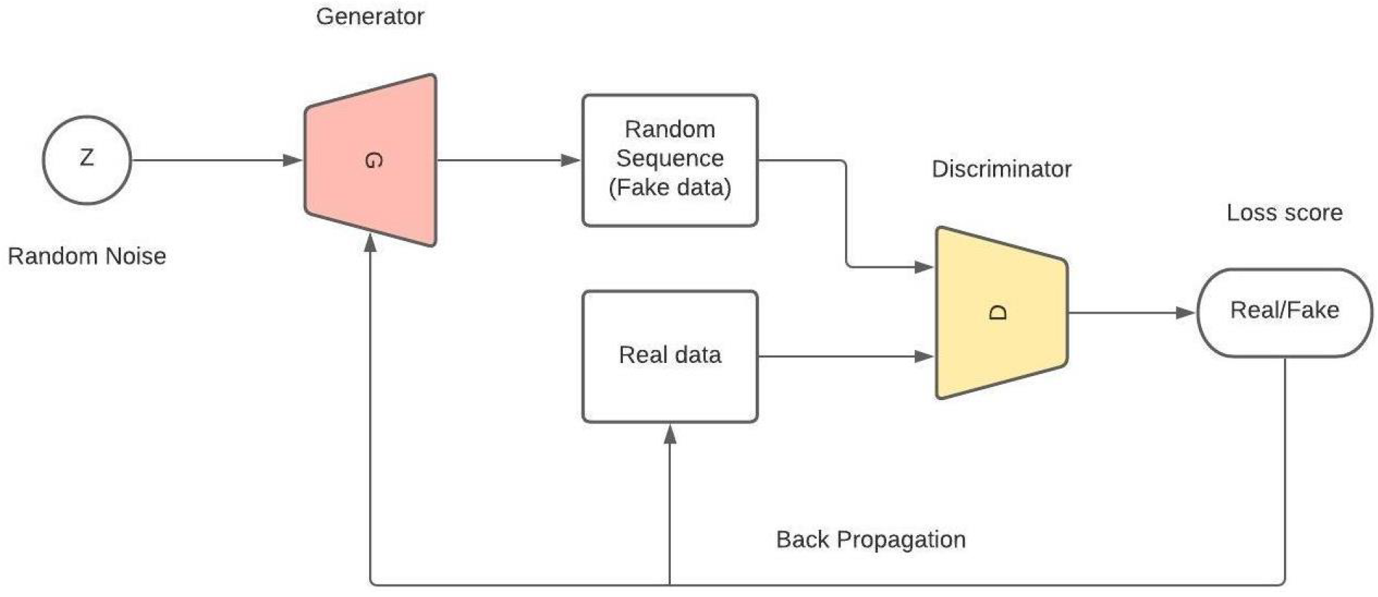
3.1. GAN Conceptual Framework

Generative adversarial Networks (GAN) are class of machine learning/deep learning framework which are used to train generative models.These networks are fascinating enough due to its past implementations to apply on the critical infrastructure areas like energy systems, agriculture and other industries. Which is why it is worth studying the use of GAN on the major scales. Using Generative adversarial networks, we can produce synthetic data which is indistinguishable from the original data in terms of data attributes by passing real data sequence and random noise as an input to the framework. Traditional GAN framework consists of two Neural networks linked to each other, namely, Generator network and Discriminator network. Both generator and discriminator network are setup with initial weights to respective layers. Generator Network takes random noise as an input and generates sequence of data, which is passed onto the Discriminator network. The Discriminator network accepts two inputs, one is data sequence produce by generator and other is the sequence of real data. Further, the discriminator network is trained on real sequence and performs the task to classifies the sequence produce by generator to be the real one or the fake one. Both the networks have respective loss function associated with it, which produces the loss or error score at the end of each forward pass through network. Calculated error score is then back propagated through the entire network and respective layer weights are updated. After which the same process is repeated again, this entire forward pass followed by back propagation results in one iteration. In order for GAN to learn the data sequence and model the framework to produce synthetic data with similar characteristics, it has to run through several thousands iterations.
Traditional GAN framework (in Figure 1) is not proven to be effective method, when working with time series data. Generative model should be able to capture the dynamic behaviour, sequence and pattern variation of time series data with respect to various variables. Further its effectiveness is determined by how it manages to maintain those relationships among the variables across the time while synthetic data generation. Acquired energy consumption data is recorded for whole 2020 year and have time as one of the attributes and hence can be classified as time-series data. In order to process energy data, it is crucial to maintain the relationship between the latent vector in the feature dimension. Realizing stated condition, researcher yoon and et al. created the TimeGAN in their research [31] and implemented it on Stock exchange data.

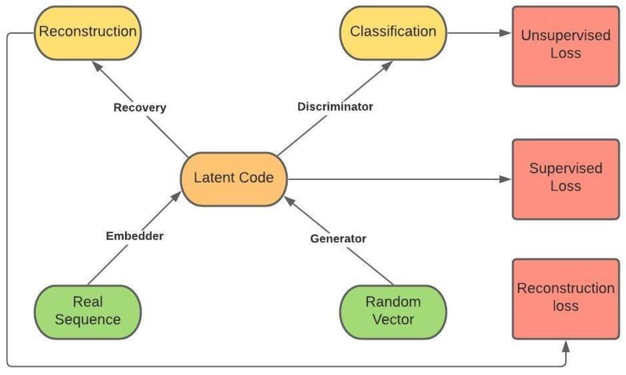
3.2. Proposed Model: Time Variant GAN

As mentioned previously, generative adversarial networks consist of two neural networks, namely, Generator and Discriminator. However, in addition to generator and discriminator, two new networks were introduced in the model which are known as embedding network and recovery network, together these two new networks are called auto encoders. These auto encoders are integral part of proposed model, since these networks are responsible to capture the unknown locality of time series data. Finally, to complete the development of the model, RMSProp optimizer was used which was configured with learning rate of 0.001, decay of 0.9 and momentum of 0.01 as a part of network initialization. overall, described neural network configuration embedded on top of the traditional GAN network integrated with auto encoders develops novel solution to generate synthetic energy data. The time variant GAN is designed to capture features of the real data along with the complex dynamics of those features over the time. The newly introduced embedding network provides reversible mapping between features and latent representation.Embedding network along with recovery network maintains the relationship between latent vectors and features in latent space, while the work of generator and discriminator network remains the same. Similar to the traditional GAN, the generator and discriminator are associated with respective loss function, also known as unsupervised loss. In addition to the unsupervised loss, the model is configured with two more loss functions, known as supervised loss and reconstruction loss, which are associated with auto encoders. The overall architecture overview of the model is shown in Figure 2.
Four Networks-
  • Generator—Generates the data sequence
  • Discriminator—Classifies the data sequence as real or fake
  • Embedding Network—provides reversible mapping between features and latent representation
  • Recovery—provides mapping between feature and latent space
Three types of Losses-
  • Unsupervised Loss—loss function with respect to generator and discriminator network (min-max)
  • Supervised Loss—How well generator calculate next time data in latent space
  • Reconstruction Loss—Compares reconstructed data with original, refers to auto encoders
While calculating supervised loss, model captures the conditional distribution within data with respect to time by supervising original data. Also, this model generates static and sequential data at the same time and passed onto the embedding networks to provide assistance in calculating the next time data in latent space. This technique proven to be more stable training process while training time series data as shown in the evaluation part of this report, further, it is less sensitive to hyperparameter changes as compared to other GANs.

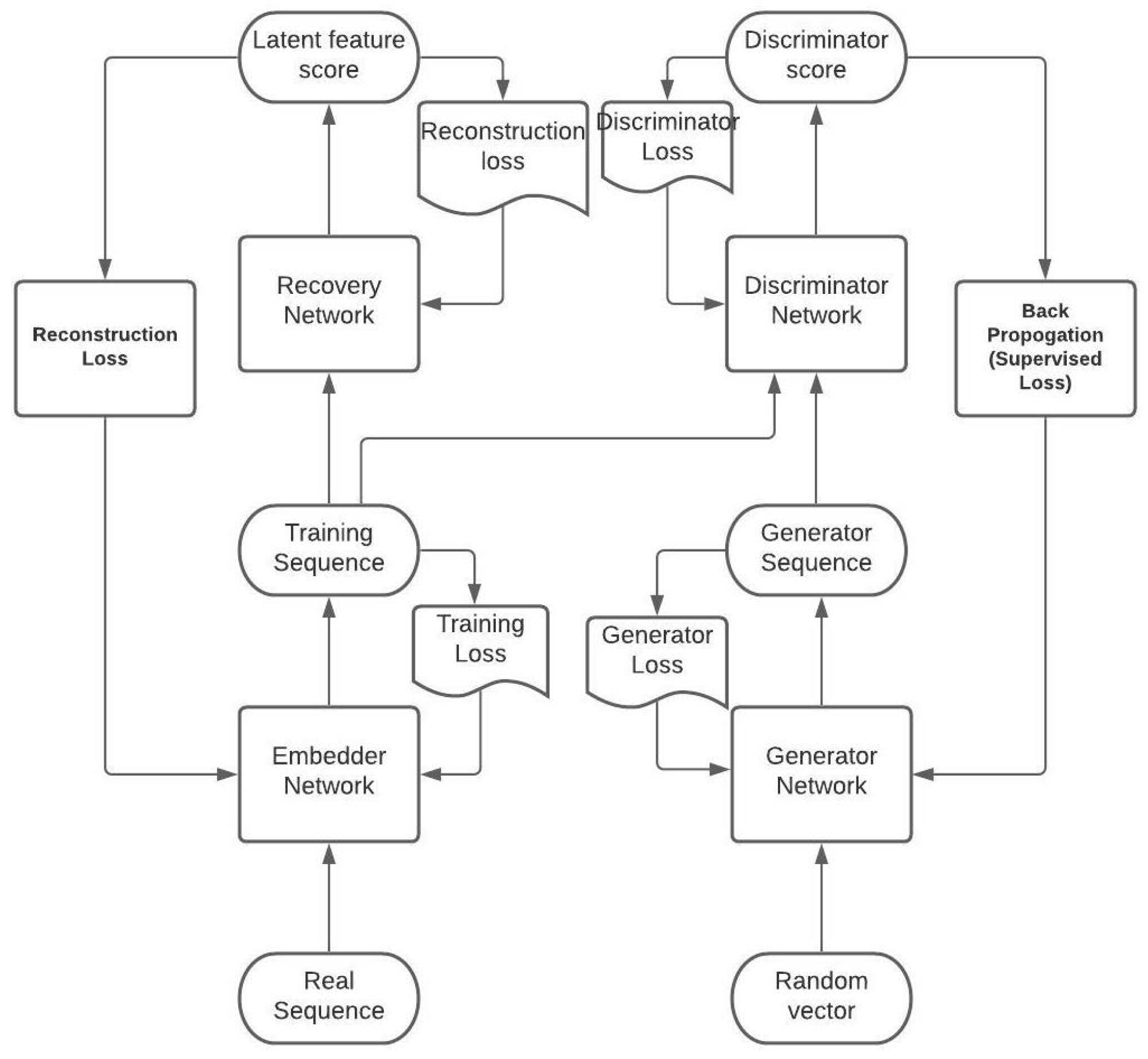
Time GAN Training Phases

Time GAN framework training is divided into 3 folds,
  • Train Autoencoders (embedder and recovery) with given sequential data for optimum reconstruction
  • Train supervisor using real sequence data to capture behavior of historical data
  • Train all 4 networks simultaneously while minimizing Loss functions
Generator take random noise as an input and produces synthetic data as an output. unlike traditional GAN instead of producing data sequence in feature space, Time GAN produces it in an embedding space. Random noise passed to generator function is nothing but the random vector sampled using Gaussian distribution. Overall, Generating function takes a tuple of static and temporal latent vectors to produce synthetic latent vectors in an embedding space. The task of reversible mapping between features and latent representation is carried out in this step and Supervised loss is calculated. In the next step, Discriminator networks receives static and temporal codes from embedding space and performs classification, as a result of which, value of unsupervised loss is acquired. Further, the discriminator network is also associated with another loss value known as discriminator loss. This loss is calculated based on how well the discriminator network training is completed with original data. This loss function is then contributes to fine tune the discriminator network by updating the layer weights to optimum solution, which helps discriminator network to perform unbiased classification between fake data and original data. The latent codes from embedding space is forwarded to recovery network for reconstruction of features in latent space and respective reconstruction loss is produced. All the three losses are back propagated through entire network and helps to fine tune the weights that are assigned in different layers, so as to generate more realistic data. Recurrent networks and bi-directional recurrent networks are used for generator and discriminator, respectively. At generator network, technique known as gradient ascent is used to find global maxima, while, on the contrary, gradient descent is used at the discriminator function to reach the global minima. In other words, generator network tries to minimize the adversarial loss, while discriminator function tries to maximize it in their min-max game. This process is carried out in loop for several number of iterations, until the model learns the dynamic energy consumption pattern and produces synthetic data possessing similar characteristics as that of real data. The flow of training process is shown in Figure 3.
Algorithm:
1. Start Auto encoder training on real data
  • Step 1: Embedder <- Real data sequence vector as an input
  • Step 2: Supervised Loss <- Loss calculated from Embedder network
  • Step 3: Recovery <- Data sequence vector from Embedder in latent space
  • Step 4: Reconstruction Loss <- Loss calculated from Recovery network
  • Step 5: Embedder <- Supervised Loss from step 2 & Reconstruction Loss from step 4; to update layer weights
  • Step 6: Embedder <- Next data sequence vector
  • Step 7: Repeat Step 1 to Step 6 for several iterations
2. Train Discriminator and generator
  • Step 8: Generator <- Random noise vector as an input(fake data)
  • Step 9: Generator Loss <- Loss calculated on generated sequence
  • Step 10: Generator <- Generator Loss, to update layer weights
  • Step 11: Discriminator <- Output from Generator network and original data sequence
  • Step 12: Discriminator Loss <- Loss calculated based on discriminator training on original data
  • Step 13: Discriminator <- Discriminator Loss; to update layer weights
  • Step 14: Supervised Loss <- Loss calculated at discriminator based on how well it categorized fake data from real data
  • Step 15: Generator <- Supervised Loss, to update layer weights again
  • Step 16: Repeat step 8 to Step 15 for several iterations
3. Train Auto encoders, Generator and Discriminator Simultaneously
  • Step 17: Repeat all the steps for several Iterations

4. Artefact Development Approach

The proposed artefact is to be implemented on the energy consumption dataset to produce the synthetic energy data. However, as described in Section 3, Time GAN framework is complex and could result in overfitting or underfitting depending on the number of data points and other characteristics and network parameters. Hence, before actual implementation, it is crucial to understand the dataset and neural network parameters associated with the model. Further, it is important to understand system requirements and tools necessary to perform complex computation smoothly.

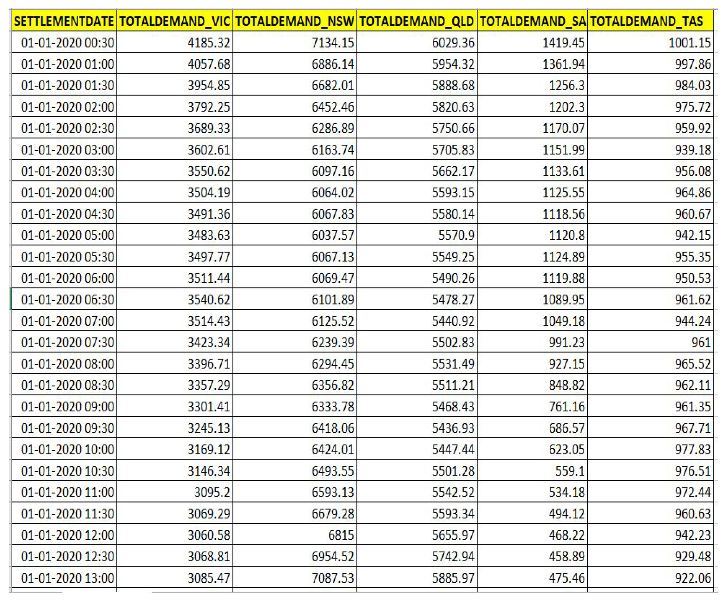
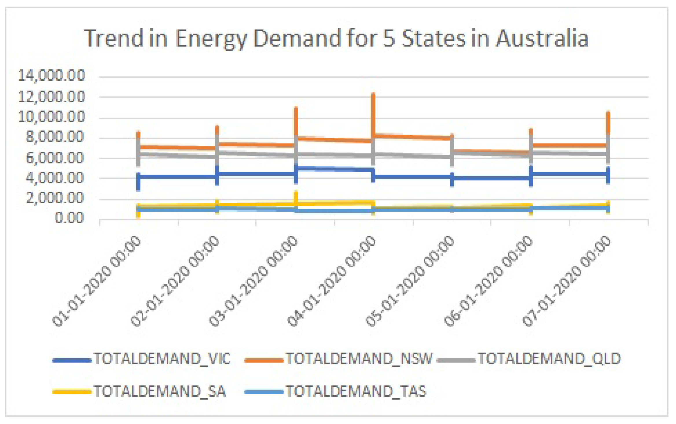
4.1. Dataset Information

Energy consumption dataset is acquired from the “AEMO—Aggregated Price and Demand data” website (https://aemo.com.au/en/energy-systems/electricity/national-electricity-market-nem/data-nem/aggregated-data, accessed on 11 April 2021). Website contains monthly energy consumption data for various states of Australia. For this project, energy data is collected for whole 2020 year for the states Victoria, New South Wales, South Australia, Queensland and Tasmania, as described in Table 3.
Each attribute provides value of energy power consumption for respective states in Australia. Further, Figure 4 provides an overview of the energy data.The data is collected for every 30 min interval from 1 January 2020 00:00 to 1 January 2021 00:00 with total data points equals to 17,568. It has been observed that data follows the similar trend when observed for single day. Overall, the demand for New South Wales is highest throughout the year followed by Queensland. The state of Victoria comes in third place, while the energy demands are lower in South Australia in comparison to Victoria. The least energy demand is recorded for Tasmania. The distribution and trend in energy demand is showcased in Figure 5, in which the data for seven consecutive days is compared for all the five states. Similar trend is observed for rest of the datapoints.

4.2. System and Tool Requirements

The dataset holding energy consumption data is stored is csv format and used as an input to GAN model for model training purpose. We have used python programming language and Google Collaboratory to execute and implement Time GAN framework. GPU environment has been setup to improve processing and reduce execution time. Table 4 describes the technological requirements that has been setup for this project.

4.3. Neural Network Parameters and Prerequisites

The energy consumption data is pre-processed before passed down for model training as an input to Time GAN. The dataset is arranged in chronological order of the time by flipping over, so that energy consumption data is arranged from latest to oldest date. Further, the data is normalized to the values between 0 and 1 using ‘Min-Max scaler’. In the next step, the data cut into smaller payloads as per the provided sequence length and afterwards it is arranged in the random permutations. Once all of the stated steps of data processing is completed, energy data is ready to passed on to the model for training. In addition the data, network parameters are also configured and forwarded for execution to achieve optimal model training. These parameters includes, sequence length, module, number of hidden dimensions, number of layers in neural network, training batch size and number of iterations. Depending upon the system processor the execution time for the model training will differ, however, in this case, it has been recorded as 3 h on average.

5. Experiments and Evaluation

5.1. Experimental Setup

The system and tools are configured as mentioned in the Section 4.2 to setup an environment for time GAN implementation. In order to write a python code, necessary python libraries are imported. Also the energy consumption data is pre-processed with the sequence length of 24, as stated in Section 5.1. Further, The parameter are configured with the default values as mentioned in Table 5.
Execution code for all the four neural networks is defined using respective python libraries and functions. Further, ‘Sigmoid’ and ‘tanH’ activation functions are used for respective layers in the neural networks, while, ‘ReLu’ activation function is setup to train the whole GAN network simultaneously. Optimizers such as ‘Adam’, ‘RMSProp’ and ‘GradientDecentOptimizer’ were used in different scenarios in opposed to the proposed model. Hyper-parameters were setup with learning rate, decay rate and momentum to improve the results Time variant GAN model. To achieve the optimal results, stated hyper-parameters were tuned in different scenarios as mentioned in the Table 5. Along with the proposed model, six scenarios were executed by with different combination of hyper-parameters and their results are compared against the proposed model by set of standards mentioned in Section 5.2 model evaluation. Table 6 provides brief information on all of the six experiments as well as details of the proposed model.

5.2. Model Evaluation

We compared the results of all the experiments with proposed model of Time variant GAN. The performance of the model has been measured using various evaluation metrics used in quantitative analysis as described in Section 5.2.1. Also, to better understand results visualization techniques are used. The results are showcased using PCA and TSNE graphs with two component dimensionality reduction. Further, quality of generated data is evaluated using train-on-synthetic and test-on-real(TSTR) methodology. Finally, the statistics on generated and real data has been compared which depicts the comparison of characteristics of original data against generated data using mean, SD, minimum value, maximum value and interquartile range ranges.

5.2.1. Quantitative Evaluation

Quantitative evaluation of the model is carried out using eight quantitative metrics. These are discriminative score, predictive score Accuracy, precision, recall, f1-score, cohens kappa and ROC AUC. All metrics are calculated based on TSTR method, 2-layer LSTM time series classification model is used to trained on synthetic sequence of data, in order to differentiate the real data sequences from the fake ones. Each of the original data point was labeled while the synthetic data point left unlabeled and RNN classifier is used to trained so as to distinguish between them. Finally, respective error value is calculated and reported as discriminative score. Further, values of accuracy, precision, recall, f1-score, cohens kappa, ROC AUC is calculated based on the performance of RNN classifier. On the other hand, to verify whether the proposed time variant GAN model was able to capture the temporal dynamics and conditional distribution over time, We calculated predictive score. Again, two layer LSTM sequence predicting model was trained using synthetic data and used to predict the temporal vectors in the next step based on the previous step. Performance of prediction was measured using mean absolute error (MAE) and reported as a predictive score of the model. In order for describing model to be a better one, both discriminative score and predictive score should be close to 0.

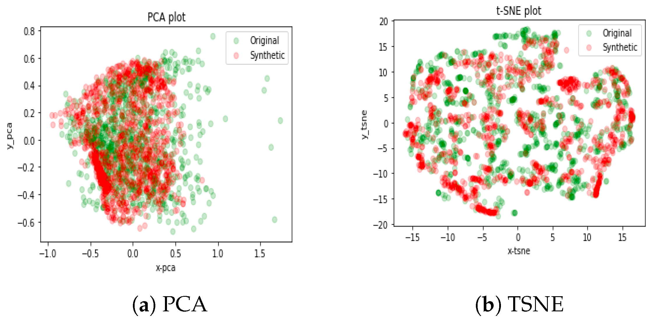
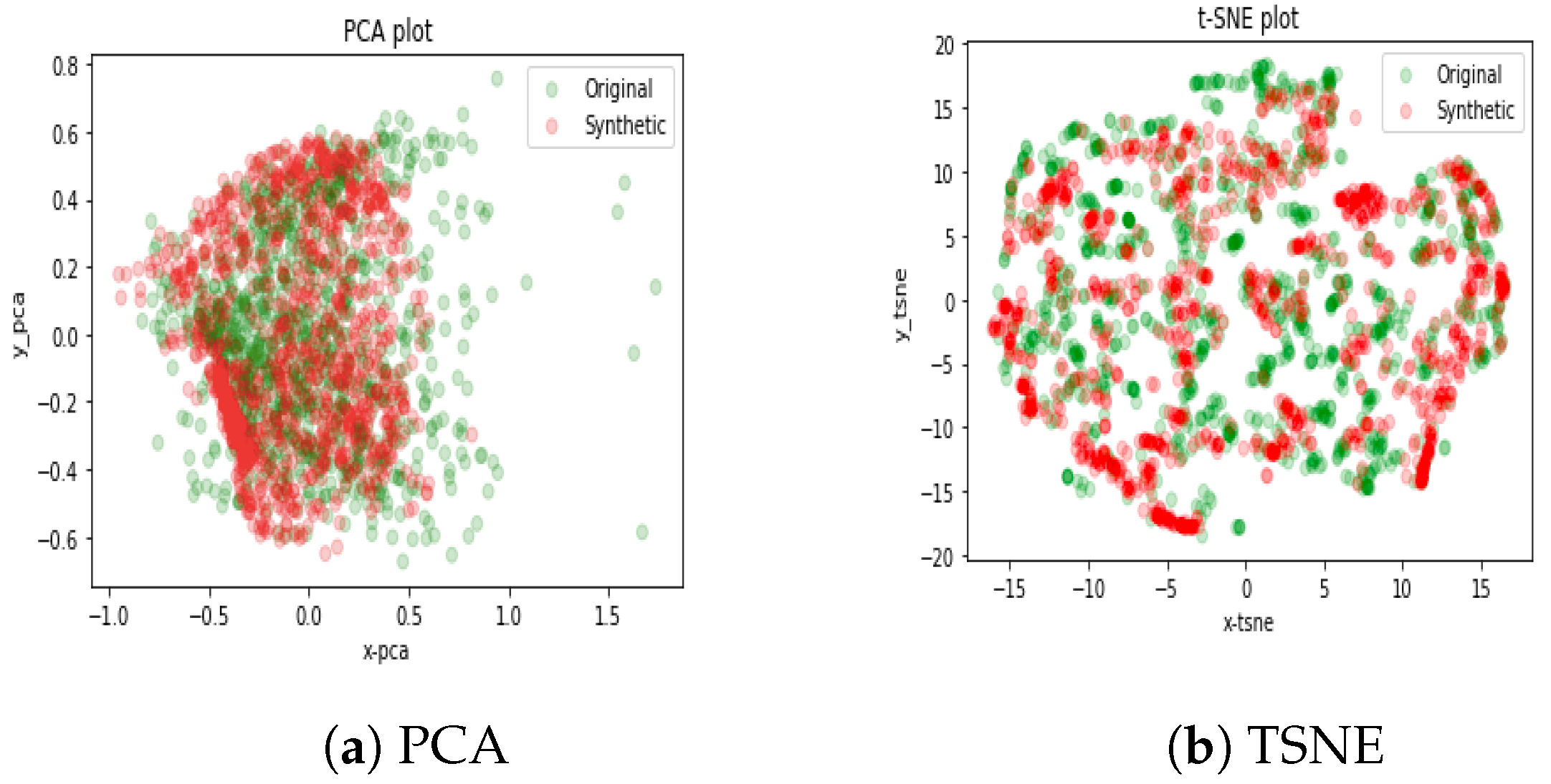
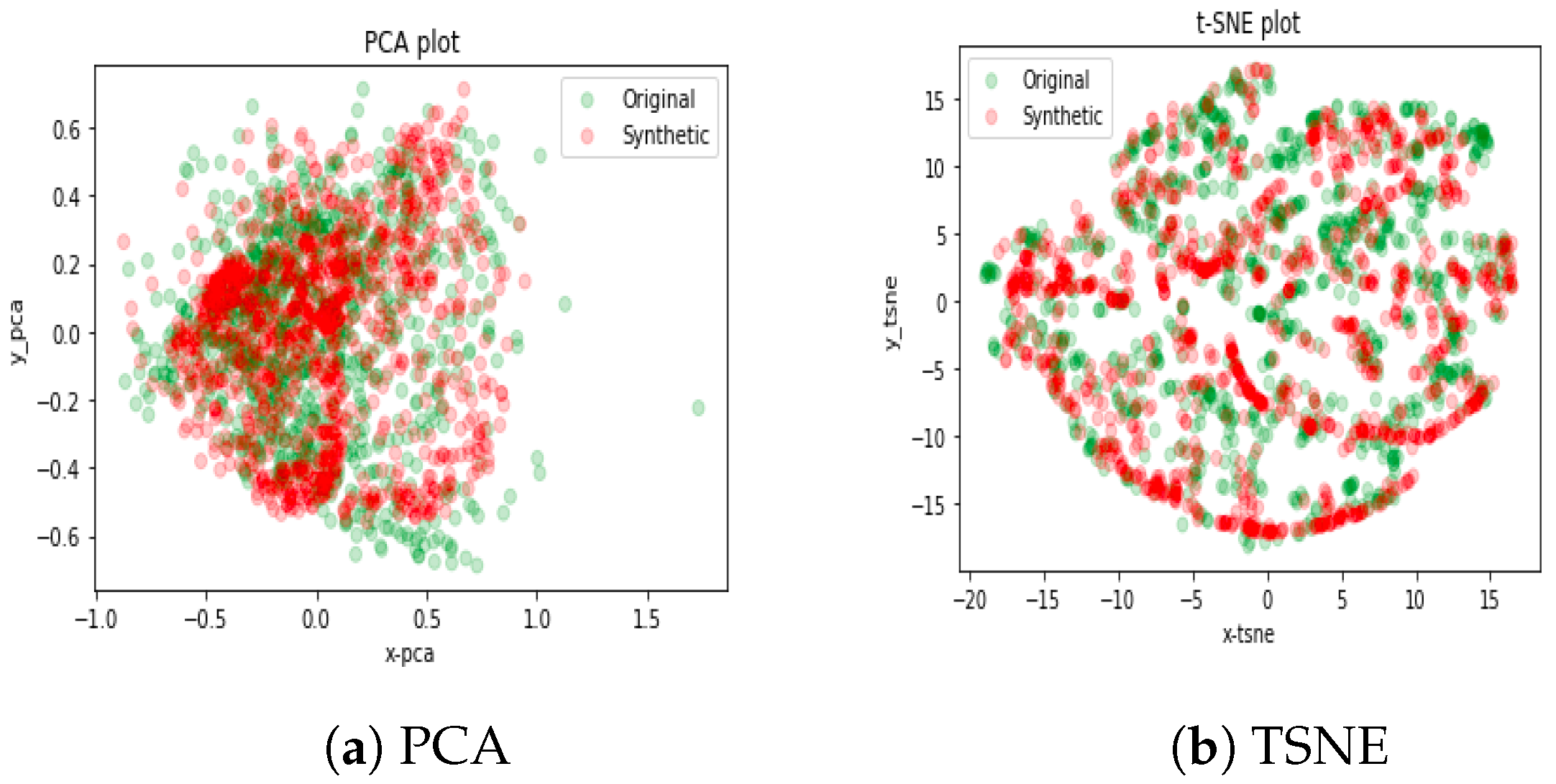
5.2.2. Visualization and Graphs

Finally, the original data points and synthetic data points for energy consumption data are plotted on two-dimensional space using PCA and TSNE graphs by performing dimensionality reduction with two components. Both PCA and TSNE graphs were plotted for all experiments and results are compared in Section 6.

5.2.3. Other Evaluation Methods

The quality of generated data is evaluated based on three factors.
  • How well generated samples are distributed across the real data?
  • Are generated samples are indistinguishable from the real data?
  • How effectively Generated samples can be used for predictive purposes, likewise real data?
Further, qualitative analysis is done using train-on-synthetic, test-on-real (TSTR) method. In this method, model is trained on synthetic data and its accuracy is calculated by performing tests on real data. We have used, two Layer LSTM model for the training purpose using synthetic energy consumption data, while testing accuracy is calculated using original energy consumption data.
Furthermore, statistics measures such as mean, SD and interquartile range ranges were calculated for the subset of original data and synthetic data, and reported for comparison purposes, since it provides a strong platform in comparing the quality of the synthetic data.

6. Results & Discussion

Overall, in order to evaluate the results for all the experiments, the accuracy of synthetic data with respect to real data is presented based on similarity index. Further, train on synthetic data and test on real data method is used to calculate predictive score, which adds up to effectiveness of model. Finally, the results are visualized using graphs along with PCA and TSNE with two components.

6.1. Interpretation of Results

The results of the experimental evaluation is showcased in ‘Table 7: Experimental Results’. This table contains the value for following metrics, Discriminator score, Predictive score, Accuracy, precision, recall, f1-score, cohens kappa and ROC AUC. Discriminator score and Predictive score depicts the MAE values with respect to original data sequence and generated data sequence, while other measures showcases similarity index between respective data sequence.
After the training of Time GAN model, the synthetic data was generated, which is evaluated using stated quantitative metrics. In order to perform quantitative analysis, at first the vector sequences in original data is labeled as 1, while the vector sequence of synthetic data is labeled as 0. Further, two layer LSTM model was trained using these vector sequences from original as well as synthetic data and then classifier was used to classifies them for the inline vector sequences and error rate was calculated. Now, specifically for the Time GAN model, if the generated data is equivalent to the original data, then the discrimination accuracy for the model should be low. In other words, if the model is able to generate the data fairly indistinguishable from the original data then value of the stated metrics should be less and close to 0, instead of being close to 1. Hence, lower is the values of all the metrics better is the Time GAN model.

6.2. Performance Comparison

As mentioned previously, in order to for the described model to be better, both discriminative score and predictive score should be close to 0. Comparison of experimental results of proposed model in terms of qualitative and quantitative metrics with other scenarios is presented in Table 7.
The values of all the metrics are recorded in Table 7 for all the scenarios. It can be seen that the proposed model with RMSProp Optimizer is showing better performance than other experimental setup, since the discriminative score and predictive score are close to zero, which are 0.06830 and 0.0744, respectively. While, for Adam optimizer with learning rate 0.0001, the scores are 0.1132 and 0.0774 respectively. Similarly, for experiment two, it is recorded as 0.4757 and 0.1509 for Adam optimizer with default learning rate. Higher value of scores are recorded for scenarios 3, 5 and 6. However, we wanted discriminator score and predictive score to be less, since both the scores are measured in terms of error. On the other hand, fairly similar values are observed for scenario four in which RMSProp optimizer is used with learning rate of 0.001. However, they are still higher than proposed model. Overall, the best optimal values for the metrics are recorded for the proposed solution, hence is outperforms the other models.

6.3. Statistical Comparison

This section compares the statistics on subset of original data and generated data. Comparison includes measures such as mean value, min value, max value and likewise other standards. The Table 8 below compares the value of mean, standard deviation, min, max and interquartile range for scenario 1, 2 and 3 with the values of proposed model. These calculated values are in normalized form, since our data is standardized using mixmaxscaler at the very beginning. Clearly, it can be seen that the values of original data and generated data for proposed model are more equivalent to each other as compared to other three scenarios. Similarly, in Table 9, we can notice that proposed model is more statistically significant in comparison to the scenarios 4, 5 and 6. This statistical comparison created more robust platform of quality measure of generated synthetic energy data.

6.4. Visualization

Further, to perform more robust comparison, PCA and TSNE plots are produced for the proposed model along with all the experiments. From the graphs below, it can be seen that, in the PCA and TSNE plots for the proposed model in Figure 6, generated data sequence is following the pattern of original data sequence more closely, as compared to other models. Also, in Figure 7, scenario 1 no pattern is produced as a result of underfitting. While, for the rest of the experiments as shown in Figure 8, Figure 9 and Figure 10, model seems to have produce compatible synthetic data. However, when considering all the evaluation methods, proposed model has definitely produced good results and able to generate synthetic energy data with similar characteristics with the real data.
The code execution, original energy dataset obtained from AEMO website and Synthetic energy dataset generated as a result of this research implementation can be viewed using following link—Available online: https://github.com/ShashankAsre/TimevariantGAN-AEMO-dataset (accessed on 1 December 2021).

7. Conclusions & Future Work

In this research project, we were able introduce the novel time variant GAN solution, built using RMSProp optimizer on top of the existing framework. We were able to train the proposed model with energy consumption dataset acquired from AEMO website and were able to produce the synthetic energy consumption data, possessing similar characteristics as that of real data. Further, using metrics such as discriminative score, predictive score, accuracy, precision and other scores, we were able to provide quantitative evaluation of the model. PCA and TSNE graphs helped in showcasing the similar trends between the synthetic data and real data, which provided more robust evidence in proving the effectiveness of the proposed model. We were able to prove that Time variant GAN model is more effective in learning the dynamic behaviour of time series data and able to replicate the same behaviour in synthetic data. Overall, Time variant GAN has shown great improvements over the state-of-art frameworks, by leveraging the contribution of jointly trained neural networks and respective loss functions, and has shown the significant contribution in the field of energy.

Future Work

In the future, generated synthetic data could be used to create various solution for energy optimization and help researcher to develop novel methods to save energy, without having to worry about the customer privacy issues associated with energy consumption data. On the implementation level, the model can be improved further by optimizing the embedding and recovery network, so as to increase its tendency to capture the temporal behaviour of the data over the time, while effectively performing the reversible mapping between features and latent representation. Further, model performance can be improved by hyperparameter tuning, changing batch size, adding extra layers in neural network, implementing possible optimizers and using dropout values.

Author Contributions

Conceptualization, A.A. and S.A.; methodology, S.A.; software, S.A.; validation, S.A. and A.A.; formal analysis, S.A.; investigation, S.A.; resources, A.A.; data curation, S.A.; writing—original draft preparation, S.A.; writing—review and editing, A.A.; visualization, S.A.; supervision, A.A.; project administration, A.A. All authors have read and agreed to the published version of the manuscript.

Funding

This research received no external funding.

Institutional Review Board Statement

Not applicable.

Informed Consent Statement

Not applicable.

Data Availability Statement

The data can be found at https://github.com/ShashankAsre/TimevariantGAN-AEMO-dataset (accessed on 1 December 2021).

Conflicts of Interest

The authors declare no conflict of interest.

References

  1. Anwar, A.; Mahmood, A.N.; Tari, Z. Identification of vulnerable node clusters against false data injection attack in an AMI based Smart Grid. Inf. Syst. 2015, 53, 201–212. [Google Scholar] [CrossRef]
  2. Sestrem Ochôa, I.; Augusto Silva, L.; de Mello, G.; Garcia, N.M.; de Paz Santana, J.F.; Quietinho Leithardt, V.R. A Cost Analysis of Implementing a Blockchain Architecture in a Smart Grid Scenario Using Sidechains. Sensors 2020, 20, 843. [Google Scholar] [CrossRef] [PubMed] [Green Version]
  3. Suzin, J.C.; Zeferino, C.A.; Leithardt, V.R.Q. Digital Statelessness—New Trends in Disruptive Technologies, Tech Ethics and Artificial Intelligence; Springer International Publishing: Berlin/Heidelberg, Germany, 2021. [Google Scholar] [CrossRef]
  4. Reda, H.T.; Anwar, A.; Mahmood, A.N.; Tari, Z. A Taxonomy of Cyber Defence Strategies Against False Data Attacks in Smart Grid. arXiv 2021, arXiv:2103.16085. [Google Scholar]
  5. Husnoo, M.A.; Anwar, A.; Hosseinzadeh, N.; Islam, S.N.; Mahmood, A.N.; Doss, R. False Data Injection Threats in Active Distribution Systems: A Comprehensive Survey. arXiv 2021, arXiv:2111.14251. [Google Scholar]
  6. Husnoo, M.A.; Anwar, A.; Chakrabortty, R.K.; Doss, R.; Ryan, M.J. Differential Privacy for IoT-Enabled Critical Infrastructure: A Comprehensive Survey. IEEE Access 2021, 9, 153276–153304. [Google Scholar] [CrossRef]
  7. Baasch, G.; Rousseau, G.; Evins, R. A Conditional Generative adversarial Network for energy use in multiple buildings using scarce data. Energy AI 2021, 5, 100087. [Google Scholar] [CrossRef]
  8. Fekri, M.N.; Ghosh, A.M.; Grolinger, K. Generating Energy Data for Machine Learning with Recurrent Generative Adversarial Networks. Energies 2020, 13, 130. [Google Scholar] [CrossRef] [Green Version]
  9. Goodfellow, I.J.; Pouget-Abadie, J.; Mirza, M.; Xu, B.; Warde-Farley, D.; Ozair, S.; Courville, A.; Bengio, Y. Generative Adversarial Nets; Cornell University: New York, NY, USA, 2014. [Google Scholar]
  10. Viel, F.; Augusto Silva, L.; Leithardt, V.R.Q.; De Paz Santana, J.F.; Celeste Ghizoni Teive, R.; Albenes Zeferino, C. An Efficient Interface for the Integration of IoT Devices with Smart Grids. Sensors 2020, 20, 2849. [Google Scholar] [CrossRef]
  11. Li, Y.; Wang, Q.; Zhang, J.; Hu, L.; Ouyang, W. The Theoretical Research of Generative Adversarial Networks: An Overview. Neurocomputing 2021, 435, 26–41. [Google Scholar] [CrossRef]
  12. Padhani, A.; Mirza, B.; Khan, D.B.; Syed, T.Q. Deep Generative Models to Counter Class Imbalance: A Model-Metric Mapping with Proportion Calibration Methodology. IEEE Access 2021, 9, 55879–55897. [Google Scholar] [CrossRef]
  13. Shao, G.; Gao, M.; Liu, T.; Li, L. DuCaGAN: Unified Dual Capsule Generative Adversarial Network for Unsupervised Image-to-Image Translation. IEEE Access 2020, 8, 154691–154707. [Google Scholar] [CrossRef]
  14. Cai, Y.; Yu, X.Z.; Li, F.; Xu, P.; Li, Y.; Li, L. Dualattn-GAN: Text to Image Synthesis With Dual Attentional Generative Adversarial Network. IEEE Access 2019, 7, 183706–183716. [Google Scholar] [CrossRef]
  15. Wang, D.; Dong, L.; Wang, R.; Yan, D.; Wang, J. Targeted Speech Adversarial Example Generation with Generative Adversarial Network. IEEE Access 2021, 8, 124503–124513. [Google Scholar] [CrossRef]
  16. Liu, J.; Tian, Y.; Zhang, R.; Sun, Y.; Wang, C. A Two-Stage Generative Adversarial Networks with Semantic Content Constraints for Adversarial Example Generation. IEEE Access 2020, 8, 205766–205777. [Google Scholar] [CrossRef]
  17. Oluwasanmi, A.; Muhammad Umar Aftab, A.A.S.; Jackson, J.; Kumeda, B.; Qin, Z. Attentively Conditioned Generative Adversarial Network for Semantic Segmentation. IEEE Access 2020, 8, 31733–31741. [Google Scholar] [CrossRef]
  18. Yang, Y.; Dan, X.; Qiu, X.; Gao, Z. FGGAN: Feature-Guiding Generative Adversarial Networks for text generation. IEEE Access 2020, 8, 105217–105225. [Google Scholar] [CrossRef]
  19. Wu, E.; Roy, H.; Welsch, E. Dual Autoencoders Generative Adversarial Network for Imbalanced Classification Problem. IEEE Access 2020, 8, 91265–91275. [Google Scholar] [CrossRef]
  20. Liu, Z.; Yin, X. LSTM-CGAN: Towards Generating Low-Rate DDoS Adversarial Samples for Blockchain-Based Wireless Network Detection Models. IEEE Access 2021, 9, 22616–22625. [Google Scholar] [CrossRef]
  21. Liu, J.; Zhang, Y.Z.; Lei, Y.; Li, J.; Zhang, M.; Yang, X. Recent Advances of Image Steganography with Generative Adversarial Networks. IEEE Access 2020, 8, 60575–60597. [Google Scholar] [CrossRef]
  22. Jiang, W.; Hong, Y.; Zhou, B.; He, X.; Cheng, C. A GAN-Based Anomaly Detection Approach for Imbalanced Industrial Time Series. IEEE Access 2019, 7, 143608–143619. [Google Scholar] [CrossRef]
  23. Sun, Y.; Yu, W.; Chen, Y.; Kadam, A. Time Series Anomaly Detection Based on GAN. In Proceedings of the 2019 Sixth International Conference on Social Networks Analysis, Management and Security (SNAMS), Granada, Spain, 22–25 October 2019. [Google Scholar] [CrossRef]
  24. Zhu, G.; Zhao, H.; Liu, H.; Sun, H. A Novel LSTM-GAN Algorithm for Time Series Anomaly Detection. In Proceedings of the 2019 Prognostics and System Health Management Conference (PHM-Qingdao), Qingdao, China, 25–27 October 2019. [Google Scholar] [CrossRef]
  25. Luer, F.; Mautz, D.; Bohm, C. Anomaly Detection in Time Series using Generative Adversarial Networks. In Proceedings of the 2019 International Conference on Data Mining Workshops (ICDMW), Beijing, China, 8–11 November 2019. [Google Scholar] [CrossRef]
  26. Choi, Y.; Lim, H.; Choi, H.; Kim, I.J. GAN-Based Anomaly Detection and Localization of Multivariate Time Series Data for Power Plant. In Proceedings of the 2020 IEEE International Conference on Big Data and Smart Computing (BigComp), Busan, Korea, 19–22 February 2020. [Google Scholar] [CrossRef]
  27. Smith, K.; Smith, A.O. Conditional Gan for Timeseries Generation. arXiv 2020, arXiv:2006.16477. [Google Scholar]
  28. Hyland, S.L.; Esteban, C.; Rätsch, G. Real-Valued (Medical) Time Series Generation with Recurrent Conditional Gans. arXiv 2017, arXiv:1706.02633. [Google Scholar]
  29. Derek, S. MTSS-GAN: Multivariate Time Series Simulation Generative Adversarial Networks; SSRN: Rochester, NY, USA, 2020. [Google Scholar]
  30. Husein, A.; Arsyal, M.; Sinaga, S.; Syahputa, H. Generative Adversarial Networks Time Series Models to Forecast Medicine Daily Sales in Hospital. Sinkron 2019, 3, 112–118. [Google Scholar] [CrossRef]
  31. Yoon, J.; Jarrett, D.; van der Schaar, M. Time-Series Generative Adversarial Networks; Curran Associates, Inc.: New York, NY, USA, 2019. [Google Scholar]
  32. Schmidhuber, J. Generative adversarial networks are special cases of artificial curiosity (1990) and also closely related to predictability minimization (1991). Neural Netw. 2020, 127, 58–66. [Google Scholar] [CrossRef]
  33. Schmidhuber, J. Learning factorial codes by predictability minimization. Neural Comput. 1992, 4, 863–879. [Google Scholar] [CrossRef]
Figure 1. Traditional GAN Framework.
Electronics 11 00355 g001
Figure 2. Time variant GAN Framework [31].
Electronics 11 00355 g002
Figure 3. Time variant GAN training process.
Electronics 11 00355 g003
Figure 4. AEMO data- Energy Consumption Data.
Electronics 11 00355 g004
Figure 5. Energy Demand comparison for 7 consecutive days.
Electronics 11 00355 g005
Figure 6. Proposed Model—RMSProp (lr = 0.001, momentum = 0.01, decay rate = 0.9).
Electronics 11 00355 g006
Figure 7. Scenario 1—Adam (lr = 0.001).
Electronics 11 00355 g007
Figure 8. Scenario 2—Adam (lr = 0.0001).
Electronics 11 00355 g008
Figure 9. Scenario 3—Adam (lr = default).
Electronics 11 00355 g009
Figure 10. Scenario 4—RMSProp (lr = 0.001, decay = 0.9).
Electronics 11 00355 g010
Table 1. List of Abbreviations.
AbbrFull formDefinition
GANGenerative
Adversarial
Networks
GAN are Machine Learning model consist
of two Neural Networks which competes
each other to increase accuracy of their prediction
PCAPrincipal
Component
Analysis
PCA is dimensionality-reduction method used to
reduce the dimensionality of large datasets
TSNEt-distributed
stochastic neighbor
embedding
It is a statistical method for visualizing high
dimensional data by giving each datapoint
a location in a two or three-dimensional map
PMUPhasor
measurement
Units
A phasor measurement unit (PMU) is a device used to
estimate the magnitude and phase angle of an electrical
phasor quantity such as voltage or current
OTOperation
Technology
It is hardware and software that detects or causes a
change, through the direct monitoring and/or control
of industrial equipment, assets, processes and events.
FDIFalse Data
Injection Attacks
FDI compromises sensor readings by
introducing errors into calculations of state variables
and values.
DOSDenial-of-service
attack
It is an attack meant to shut down network,
making it inaccessible to its intended users
AUCArea
Under
Curve
AUC is the measure of the ability of a classifier to
distinguish between classes and is used as a summary
of the ROC curve
ROCReceiver
Operating
Characteristic
ROC is a graph showing the performance of a
classification model at all classification thresholds.
AEMOAggregated
Price and
Demand data
AEMO is a website that contains monthly
energy consumption data for various states of
Australia
TSTRTrain on
Synthetic
Test on Real
A method in which model is trained on Synthetic
data and accuracy is tested on the real data
Table 2. Relevant Literatures.
Summarized Literatures
Article TitleVenueY.O.PAuthorsApplication AreaAlgorithm UsedDatasetsMetrics
Deep generative models to counter class imbalance: a model-metric mapping with proportion calibration methodology [12]IEEE2021BEHROZ MIRZA, DANSIH HAROON, BEHRAJ KHAN, ALI PADHANI, TAHIR Q. SYEDclass imbalance-Machine LearningGAN, VAM, RBMCreditcard-fraud detection dataset Give-mesome-credit dataset Protein-homo dataset Skin-no-skin dataset Anti-moneylaundering- casesPrecision, Recall, F1-score, AUC, G-Mean, Balanced Accuracy
DuCaGAN: Unified Dual Capsule Generative Adversarial Network for Unsupervised Image-to-Image Translation [13]IEEE2020GUIFANG SHAO, MENG HUANG, FENGQIANG GAO, TUNDONG LIU, LIDUAN LIcomputer vision and image processingdual capsule generative adversarial networkCityscapes, Sketch2photo, Day2night, Oil2Chinese, Summer2Winter, Ukiyoe2photo, Vangogh2photo, Surface defect data, DAGM 2007semantic segmentation evaluation, FCN-score, four evaluation criteria, pixel accuracy, mean accuracy, frequency weighted Intersection-Over-Union, mean class Intersection-Over-Union(ClassIOU)
Dualattn-GAN: Text to Image Synthesis with Dual Attentional Generative Adversarial Network [14]IEEE2019YALI CAI, XIAORU WANG, ZHIHONG YU, FU LI, PEIRONG XU, YUELI LI, LIXIAN LIText to Image processingDual Attentional Generative Adversarial Network (DualAttn-GAN)CUB, Oxford-102Inception Score (IS), Fréchet Inception Distance (FID), Human Rank (HR)
Targeted Speech Adversarial Example Generation with Generative Adversarial Network [15]IEEE2020DONGHUA WANG, LI DONG, RANGDING WANG, DIQUN YAN, JIE WANGSpeech processing and generationTraditional generative adversarial network (GAN)SpeechCmd, GTZANSNR (db), PESQ
A Two-Stage Generative Adversarial Networks with Semantic Content Constraints for Adversarial Example Generation [16]IEEE2020JIANYI LIU, YU TIAN, RU ZHANG, YOUQIANG SUN, CHAN WANGImage processing and generationTwo-stage generative adversarial networks (TSGAN)MNIST, CIFAR-10Fréchet Inception Distance (FID), Structural Similarity (SSIM)
Attentively Conditioned Generative Adversarial Network for Semantic Segmentation [17]IEEE2020ARIYO OLUWASANMI, MUHAMMAD UMAR AFTAB, AKEEM SHOKANBI, JEHOIADA JACKSON, BULBULA KUMEDA, ZHIQUANG QINsemantic segmentationAttentively Conditioned Generative Adversarial Network (ACGAN)PASCAL VOC 2012, CamVidpopular mean Intersection over Union (mIoU) technique
FGGAN: Feature-Guiding Generative Adversarial Networks for Text Generation [18]IEEE2020YANG YANG, XIAODONG DAN, XUESONG QIU, ZHIPENG GAOText GenerationFeature-Guiding
Generative Adversarial Networks (FGGAN)COCO dataset, Chinese poetry datasetbilingual evaluation understudy (BLEU) score
Dual Autoencoders Generative Adversarial Network for Imbalanced Classification Problem [19]IEEE2020Ensen Wu, Hongyan Cui, Roy E. WelschFraud DetectionDual Autoencoders Generative Adversarial Networkcredit card transaction datasetrecall, precision, F1-score, Area Under the Curve (AUC), Area Under Precision-Recall Curve (AUPRC)
LSTM-CGAN: Towards Generating Low-Rate DDoS Adversarial Samples for Blockchain-Based Wireless Network Detection Models [20]IEEE2021ZENGGUANG LIU, XIAOCHUN YINblockchain-based protection technologies for DDOS attacksLSTM-CGANslow-header, slow-body, hulk and rudy of iscx-slowdos-2016, Friday datasetError rate, Precision, recall
Recent Advances of Image Steganography with Generative Adversarial Networks [21]IEEE2020JIA LIU, YAN KE, ZHUO ZHANG, YU LEI, JUN LI, MINQING ZHANG, XIAOYUAN YANGImage SteganographyGANCIFAR-100, CelebA, BOSS, Div2k, COCO, MNIST, food, LFW, Horse2zebra, Woman2man, 1000 aerial photographs X and 1000 maps Ypeak signal-to-noise ratio (PSNR), Structural similarity index (SSIM), Error rate
A GAN-Based Anomaly Detection Approach for Imbalanced Industrial Time Series [22]IEEE2019WENQIAN JIANG, YANG HONG, BEITONG ZHOU, XIN HE, CHENG CHENGAnomaly detection for time seriesGANRolling bearing data from Case Western Reserve University (CWRU), rolling bearing dataset from Huazhong University of Science and Technologyarea under curve (AUC) of the receiver operating, characteristic (ROC), confusion matrix
Time Series Anomaly Detection Based on GAN [23]IEEE2019Yong Sun, Wenbo Yu, Yuting Chen, Aishwarya KadamAnomaly detection for automobile industryGANIsuzu vehicle dataprediction score-difference between predict and real time measured data
A Novel LSTM-GAN Algorithm for Time Series Anomaly Detection [24]IEEE2019Guangxuan Zhu, Hongbo Zhao, Haoqiang Liu, Hua SunAnomaly detection in medical and healthcareLSTM-GANECG dataset, nyc_taxi datasetPrecision, Recall, F1score, Accuracy, ROC
Anomaly Detection in Time Series using Generative Adversarial Networks [25]IEEE2020Fiete Luer, Dominik Mautz, Christian BohmAnomaly detection in medical and healthcareRecurrent GAN (RGAN)MIT-BIH datasetPrecision, Recall, F1score
GAN-based Anomaly Detection and Localization of Multivariate Time Series Data for Power Plant [26]IEEE2020Yeji Choi, Hyunki Lim, Heeseung Choi, Ig-Jae KimTime series imaging and anomaly detection for industrial power plantGANReal world smart power plant datasetanomaly score function
Conditional GAN for Timeseries Generation [27]Cornell University-arXiv2020Kaleb Smith, Anthony O. Smith hTimeseries GenerationTime series GAN (TSGAN)70 datasets used; some are-Beetle fly, Bird Chicken, Coffee, Computers, ECG fide days Ethanol level, Hand outliersQuantitative evaluation-Fréchet Inception Score (FID) Qualitative evaluation- classification is used as the evaluation criteria
Real-valued (Medical) Time Series Generation with Recurrent Conditional GANS [28]Cornell University-arXiv2017Stephanie L. Hyland, Cristóbal Esteban, Gunnar RätschTimeseries GenerationRecurrent Conditional GANS (RCGAN)Philips eICU databasesample likelihood and maximum mean discrepancy Novel evaluation method- TSTR—Train on Synthetic test on Real
MTSS-GAN: Multivariate Time Series Simulation Generative Adversarial Networks [29]SSRN2020Derek SnowTimeseries GenerationMTSS-GANFinance datasetVariance score, Max error, Mean absolute error, Mean squared error, Mean squared log error, Median absolute error, R2 score
Generative Adversarial Networks Time Series Models to Forecast Medicine Daily Sales in Hospital [30]Research-Gate2019Amir Mahmud Husein, Muhammad Arsyal, Sutrisno Sinaga, Hendra SyahputaTimeseries ForecastingGANstock cardrecord data-drug data, sales data, purchase dataMean Absolute Error (MAE), Root Mean Square Error (RMSE), Mean Absolute Percentage Error (MAPE)
Time-series Generative Adversarial Networks [31]NeurIPS2019Jinsung Yoon, Daniel Jarrett, Mihaela van der SchaarTimeseries GenerationTimeGANSines, Stocks, Energy, EventsVisualization—with PCA and TSNE, Discriminative score, Predictive score
Digital Statelessness New Trends in Disruptive Technologies Tech Ethics and Artificial Intelligence [3]Springer International Publishing2021Suzin, Jaine Cristina, Zeferino, Cesar Albenes, Leithardt, Valderi Reis Quietinhodigital citizenship Human Rights social advancement---
An Efficient Interface for the Integration of IoT Devices with Smart Grids [10]mdpi2020Viel, Felipe, Augusto Silva, Luis, Leithardt, Valderi Reis Quietinho De Paz Santana, Juan Francisco Celeste Ghizoni Teive, Raimundo Albenes Zeferino, CesarInternet of Things (IoT), Smart Grids (SGs)COIIoT CoAP OSGPESP32 Series DatasheetFeasibility, Scalability, Reliability Payload and Latency mapping
A Cost Analysis of Implementing a Blockchain Architecture in a Smart Grid Scenario Using Sidechains [2]mdpi2020Sestrem Ochôa, Iago, Augusto Silva, Luis, de Mello, Gabriel, Garcia, Nuno M, de Paz Santana, Juan Francisco, Quietinho Leithardt, Valderi Reissecurity and privacy in Smart Grids (SGs) using BlockchainsDPOS-consensus algorithmSM-Energy consumption dataTransaction Processing Time, Token Cost, Smart Contract Cost, Privacy Violation Test
Generative adversarial networks are special cases of artificial curiosity (1990) and also closely related to predictability minimization (1991) [32]Elsevier2020Schmidhuber, JürgenPredictability Minimization, GANGAN, unsupervised Reinforcement Learning (RL)Experimental 1-dimensional dataConvergence for both GANs and PM through two-time scale stochastic approximation
Learning Factorial Codes by Predictability Minimization [33]Elsevier1992Schmidhuber, JürgenPredictability Minimization unsupervised learningNovel Predictability Minimization AlgorithmsExperimental datasetbinary factorial code, Learning rate, local and global maxima values
Table 3. Dataset Attributes.
Field No.AttributeDescription
1TOTALDEMAND_VICEnergy power consumption in Victoria
2TOTALDEMAND_NSWEnergy power consumption in New South Wales
3TOTALDEMAND_QLDEnergy power consumption in Queensland
4TOTALDEMAND_SAEnergy power consumption in South Australia
5TOTALDEMAND_TASEnergy power consumption in Tasmania
Table 4. System and technological requirements.
System/Technological RequirementVersion
Tensorflow1.15.0
pandas0.25.1
numpy1.17.2
Scikit-learn0.21.3
tqdm4.36.1
matplotlib3.1.1
argparse1.1
Table 5. Parameter configuration.
ParametersValues
ModuleGRU
Number of Hidden Dimensions24
Number of layers3
Number of Iterations10,000
Table 6. Experimental setup.
ScenariosOptimizerLearning
Rate
Batch
Normalization
MomentumDecay
Rate
Batch
Size
1Adam0.001YesDefault0.0128
2Adam0.0001YesDefault0.0128
3AdamDefaultYesDefault0.0128
4RMSProp0.001Yes0.00.964
5RMSProp0.0001Yes0.010.964
6Gradient
Descent
Optimizer
0.01Yes0.00.064
Proposed
Model
RMSProp0.001Yes0.010.964
Table 7. Experimental Results.
MetricSc.1Sc.2Sc.3Sc.4Sc.5Sc.6Proposed Model
Discriminative Score0.11320.47570.14200.068330.42340.42810.06830
Predictive Score0.07740.15090.07790.07560.10770.09620.0744
Accuracy0.61320.97570.64200.56740.92340.92810.5679
Precision0.61200.96980.71560.57360.95580.96980.5742
Recall0.62410.98380.500.58710.88530.88050.5879
F1-Score0.61690.97640.57840.56300.91720.91900.5710
Cohens Kappa0.22640.95130.28410.13490.84670.85620.1419
ROC AUC0.61320.97570.64200.56740.92340.92810.5679
Table 8. Statistical Comparison-1.
Stats.Proposed ModelScenario 1Scenario 2Scenario 3
Original
Data
Gen.
Data
Original
Data
Gen.
Data
Original
Data
Gen.
Data
Original
Data
Gen.
Data
Mean0.3629780.3593140.3591180.3551240.355830.3553420.3619460.353440
SD0.1115420.1080680.1091260.1097300.1130770.0549670.1097300.122870
Min. Value0.1340700.1829690.1016440.1656190.1115290.2541870.1254200.168357
1st Qrt.0.2768380.2713550.2798660.2664960.2743660.3098810.2802330.248086
2nd Qrt.0.3465450.3457240.3409030.3376430.3418060.3483370.3464530.331955
3rd Qrt.0.4309930.4319060.4206480.4328300.4319540.4016260.4259760.447839
Max. Value0.8131720.6613000.8091060.6169240.8134630.4666710.8134630.691709
Table 9. Statistical Comparison-2.
Stats.Proposed ModelScenario 4Scenario 5Scenario 6
Original
Data
Gen.
Data
Original
Data
Gen.
Data
Original
Data
Gen.
Data
Original
Data
Gen.
Data
Mean0.3629780.3593140.3629780.3593140.3678890.3814620.3617480.350681
Stand0.1115420.1080680.1114520.1080620.1144340.0910800.1104660.134773
Min. Value0.1340700.1829690.1340700.1829290.1115290.2095300.1321970.219637
1st Qrt.0.2768380.2713550.2768380.2713500.2819810.3006930.2722850.261568
2nd Qrt.0.3465450.3457240.3465450.3457180.3521500.3815580.3414690.283405
3rd Qrt.0.4309930.4319060.4309930.4319090.4398390.4631550.4313440.436932
Max. Value0.8131720.6613000.8131720.6613180.7875400.5481710.7647110.610375
Publisher’s Note: MDPI stays neutral with regard to jurisdictional claims in published maps and institutional affiliations.

