Tutorial on the Use of Deep Learning in Diffuse Optical Tomography

Abstract

Diffuse optical tomography using deep learning is an emerging technology that has found impressive medical diagnostic applications. However, creating an optical imaging system that uses visible and near-infrared (NIR) light is not straightforward due to photon absorption and multi-scattering by tissues. The high distortion levels caused due to these effects make the image reconstruction incredibly challenging. To overcome these challenges, various techniques have been proposed in the past, with varying success. One of the most successful techniques is the application of deep learning algorithms in diffuse optical tomography. This article discusses the current state-of-the-art diffuse optical tomography systems and comprehensively reviews the deep learning algorithms used in image reconstruction. This article attempts to provide researchers with the necessary background and tools to implement deep learning methods to solve diffuse optical tomography.

1. Introduction

Diffuse optical tomography (DOT) using near-infrared (NIR) light is rapidly emerging as a viable way to image through mammalian tissues. Compared to other classical imaging techniques like X-ray mammography [1] and ultrasound imaging, DOT is noninvasive, has deep penetration, and causes no harm to the patients during screening. It is also much cheaper compared to conventional techniques like magnetic resonance imaging (MRI) imaging [2]. Due to these facts, DOT has found many applications in the biomedical imaging field [3,4,5,6,7]. However, DOT using NIR light suffers from severe drawbacks. The most important of them all is the complexity of the inverse-problems used to reconstruct the tomographic image from the obtained data [6]. These drawbacks severely affect the implementation of this technology in a large-scale medical environment. Recent studies have suggested that data processing, image segmentation, and image reconstruction are faster, more reliable, and more accurate when deep learning algorithms are used instead of conventional inverse problems [6,8,9,10,11,12,13,14]. Research in this field is snowballing as developing a robust, inexpensive, and noninvasive system is necessary for high-resolution imaging of mammalian tissues to detect any abnormalities present in them [10,15,16,17,18,19].

In this article, we review the recent developments in diffuse optical tomography, and we provide a tutorial on the use of deep learning algorithms in diffuse optical tomography. The motivation for this article is that the traditional and available methods for the solution of inverse problems in diffuse optical tomography are ill-posed and ill-conditioned, which severely restricts the amount of information obtained from the sample. These methods also suffer from minimal resolution and high noise. Therefore, there is a need for an alternate solution to provide a faster and more accurate diagnosis when diffuse optical tomography is employed to image human breast tissue. Hence, we discuss and review the various deep learning methods to solve inverse problems in diffuse optical tomography.

We first start with photon propagation in tissue in Section 2. Section 3 contains a brief overview of the various diffuse optical tomography techniques. Section 4 deals with the inverse problems used in tomographic image reconstruction. In Section 5, we introduce the concept of deep learning. Section 6 and Section 7 discuss deep learning diffuse optical tomography and the various architectures used to achieve it. Section 8 and Section 9 provide a brief tutorial on the use of deep learning diffuse optical tomography and, we end with the conclusions in Section 10.

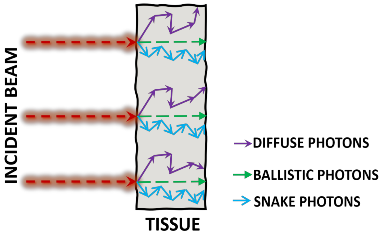
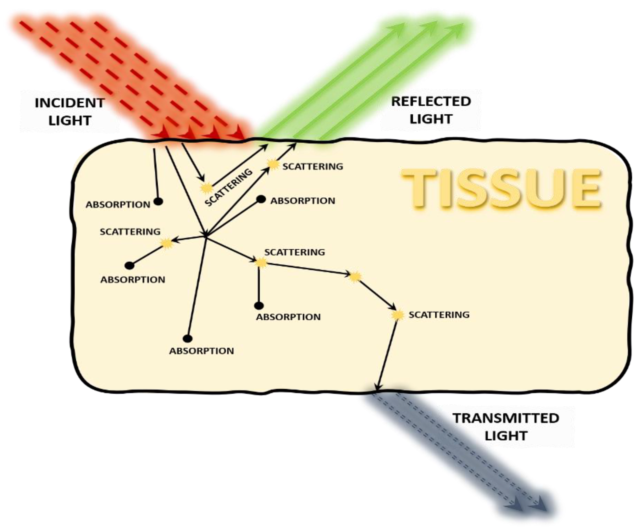
2. Photon Propagation through Tissue

When light interacts with diffusive matter such as tissue, it is scattered and attenuated. Propagation of the light through tissue is mainly determined by two parameters, an absorption parameter μ_a and a scattering parameter μ_s. The absorption parameter describes reduced photon survival rate through the medium and is defined as the probability of absorption per unit length. Absorption events are random processes and are caused by spontaneous quantum interactions between the biological molecules and the light photons. On absorption of a photon, the electron in the absorbing molecule is elevated from the ground state to an excited state, and after a characteristic time called the lifetime, the electron returns to the ground state. While returning to the ground state, the electron can produce heat or generate another photon in a randomized direction. This is referred to as fluorescence, where the initial and final photons can have the same or different wavelengths. The scattering parameter describes alteration of the photon paths in the medium and is defined as the probability of photon scattering event per unit length. A scattering event is an interaction between the photon and the surrounding molecules, resulting in a photon’s direction change without an absorption-emission cycle. The scattering coefficient has a characteristic value of about 10 cm⁻¹, and it is considerably more significant than the absorption coefficient for most biological tissues. Consequently, a photon experiences many scattering events until it is absorbed. Since photons scatter in random directions, the photon trajectory resembles a random walk, resulting in a diffusion-like behavior. This behavior is illustrated in Figure 1.

For biological tissues, the scattering of each photon is in the forward direction with high probability, but a random direction is obtained due to the diversity of scattering events. The effect of multiple scattering is expressed with the aid of an anisotropy factor g, which defines the degree of forward-scattering, and gives the reduced scattering coefficient μ_s′ = μ_s (1 − g). The anisotropy factor g is known for different types of tissues. It varies from −1 to +1, where g = 1 corresponds to forward scattering, g = −1 corresponds to backward, and g = 0 stands for isotropic scattering. Typical values of g for soft tissues lie between 0.80 and 0.95 [4]. This anisotropy factor is the mean cosine of all scattering angles and is defined as

$$g=\langle \cos \theta \rangle ={{\displaystyle \int }}_0^{\pi }\cos \theta p\left(\theta \right)2\pi \sin \theta d\theta$$

(1)

where p(θ) is the probability density function describing the anisotropy of the medium.

Biological tissues are complex since scattering is caused by a mixture of particles of different sizes and characteristics. A valuable approximation for considering the anisotropy in tissue is the Henyey–Greenstein phase function [20].

$$p\left(\theta \right)=\frac{1-g^2}{{\left(1+g^2-2g\cos \theta \right)}^{\raisebox{1ex}{$3$}\!\left/ \!\raisebox{-1ex}{$2$}\right.}}$$

(2)

Photons passing through tissue are classified into three types, as shown in Figure 2: ballistic photons, whose original direction is unchanged; snake photons that are slightly scattered from the propagation axis but maintain some coherence; and diffusive photons where all coherence is lost. A medium of thickness L is considered highly diffusive when the transport mean free path l = 1/μ_s′ << L. For biological tissues, the mean free path is about 0.1 cm. Photon propagation through the tissue can be described either by analytical theory or transport theory [21]. The analytical theory uses Maxwell’s equation and considers the wave nature of light. The complexity of biological tissue makes it extremely difficult to use Maxwell’s equation for computation. Therefore, transport theory is used to study the propagation of photons in thick biological tissues. Transport theory is based on photon particle flow within the medium and is governed by the radiative transport equation (RTE). The RTE is derived using the conservation law for the light intensity or energy radiance, defined as the energy flow at position r and time t per unit time per unit area through the unit solid angle. The complete RTE is an accurate description of light propagation through tissue but has an analytical solution only in a limited number of scenarios. Therefore, an approximation is used, called the diffusion approximation, an expansion of the RTE in first-order spherical harmonics. The assumption is that the reduced scattering coefficient is much larger than the absorption coefficient. In this approximation, the radiance is expressed as a weighted sum of the photon fluence rate, which is the integral of the radiance over the entire solid angle, and the current density, defined as the net energy flow per unit area per unit time. After several mathematical manipulations [22], the RTE can be simplified and rewritten in the diffusion form:

$$\frac{\partial \varphi \left(r,t\right)}{c\partial t}+{\mu }_a\varphi \left(r,t\right)-\nabla .\left[D\nabla \varphi \left(r,t\right)\right]=S\left(r,t\right)$$

(3)

where $D$ is the diffusion term defined as $D=1/3\left({\mu }_s^{\prime }+{\mu }_a\right)$ and $S\left(r,t\right)$ is the source term assumed to be isotropic.

Another approach uses Monte-Carlo (MC) methods. Monte-Carlo methods, like most other light transport methods, simulate the scattering and absorption of photons in any given medium. At this moment, MC methods are the only type of algorithms for simulation light propagation in tissues that are able to accommodate a wide range of light sources and geometries. MC methods provide a virtual, near-realistic picture of real-world light propagation processes [23]. The MC method for light propagation starts with a pencil beam which is perpendicularly incident on a multi-layered medium. Since pencil beams have infinitely small widths, the MC method calculates the medium’s impulse response or Green’s function. First, a photon packet with an assigned initial weight is launched into the sample. Then, the current step size of the packet is calculated. If the photon packet is about to hit a boundary, a fraction of the packet weight will be transmitted and reflected according to Snell’s law and Fresnel’s equations [24]. Following this, the photon packet is moved, absorbed, and scattered, propagating through the sample until it reaches either the upper or lower boundary and its properties are registered. Once enough photon trajectories are computed, the collective distribution of all photons will provide a reasonable estimate of the proper solution to the transport equation, and many physical properties can be estimated. The MC method has many improvements that incorporate other interaction types such as fluorescence and Raman scattering [25], time and frequency-resolved setups, and extensions to 3D samples [26,27,28]. More recently, MC methods have also found applications in the food industry [29], deep learning [30], to study chemical processes [31], and mainly in biomedicine. Many available Monte-Carlo-based tools are online [11,31,32], customized for light propagation in biological tissues to help the biomedical community access efficient and accurate modeling of light transport.

The human body has four basic types of tissue: connective tissue, epithelial tissue (skin, linings of various passages inside the body), muscle tissue, and nervous tissue, with these containing subcategories, for example, skeletal muscle, smooth muscle, and cardiac muscle. Their optical properties cannot be outlined here due to lack of space. For a brief example, skin structures and the underlying tissue that absorb photons are called chromophores [32,33,34]. Different chromophores have scattering and absorption coefficients that are very much dependent on wavelength and thus affect attenuation. For example, common skin chromophores include hemoglobin, melanin, water, and inhomogeneous factors such as tattoos. This wavelength dependency is used to create light-based therapy procedures, design optical devices, and analyze optical spectra and pictures for diagnostic purposes [35,36].

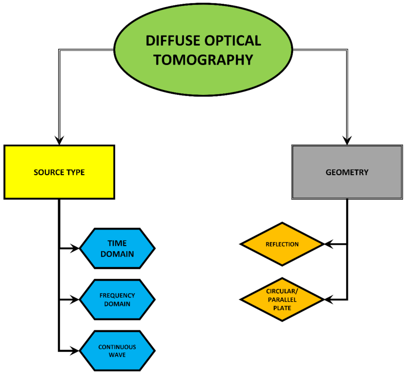
3. Diffuse Optical Tomography (DOT)

Having seen the various optical properties of tissues and light-tissue interactions, we now move on to the subject of imaging tissues using diffuse light. Diffuse optical tomography (DOT) is an imaging technique that uses diffuse light to image soft tissues, with applications ranging from the functional imaging of the brain [37,38,39], and breast cancer research [40,41], to name a few. Due to the nature of light sources used and the type of photons used for imaging, DOT is considered one of the best state-of-the-art technologies for deep tissue imaging. This is due to the fact that DOT is able to break the conventional barrier by imaging deep within the tissue (>10–15 mean free path lengths) [42]. In fact, the first clinical trial using optical light was conducted in ACRIN 6691, where the diffuse optical spectroscopic imaging (DOSI) was used to predict the clinical outcome in breast cancer patients undergoing neoadjuvant chemotherapy (NAC) [40]. As a multidisciplinary technology, the imaging capabilities of DOT combined with signal processing and computer vision allow us to obtain millimeter resolution and reasonably high penetration depth [6,42,43]. However, the path taken by diffuse photons within a tissue is unknown, and hence imaging with such diffuse photons requires inverse problems to be solved for image reconstruction [44,45,46,47,48]. Based on these source types, DOT can be categorized as time-domain (TD), frequency-domain (FD), or continuous wave (CW) systems. Another classification is based on measurement geometry: parallel plate and circular arrangement. Figure 3 shows the different types of diffuse optical tomography systems.

In the CW system, a laser of constant intensity or modulated at low frequency (a few kHz) is used to sample the tissue. The attenuation of the signal propagating through the tissue is measured to determine the tissue’s optical properties. It is relatively easy to implement and faster, but a single measurement cannot differentiate the tissue absorption and scattering coefficient [49,50,51,52]. A CW system gives the least information per source-detector pair. Within the diffusion approximation, a tissue is described by space and time-dependent absorption, scattering coefficient, and refraction index [22,53,54,55]. At least three independent measurements are necessary in order to separate these properties at a single wavelength measurement.

A simple simulation of imaging a compressed breast in a parallel plate geometry is shown in Figure 4. In this simulation, a compressed breast is modeled as an oblate spheroid with a polar radius of 20 mm and an equatorial radius of 22 mm. A small sphere with a radius of 2 mm is placed in the center of the oblate spheroid and is given the optical properties of oxy-hemoglobin. This serves as a test object. The homogeneous breast tissue and the test object (oxy-hemoglobin sphere) are given optical properties according to references [35,36]. The oblate spheroid is placed inside a glass box, and simulated output data are taken from two parallel sides, as shown in Figure 4B. Two billion photons are used in the Monte-Carlo simulations using the ValoMC toolkit [56]. The output light is then normalized and adjusted according to the source term, and the resultant output is averaged out for all the angles. Then, an inverse problem [56] is applied to obtain the general shape and location of the inhomogeneity.

FD systems employ an intensity-modulated laser source (a few MHz–1 GHz) to irradiate the tissue and detect the amplitude and phase of diffusing waves [7,57,58,59,60,61,62,63,64,65,66]. FD systems contain more information than CW systems [22,53,67]. The additional information from the phase makes it possible to simultaneously determine the absorption and scattering coefficient in a single measurement. The detection can be either homodyne or heterodyne. FD systems are more complex than CW systems. A hybrid system employing both the CW and FD systems has been designed for optical tomography that employs a limited number of FD measurements and a larger CW measurement set [68].

In TD systems, an ultra-short laser pulse irradiates the tissue. The short laser pulse passes through the tissue and spreads in time due to scattering, which deviates the photons’ path within the media. Photons take a much longer path causing a temporal shift and broadening of pulse [69,70,71,72,73]. The detection electronics are based on photon counting at a particular point of the sample with sensitivity at a single-photon level. This temporal behavior of exiting photons is referred to as the temporal point spread function (TPSF). The diffuse photons that travel more distance in the tissue arrive later and contain information about the absorption coefficient. TD systems have the highest amount of data per source-detector pair but are the most complex and costly.

The DOT system can be employed in two different geometries based on source-detector position: reflectance and transmittance geometry [74,75,76,77]. In reflectance geometry, the source and the detector are placed on the same side of the sample, while in transmittance geometry, they are on the opposite side of the sample. The time-domain diffuse optical tomography system has been developed by many academic groups [43,78,79,80,81,82,83].

4. Inverse Problems in DOT

As explained above, in DOT, the medium’s optical properties and the spatial distribution of the optical properties are reconstructed from the measured signals. The scarcity of ballistic photons and the loss of imaging information from multiple scattering events result in a non-linear ill-posed inverse problem [84], and appropriate solutions must be applied to solve this challenging task. DOT reconstruction problems are part of a broader class of tasks called inverse problems [85] which has a general form written as follows:

$$Find x\in X from data y=A\left(x\right) + \delta , y\in Y$$

(4)

where $X$ is the optical parameters space, $Y$ is the measurements space, $A$ is the propagation model of photons convolved with the optical component response, and $\delta$ is the noise mechanism in the system. The traditional technique to solve this problem uses an analytical iterative-based algorithm [84]. This method consists of several steps: First, the time-resolved signals are registered. Then, the forward problem is calculated using a forward model, noise model, and guessed optical properties. The forward problem result is compared to the measured signal, and iteratively the guess is modified to achieve perfect agreement with the measured data. Furthermore, analytical reconstruction algorithms possess an additional term other than the data-fit term, called the regularization term. Its goal is penalizing “bad” non-physical solutions which cannot represent the proper solution we search for in the optimization process.

Since most reconstruction algorithms are ill-posed in nature, the regularization terms are crucial for attaining good results since they minimize the space of all possible solutions into only a subset of physically accurate ones. Hence, analytical algorithms have two separate mechanisms which encapsulate our understanding of the underlying physics and the attributes of the solution space to help guide the optimization process in the right direction. However, despite its many advantages, analytical methods suffer from very high computational cost, and in the context of DOT, from an inability to achieve accurate results for realistic 3D problems. Therefore, it has become customary to employ deep learning tools to solve reconstruction problems [6,9,81,86,87]. In the case of diffusive imaging, this refers to the mapping between the optical properties of the media to the measured time-resolved signal registered by the detectors. Typically, forward mapping uses a relatively simple model to make the reconstruction process computationally feasible. This leads in many cases to an oversimplified model that cannot reproduce the realistic properties of the physical process it aims to describe. This does not happen in the deep learning approach since the learning part minimizes the error on training data pairs. The forward model does not have to be understood, and the minimization process can indirectly learn the inverse mapping. If the training process is done correctly and sufficient data are available, the inverse mapping learned by the network can incorporate many of the complex processes which analytical models tend to neglect.

Despite this, deep learning techniques suffer from several drawbacks as well. The need for a large dataset when training a network and the relatively high effort linked to acquiring real data leads in many cases to use simulated data for large portions of the training process. Since the simulated data do not perfectly emulate realistic conditions, this can lead to a big performance gap when transitioning to real data training and testing. Additionally, deep learning methods use the data and the data alone to formulate their solution, and this is its best and worst attribute. This is beneficial since it is applicable for almost any task for which enough training data are available. However, since the deep learning network acts as a black box, it has no prior knowledge of the physical process it tries to solve. Therefore, deep learning methods need to understand the space of correct solutions and understand the underlying physics of the problem. This is a highly demanding task, and when an insufficient amount of data are available, it can be almost impossible to solve. The scarcity of data in biomedical applications leads directly to this problem. Thus, increased effort is made towards incorporating methodologies and prior knowledge from analytical methods into the deep learning schemes to help reduce the complexity and computational burden of the problem. Deep learning offers a powerful and versatile toolkit that can be utilized for many problems and in numerous constellations. In the next sections, the concept of deep learning will be introduced, and a detailed review of the applications of deep learning for solving DOT inverse problems is conducted.

5. Deep Learning

In recent years, the subject of machine learning (ML), with an emphasis on deep learning (DL), has given rise to the most widely used algorithms in artificial intelligence. DL is a form of a model with multiple learning layers [88,89]. These models are called artificial neural networks (ANNs). The idea for these models is influenced by information analysis in many living beings, based on the communication between brain cells [89,90]. Each layer of an ANN contains units called artificial neurons. Each neuron has a real number that describes the neuron’s state. The neuron can transmit a signal through connections called edges to neurons in the next layer.

The signals coming out of the neurons are also real numbers. Each neuron’s state is determined by the output of a non-linear function (activation function) on the sum of the incoming signals. Usually, each edge contains a weight that determines the strength of the connection between the two neurons. These weights are defined as a learning parameter because the weight values are updated during the training process. Another learning parameter is bias. Each neuron contains a bias whose function is to balance the incoming signals. As noted above, the neuron’s state is determined by the activation function’s result on the weighted signals’ sum. Usually, the bias is added to each amount to balance the amount of the weighted signals. Like the weights, the bias is updated during the learning process. The network layers are divided into input, output, and intermediate (hidden) layers [88,89,90]. The input layer contains the information that the network needs to analyze. In the output layer, the result of the calculation of the network is obtained. The hidden layers connect the input layer to the output layer and are intended to extract features from the incoming information. DL refers to ANN networks having several hidden layers, where there are different architectures for these networks such as deep neural network (DNN), convolutional neural network (CNN), deep belief network (DBN), and recurrent neural network (RNN) [88,89,90,91,92]. The networks can also be classified based on the learning processes such as supervised, unsupervised, and semi-supervised [88,89,90,93].

Although heavily used in recent years, the idea of ANN is not new and was first proposed in 1943 by Warren McCulloch and Walter Pitts [94]. In 1958 Frank Rosenblatt developed and introduced a basic neural network method called the Perceptron algorithms with an input and output layer (also called single-layer Perceptron), which had many similarities to the proposal by McCulloch and Pitts [94,95]. At first, this method seemed to show promise; however, in 1969, Marvin Minsky and Seymour Papert showed that this method is limited and showed that perceptron could not learn XOR operation [96]. They argued that the Perceptron model needs more learning layers to learn more complex problems, which is not possible in the algorithm’s learning process, which led to the freezing of the domain of the ANNs until the mid-1980s [97]. Instead, the backpropagation process solved the solution, an algorithm with ancestors as early as the 1960s. Only in 1986 did researchers first introduce the use of this algorithm for the learning process of ANNs, which forms the basis of today’s ANN networks [98]. From there, the field of ANNs evolved, and networks began to solve complex problems like the identification of shapes and letters [99,100].

The learning process of ANNs requires memory and processing power, and the more complex the network, the greater the need for these resources. Besides, more extensive data were needed for the learning process. That is why the field leaped forward in the last decade [89,91]. The availability of graphics processing units (GPUs) at a cheaper cost and the advantages of GPU over CPU has resulted in the neural networks becoming deeper and more powerful. Researchers have discovered new activation functions that are more effective, and regularization techniques that streamline training have been developed during this time. All of these have made the field of DL state-of-the-art machine learning techniques [101].

Today, DL algorithms are applied in various fields such as computer vision, voice, language analysis, signal processing, bioinformatics, drug design, and more [88,89,91,101,102,103]. In recent years, researchers working in medical image analysis investigated the use of DL algorithms differently. Many studies have been written on computer vision architectures to analyze information from medical examinations such as blood tests, X-rays, ultrasound, and magnetic resonance imaging (MRI) [103,104]. The networks learn to perform different tasks: detecting tumors, classifying cells, and detecting various diseases. Today, these networks’ accuracy is extremely high, and their ability to analyze is swift and surpasses human ability. Another example is the use of networks to recover information coming from imaging systems to obtain medical information. The use of networks has given rise to new imaging methods and streamlining of existing imaging methods [105,106,107,108].

6. Deep Learning Diffuse Optical Tomography

Recently deep learning algorithms have been increasingly used to solve diffuse optical tomography problems for biomedical imaging. In recent works [10,43], it has been shown that using convoluted neural networks to estimate bulk optical properties and imaging is more accurate and faster compared to other existing methods, thus showing us a way forward to use convolution neural networks (CNN) along with optical tomography techniques.

One of the preliminary works in this field was submitted to the European Conference on Biomedical Optics conference to be held in June 2021 [109], titled “Anomaly Detection Inside Diffuse Media using Deep Learning Algorithm”. In this paper, a simple, densely connected neural network with only one hidden layer was used to reconstruct 2D spherical objects with embedded spherical occlusions. A total of 16 sources and 16 detectors were uniformly arranged along the circumference of the phantom.

Therefore, the input to the network was the time-integrated flux of each detector from each source totaling 240 (16 × 15) values. The network output is trained to regress to the absorption coefficients of each location in the phantom. A significant improvement of up to 77% compared to the Tikhonov regularization method was registered, thus, showing the utility of this approach. Another interesting paper [9] used simulation data generated using the Toast++ toolbox [11] of 2D breast-shaped objects with asymmetrical embedded anomalies. Two sources and 128 detectors were placed to detect backscattered light from the sample, and the network was trained to reconstruct the spatial distribution of the sample’s optical properties. The network comprises an initial dense layer (generalize the filtered-back-projection operator) followed by multiple convolution layers with various channel numbers and kernel sizes. A comparison to an analytical approach was made, and higher accuracy with considerably lower inference time was attained. Moreover, a follow-up paper [82] applied an additional loss and transfer learning procedure, and an additional improvement was registered. The entrance of time-resolved DOT was introduced in [9], where a time-resolved RTE-based solver was used to simulate the data. The time-resolved data registered in different detectors were used to detect cancerous cells. This was effective even though the detection was accomplished by classifying predefined locations as containing tumors instead of regressing to their continuous location. High accuracy was achieved for time-resolved data even when noise sources were introduced. In another paper yet to be published, time-resolved measurements were used to reconstruct anomalies embedded inside 3D scattering media. The objects were spherical anomalies with various sizes and locations embedded inside a 5 cm diameter sphere. To emulate realistic conditions, the optical properties of the anomaly and surrounding tissues were taken from available breast tissue experimental data. The network was trained using a large, simulated dataset of time-resolved measurements generated using the Toast++ toolbox [110]. Figure 5 presents an example of the objects and the optical devices. Two sources and three detectors were used. The time-resolved measurements registered in each detector are also shown.

2D convolution layers followed by three fully connected layers were used to regress to the Cartesian coordinates and size of the embedded anomaly. The best-performing model detected the anomalies with high accuracy and proved that good results could be attained using a small set of optical measurements. In another article [17], the propagation of angled light sources in compressed breast tissues with sub-surface inhomogeneities and the use of novel inverse problems in combination with deep learning methods were studied. The U-Net deep learning algorithm was constructed to detect and reconstruct test objects with a radius of 1 mm with high resolution at a penetration depth of up to 4 cm with a minimal error of 0.0334 mm in terms of mean squared error (MSE). Despite their relative success, the presented algorithm still fails to implement our physical knowledge of the problem. This tremendously enhances the complexity of the task since the network is treated as a black box, and it has no prior knowledge of the problem. In an interesting article [111], a new approach that exploits prior information was introduced. By performing a perturbative analysis of the forward mapping between the scattering field and the boundary measurements, they proved it can be reduced to a family of 1D convolutions in polar coordinates. Motivated by this understanding and using the filtered-back-projection method [112], the inverse mapping can also be represented by the convolutions layer with a specific structure. The use of physical knowledge guided the architecture design, and they showed that by using their method, both the forward and inverse mapping could be accurately represented by neural networks. Deep learning and DOT are still in their juvenile form. Most implementation of this combination was performed using basic tools and in simplified cases. The next step will be utilizing the knowledge acquired in other fields focusing on inverse problem-solving. The following section will be dedicated to reviewing the recent trends of this approach to inspire further advances in deep learning-based diffuse imaging.

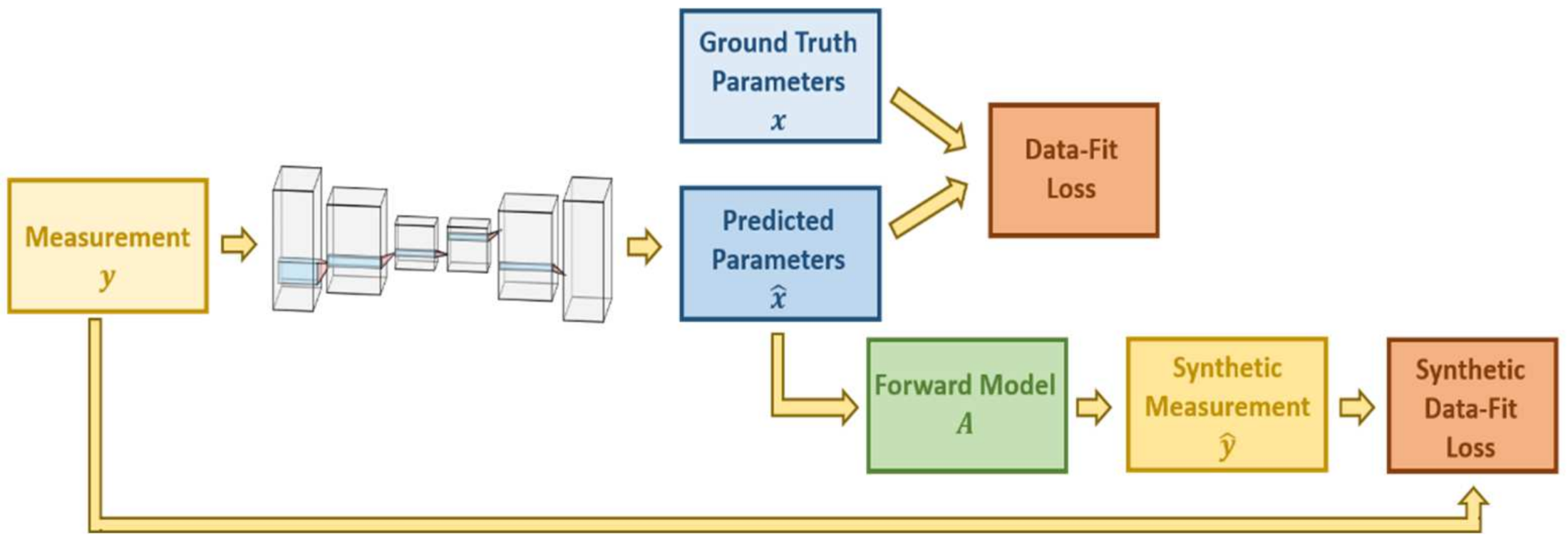
7. Deep Learning as a Tool to Solve Inverse Problems

Having looked at the basics of deep learning, we will now review the recent trends and tools used by the inverse problem community and explore the relevant mechanisms which are used to achieve enhanced performance for those tasks. Deep learning techniques used for inverse problem solving can be broadly classified into two distinct types. The first type is feed-forward networks, in which the network is employed in a traditional direct manner with training pairs used to optimize the network parameters. The second type is regularization networks, inspired by the regularization terms, more commonly found in analytical methods. In the following section, we will present these two distinct methods and describe how they are implemented.

7.1. Feed-Forward Networks

Feed-forward networks are the archetypal models used in deep learning. These networks have a simple form where input data are fed to the network and output data are generated. However, despite its relatively simple architecture, it has led to numerous successes [113] for prediction models with big data and improvements in various fields including one of its variants, the CNN, which is considered the leading technique used in computer vision and in many other fields [114].

Although feed-forward networks are based only on training pairs, numerous strategies are employed to help exploit the network abilities and enhance the reconstruction performance. One popular approach is using the network in a two-phase manner. The first phase uses some form of initial mapping to help reduce the complexity of the network task, and the second phase consists of training the network by minimizing an error term and optimizing the network parameters. As explained above, reconstruction problems are typically ill-posed. Therefore, one way to meaningfully map the input is using the training data to establish a low-dimensional representation of the measurement space and transform the problem to be well-posed. It is customary in computerized image reconstruction tasks to discretize both the parameters and measurements into finite elements. Consequently, both can be identified using a column vector:

$$x={\left(x_1,\dots ,x_n\right)}^T\in R^n, y={\left(y_1,\dots ,y_m\right)}^T\in R^m$$

(5)

where n is commonly much more significant than m, as in most DOT setups. Hence, to transform the problem to be well-posed, a $k$ dimensional latent space representation of the parameter space is needed, where$k\le m$. This can be made using an autoencoder [115,116] or its successor, the variational-autoencoder [117,118,119]. After the representation is found, the task can be reformulated by reconstructing only the latent representation $\tilde{x}$ from y, then, using the decoder part, the original $x$ is generated, this is shown in Figure 6. In [120], this scheme was implemented for lung electrical impedance tomography, and a significant improvement over previous methods was registered.

Another type of strategy which uses two-step reconstruction is possible. This method incorporates prior physical knowledge by first using an inversion of a simplified propagation model (pseudo-inverse) $\widetilde{A^{-1}}$ to map from the measurement space to the parameter space. Then, a network is trained to reconstruct the actual parameters from the simple initial guess generated in the first step. The two steps reconstruction can be written as follows:

$$\begin{gathered} x={\mathsf{\Psi }}_{inverse}\left(y\right), {\mathsf{\Psi }}_{inverse}={\mathsf{\Phi }}_{NN}°\widetilde{A^{-1}}, \\ \widetilde{A^{-1}:}Y\to X, {\mathsf{\Phi }}_{NN}:X\to X \end{gathered}$$

(6)

These algorithms rely on the fact that by mapping the input to a physically possible solution and the same space as the desired solution, the computational burden is reduced. Furthermore, instead of directly reconstructing based on the estimated inverse, the network output can be residually connected to the estimate. Hence, the network goal will be to refine the initial guess. This method was used in many biomedical imaging fields, such as computed tomography [121,122], compressive sensing [123,124,125] and MR imaging [126], and is represented in Figure 7.

So far, our physical understanding of the problem was only implemented indirectly. The knowledge of the forward model $A$ or its approximate can be utilized along with a neural network in a self-consistent manner. In [127], a self-consistent network was implemented for geo-steering inversion. The architecture is as follows. First, the observed measurements $y$ are passed through a neural network to generate the predicted parameters $\widehat{x}$. Next, the network output is compared to the ground truth parameters and passed into a forward model $A$ to generate synthetic measurements $\widehat{y}$. The synthetic measurements are compared to the real measurements and a combined loss of both comparisons is calculated; the network is trained to minimize both losses. The addition of the synthetic simulation part can be seen as a form of regularization, similar to the self-consistent loss found in Cycle-GAN [128]. The network is constrained to output realistic solutions since they are used to regenerate the original input of the network using realistic physical models. Figure 8 presents this method.

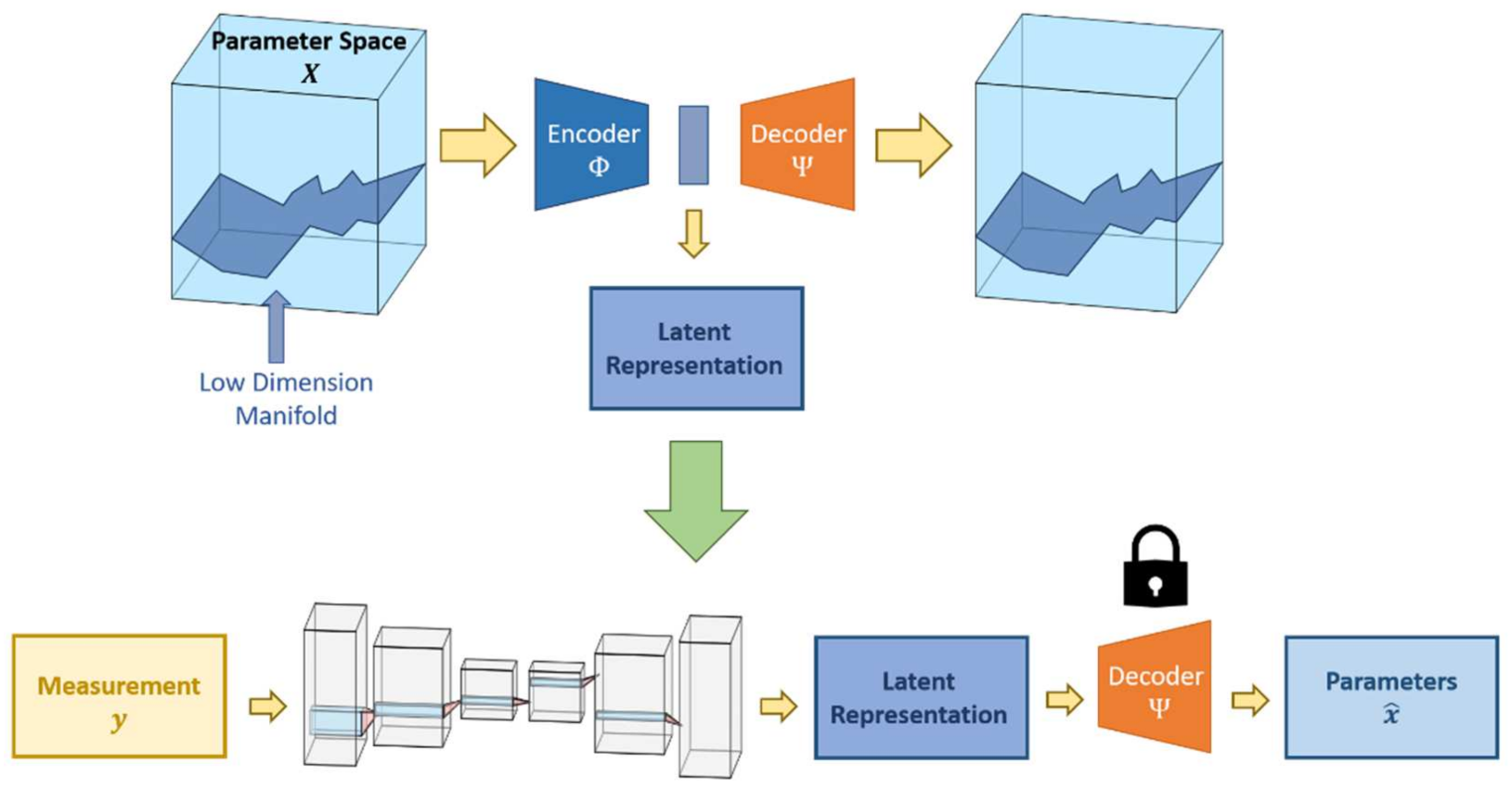
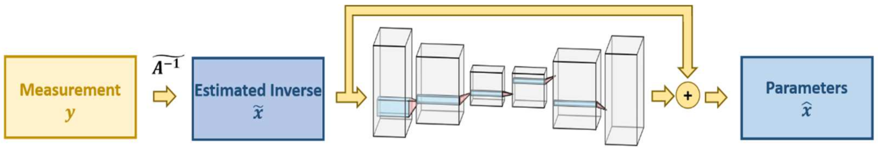
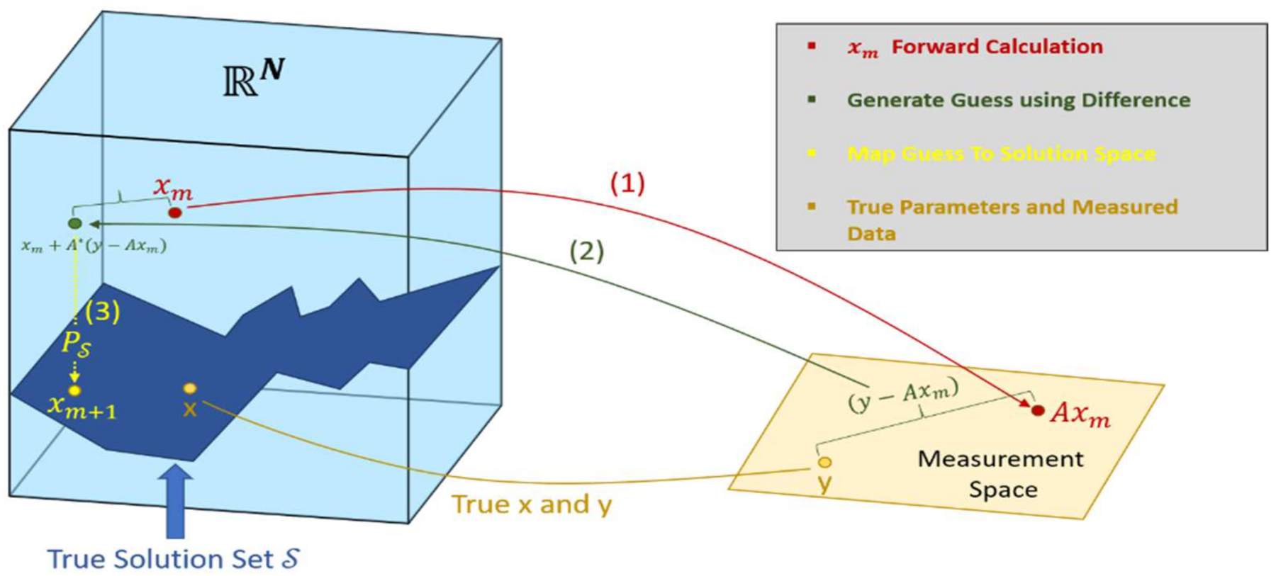
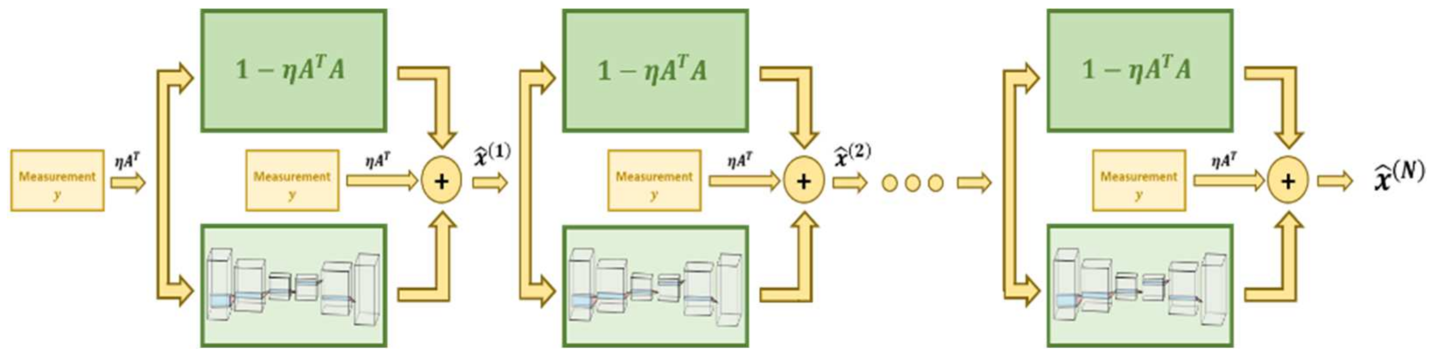
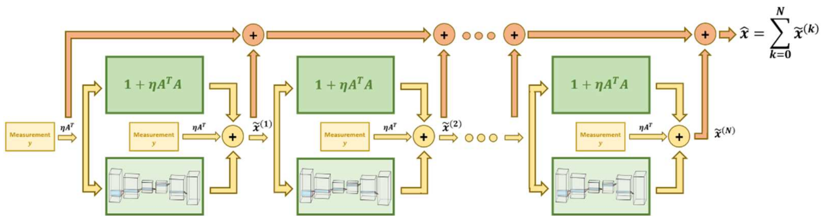
7.2. Regularization Networks

The second class of algorithms focuses on implementing the regularization terms that are crucial to the success of analytical methods. Moreover, regularization networks can typically be implemented as part of an iterative-based optimization scheme. Therefore, both aspects making the analytical approach successful can be utilized using this approach. Up to now, the regularization terms used by analytical methods were based on general attributes of the data like smoothness or sparsity. The idea behind regularization networks is to generate a custom data-specific regularizer based on the available training data. Several common approaches are used in the modern literature. The first approach uses perturbations of the training data in order to train a projector/denoiser that can be implemented later into an analytical algorithm. Suppose that the true solutions $x$ lie on a set $\mathcal{S}\subset {ℝ}^N$, therefore, $P_{\mathcal{S}}$ is a good projector if it satisfies the following:

$$P_{\mathcal{S}}\left(\tilde{x}\right)=x$$

(7)

where $\tilde{x}$ is any perturbed version of $x$ including $x$ itself. Hence, by training the network on a sufficiently diverse and meaningful set of perturbed solutions, the ill-posedness of the problem can be bypassed. After the projector is trained, it can be implemented into a proximal gradient descent algorithm where the trained network replaces the projector. The proposed scheme is illustrated in Figure 9. In [121], this scheme was implemented for sparse-view CT reconstruction. The network was trained using three types of perturbations (identity, linear and non-linear) of the data, and detailed convergence analysis of the algorithm was made.

A different algorithm suggested in [129] used both measurements $y$ and parameters $x$ from the training dataset to train an adversarial regularizer ${\mathsf{\Psi }}_{\mathsf{\theta }}$, the regularizer was later implemented into an optimization algorithm to solve the following problem:

$${\mathrm{argmin}}_{\mathrm{x}}\Vert \mathrm{Ax}-\mathrm{y}{\Vert }_2^2+{\lambda }_1{\mathsf{\Psi }}_{\mathsf{\theta }}\left(\mathrm{x}\right)$$

(8)

The adversarial regularizer ${\mathsf{\Psi }}_{\mathsf{\theta }}$ was constructed as follows. Suppose that the parameters $x\in X$ are drawn from the distribution ${\mathbb{P}}_x$ and the measurements $\mathrm{y}\in \mathrm{Y}$ are drawn from the distribution ${\mathbb{P}}_y$. We define ${\mathbb{P}}_{\tilde{x}}$ as the distribution obtained by mapping ${\mathbb{P}}_y$ using a pseudo-inverse operator $\widetilde{{\mathrm{A}}_{\mathsf{\delta }}^{-1}}$ that incorporates both the contributions of the forward model $A$ and the noise model$\delta$. The adversarial regularizer ${\mathsf{\Psi }}_{\mathsf{\theta }}$ will be trained to discriminate between the two distributions ${\mathbb{P}}_x$ and ${\mathbb{P}}_{\tilde{x}}$. Moreover, we would like the output of the network to be small for $x~{\mathbb{P}}_x$ and large for $\tilde{x}~{\mathbb{P}}_{\tilde{x}}$. This goal can be achieved by training the network to minimize the following loss:

$$E_{X~P_x}\left[{\mathsf{\Psi }}_{\theta }\left(X\right)\right]-E_{\tilde{X}~P_{\tilde{x}}}\left[{\mathsf{\Psi }}_{\mathsf{\theta }}\left(X\right)\right]$$

(9)

Consequently, as proved in the paper, starting from a noisy parameter $\tilde{x}~{\mathbb{P}}_{\tilde{x}}$ and taking a gradient step with size $\eta$ over the regularization network where,

$$g_{\eta }\left(\tilde{x}\right)=\tilde{x}-\eta \cdot {\nabla }_{\tilde{x}}{\mathsf{\Psi }}_{\mathsf{\theta }}\left(\tilde{x}\right)$$

(10)

results in a distribution ${\mathbb{P}}_{\eta }={\left(g_{\eta }\right)}_{\#}{\mathbb{P}}_{\tilde{x}}$ closer to the true parameter distribution ${\mathbb{P}}_x$ in Wasserstein distance [130]. Hence, the regularizer helps in directing our optimization scheme towards reasonable solutions. The available parameters dataset can also be utilized in a different setup to learn a generative prior of the data. To understand this method, let us suppose that the true solutions $x$ lie on a set as was assumed before. A perfect regularizer $r\left(\widehat{x}\right)$ would satisfiy the following:

$$r\left(x\right)=\left\{\begin{array}{c}0 , x\in S \\ \infty , otherwise\end{array}\right.$$

(11)

The optimization problem can be solved by finding a solution for the following task:

$$\widehat{x}=argmi{n}_x\Vert y-Ax{\Vert }_2^2+r\left(x\right)$$

(12)

This method substitutes the perfect regularizer with a generator $G$ that was trained to capture the true distribution ${\mathbb{P}}_x$ by learning to generate a solution that lies on the manifold $\mathcal{S}$ given a noisy input $z\in {ℝ}^K$, $(K<N)$. The subject of learning generative models and approximating high dimensional distributions has been well developed and can be achieved either by using adversarial training for generative adversarial networks (GANs) [131] or with variational-autoencoders [117]. After the generator is trained, the following alternative optimization process is employed to exploit the understanding of the solution space summarized in $G$:

$$\widehat{x}=G\left(\widehat{z}\right) , \widehat{z}=argmi{n}_z\Vert y-AG\left(z\right){\Vert }_2^2$$

(13)

Therefore, we search in lower-dimensional space ${ℝ}^K$ for optimal solutions. Since the generator $G$ is differentiable, the optimization formulated in Equation (10) can be solved using regular gradient-based algorithms. This scheme was developed in compressive sensing [132], and a noticeable improvement over traditional analytical algorithms was registered. However, to the attempt to learn prior information about the solution space also has its weaknesses. The task of learning the full distribution ${\mathbb{P}}_x$ based on the data requires tremendous amount of training samples, and with the low amount of available data, this approach fails to achieve satisfactory results [133]. Consequently, the research community has aimed to develop a method that can combine the strength of the regularization network with the iterative nature and knowledge of the forward operator analytical methods. This process led to the development of unrolled methods. Unrolled optimization schemes are very similar to the projector/denoiser approach suggested above, and the network still plays the role of projecting the temporary solution to the desired solution space $\mathcal{S}$. The main difference is that instead of training the regularization network before the optimization, unrolled methods incorporate the neural network into the optimizer architecture, and the network is trained during the search for the solution.

To understand this method, let us try to solve the same task as formulated by Equation (9) where $r\left(x\right)$ is the perfect regularizer introduced above. The optimization task can be solved using the following update rule for the estimate $\widehat{x}$:

$${\widehat{x}}^{\left(k+1\right)}={\widehat{x}}^{\left(k\right)}+\eta A^T\left(y-A{\widehat{x}}^{\left(k\right)}\right)+\eta \nabla r\left({\widehat{x}}^{\left(k\right)}\right)$$

(14)

Since we do not know what the perfect regularizer is, its derivatives are also unknown to us. Therefore, the idea in unrolled optimization is substituting the $\nabla r$ term with a neural network, which during the optimization will be trained to direct the search towards better solutions. The scheme can easily be presented using block diagrams (Figure 10). This representation shows its recurrent nature and guides us to use recurrent network architectures to implement if efficiently.

Unrolled optimization schemes were implemented for various tasks, such as compressive sensing [134] and MR-imaging [126]. For most tasks, these schemes tend to perform better, especially where the size of the dataset is limited. Moreover, this approach was also extended to other optimization algorithms such as ADMM [135], half-quadratic splitting [136] etc. Despite its comparably good performance for various tasks, unrolling methods suffer from a similar gradients problem as a regular recurrent network. Their structure makes it challenging to train the first layers/iterations since their output needs to be passed through several operations to make an effect. Inspired by their structure, a new method called the Neumann network was suggested [133]. This method estimates the solution to Equation (9) using a Neumann series approximation. Suppose that we know the perfect regularizer $r\left(x\right)$ and it is differentiable, hence, the least squares solution can be written as:

$$\widehat{x}=argmi{n}_x\Vert y-Ax{\Vert }_2^2+r\left(x\right)={(A^{T}A+\nabla r)}^{-1}{A}^{T}y$$

(15)

The inverse operator from Equation (12) can be approximated using the Neumann series expansion [137]. By truncating the series to only $K+1$ terms, Equation (12) can be written in the following form:

$$\widehat{x}\approx {\displaystyle \sum }_{k=0}^K{\left(1-\eta A^{T}A-\eta \nabla r\right)}^k\eta A^{T}y$$

(16)

Like the unrolled method, the gradient operator and the step size can be replaced by a trainable operator and optimized using the training data. This representation can also be presented using a block diagram. This is shown in Figure 11.

In the figure, each block represents another term from the expansion series, it is crucial to notice that the Neumann expansion is only justifiable from a linear operator. However, as shown in the paper, using this approximation is valid for certain assumptions on the distribution and about the operator $\nabla r$. A Neumann network was applied for numerous applications in [133], including compressed sensing, super-resolution, inpainting, etc. For most tasks, it outperformed other competing methods, including unrolled optimization and various other regularizer networks.

The following section describes how to generate breast imaging using standard tools in the field and then all the steps required to reconstruct the image using a deep learning algorithm with actual examples.

8. Tutorial on the Use of Deep Learning for Diffuse Optical Tomography

The previous sections have shown the considerable amount of study conducted in this particular area of research. As can be seen, in order to create a prototype medical system, it is critical to analyze the impact of boundaries and source-detector configurations on breast image reconstruction and classification. These models are mostly evaluated through computer simulations to avoid the costly and wasteful fabrication of clinical prototype systems that might possess intrinsic engineering problems [138]. However, for clinical applications, testing the application and validating it in clinical trials is very critical. Section 3 and Section 6 discuss many imaging geometries and source-detector configurations that exist for imaging tissues. Moreover, many software and algorithms are available to simulate these conditions. The state-of-the-art algorithms include NIRFAST [5], toast++ [110], and ValoMC [56], to name a few. In this particular section, the tutorial is demonstrated using the ValoMC software. For the sake of simplicity and better understanding, a CW system is employed in a parallel plate geometry, and the image reconstruction is demonstrated using a simple U-Net architecture [139]. The details about the optical properties of the tissue, parallel plates, source-detector locations, and the inverse problem are shown in Figure 4 in Section 3. The results are shown using a single 2-D plane. The schematic process for any deep-learning tomography modality is shown in Figure 12.

The operation for deep-learning diffuse optical tomography is as follows:

(1)

Optical property estimation and mesh creation:

To create an accurate tomographic reconstruction, the optical properties of the breast should be known. Typically, in experiments, this is estimated using spectroscopic methods [4,35,36]. However, in simulations, the optical property distributions of the anomalies and the breast tissues are known beforehand. Therefore, the geometry shown in Figure 4 is created using the optical properties in references [138,140].

(2)

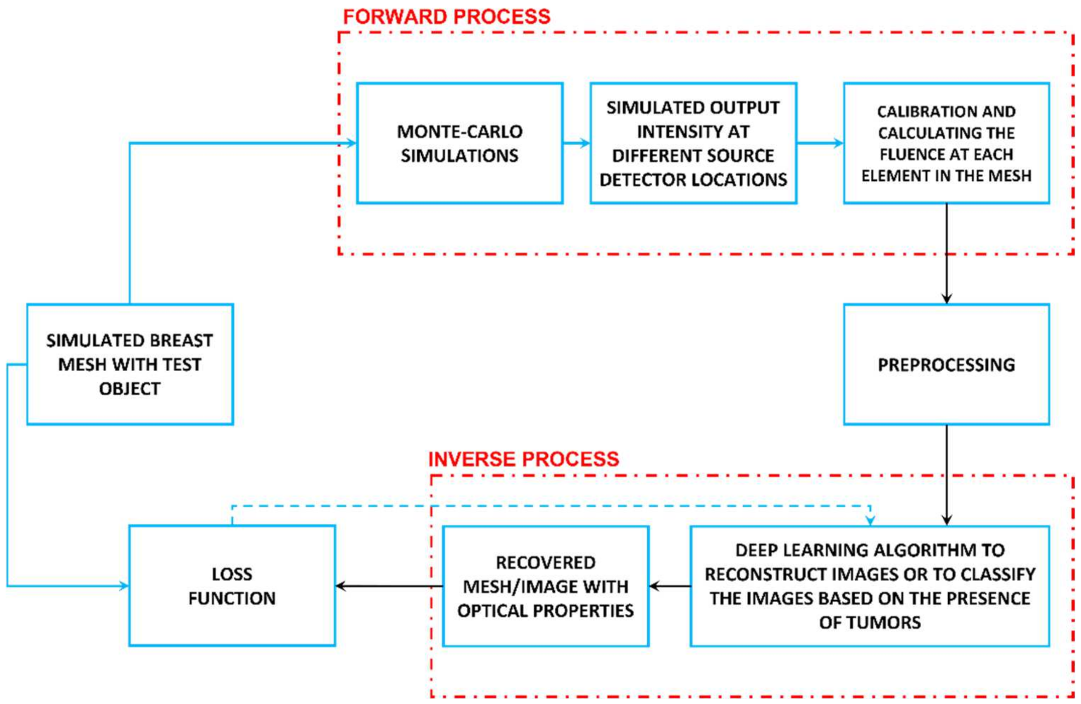
Forward process and data creation:

The light propagation in tissue from the source locations is simulated using a Monte-Carlo algorithm [5,56,110,141,142]. The Monte-Carlo algorithm propagates light through the tissues using the given source and detector locations and collects the output light at the detector.

(3)

Solving the inverse problem and designing the network architecture:

In this step, the data are simulated for different sizes of the anomalies and at different locations, and the simulated output signals are then used to feed the inverse problem to solve DOT. The neural network or deep-learning approach used to solve the inverse problem is highly dependent on the type of datasets used. The various deep learning algorithms and their applications in diffuse optical tomography are already discussed in Section 6.

In the next section, an example which implements all the steps described in this section is shown.

9. Deep-Learning Diffuse Optical Tomography Using Digital Phantoms: An Example

(1)

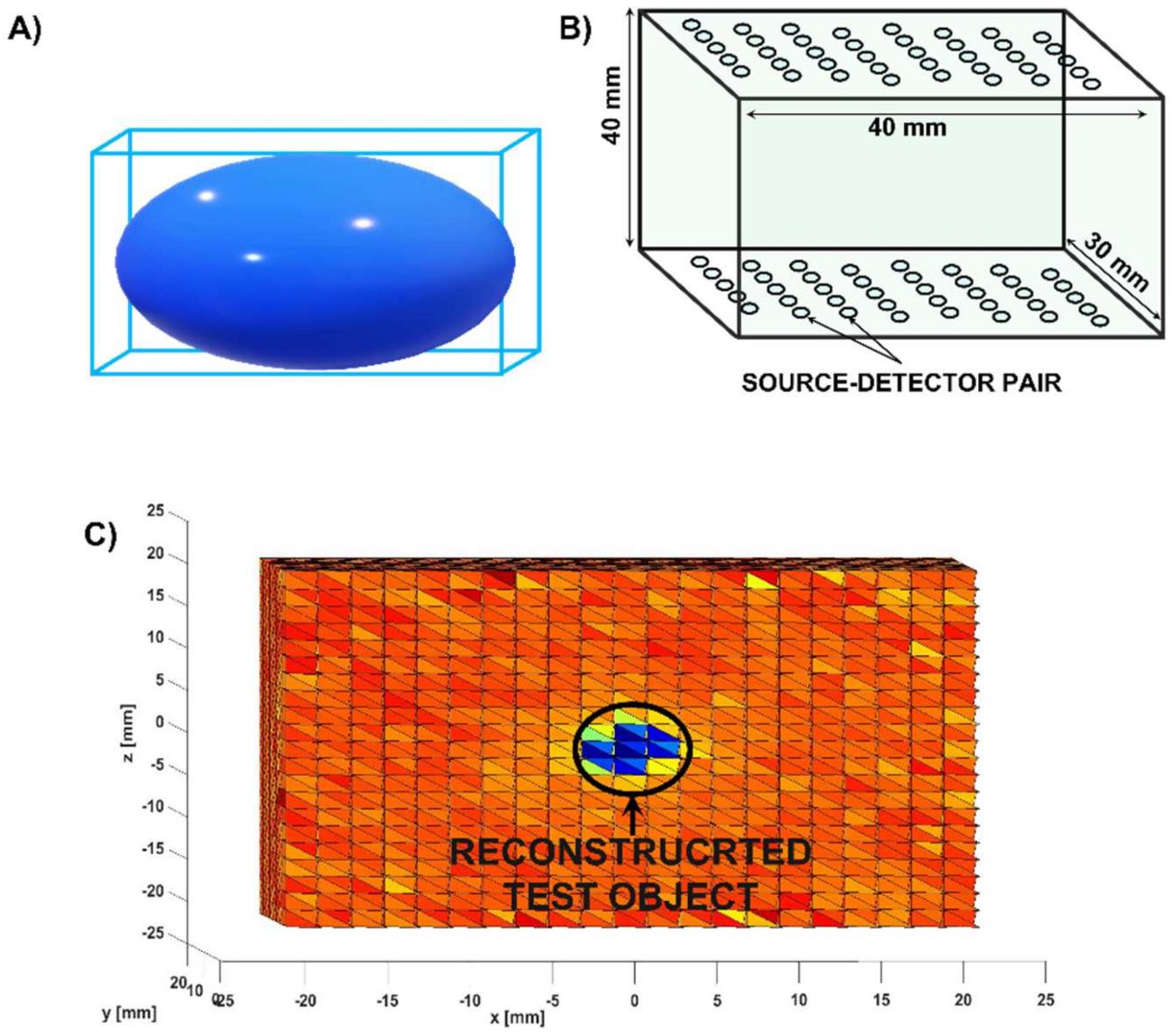
Optical property estimation and mesh creation: Creating the digital breast phantom

The ValoMC program is employed to simulate the geometry and create the mesh. The created mesh and the source-detector locations are shown in Figure 4.

Table 1. Functions to impart optical properties to the medium and fix the source-detector locations.

S. No.	Function	Use	Value
1	vmcmedium.absorption_coefficient	Function used to impart absorption coefficient to the medium.	${\mu }_a$$(\mathrm{glass} \mathrm{box})=0 {\mathrm{mm}}^{-1}$ ${\mu }_a$$(\mathrm{compressed} \mathrm{breast})=0.1 {\mathrm{mm}}^{-1}$ ${\mu }_a$$\left(\mathrm{anomaly}\right)=0.398 {\mathrm{mm}}^{-1}$
2	vmcmedium.scattering_coefficient	Function used to impart scattering coefficient to the medium.	${\mu }_s$$(\mathrm{glass} \mathrm{box})=0 {\mathrm{mm}}^{-1}$ ${\mu }_s$$(\mathrm{compressed} \mathrm{breast})=1.25 {\mathrm{mm}}^{-1}$ ${\mu }_s$$\left(\mathrm{anomaly}\right)=1 {\mathrm{mm}}^{-1}$
3	vmcmedium.refravtive_index	Function used to impart refractive index to the medium.	N (glass box) = 1.013 n (compressed breast) = 1.37 n (anomaly) = 1.4
4	vmcmedium.scattering_anisotropy	Function used to impart scattering anisotropy to the medium.	G (glass box) = 1 g (compressed breast) = 0.9 g (anomaly) = 0.85
5	vmcboundary.lightsource	Define the type of light source and the location of the light source.	Light source and detector locations are set according to Figure 4.
6	vmcboundary.exterior_refractive_index	Define the refractive index of the external medium.	Exterior refractive index is set at 1.5 to create a mismatch between the glass box and surrounding environment.

describes the functions that describe the optical properties of the mesh and how to impart and fix the source-detector locations.

(2)

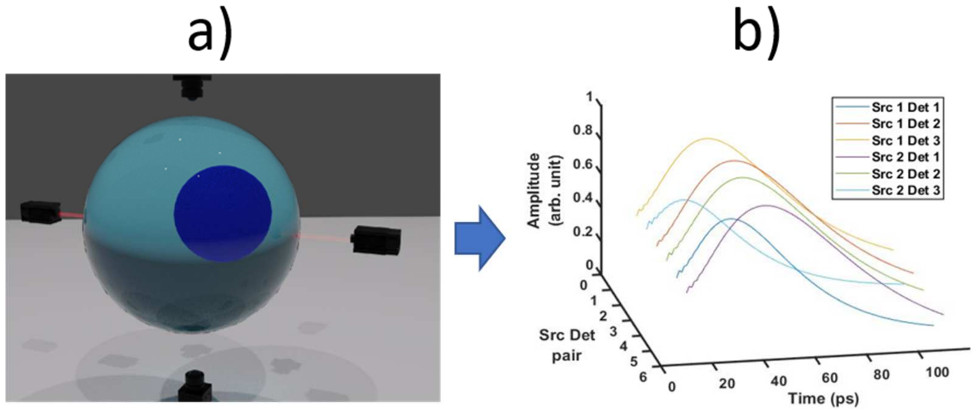
Forward process: Propagation of light through the digital phantom:

As stated above, the ValoMC software is used for this simulation. In this particular study, the anomaly is created as an oxy-hemoglobin sphere of radius 1 mm, and it is placed at 2000 random locations within the compressed breast, thereby creating a dataset of breast images. The forward process is initiated using the function:

solution = ValoMC(vmcmesh, vmcmedium, vmcboundary).

The various parameters that can be calculated using the forward process are shown in

Table 2. Parameter estimation using the ValoMC software.

S. No.	Function	Use
1	Solution.element_fluence	Function that outputs the fluence at each element.
2	Solution.boundary_fluence	Function that outputs the excitance at each boundary element.

. The results of the simulation are shown in Figure 13.

(3)

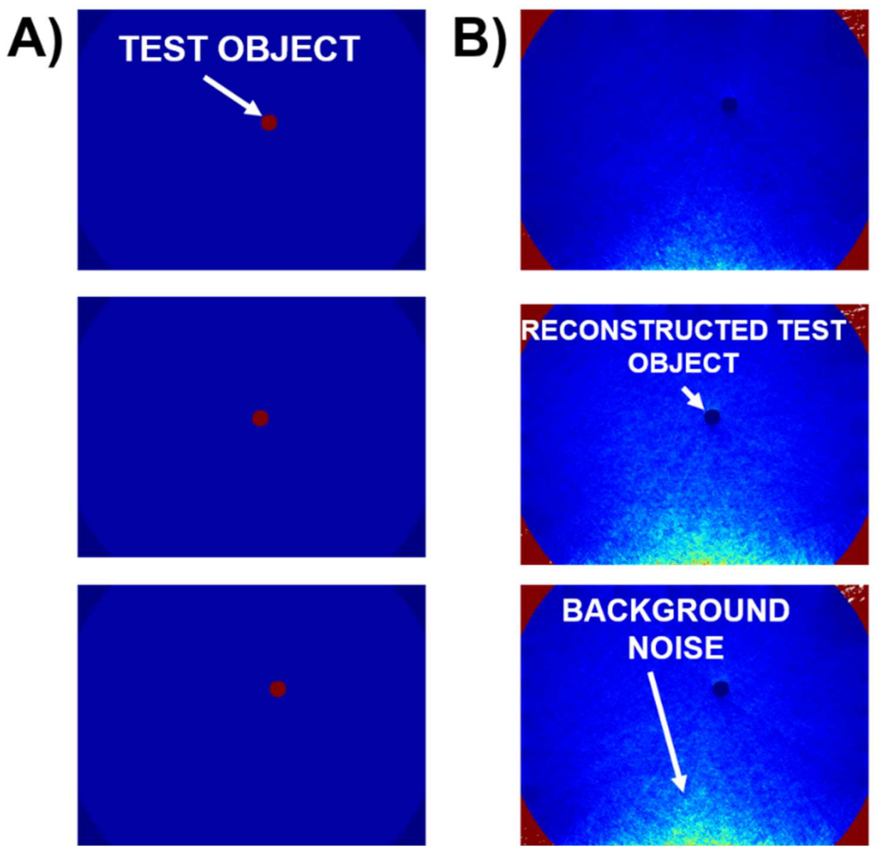
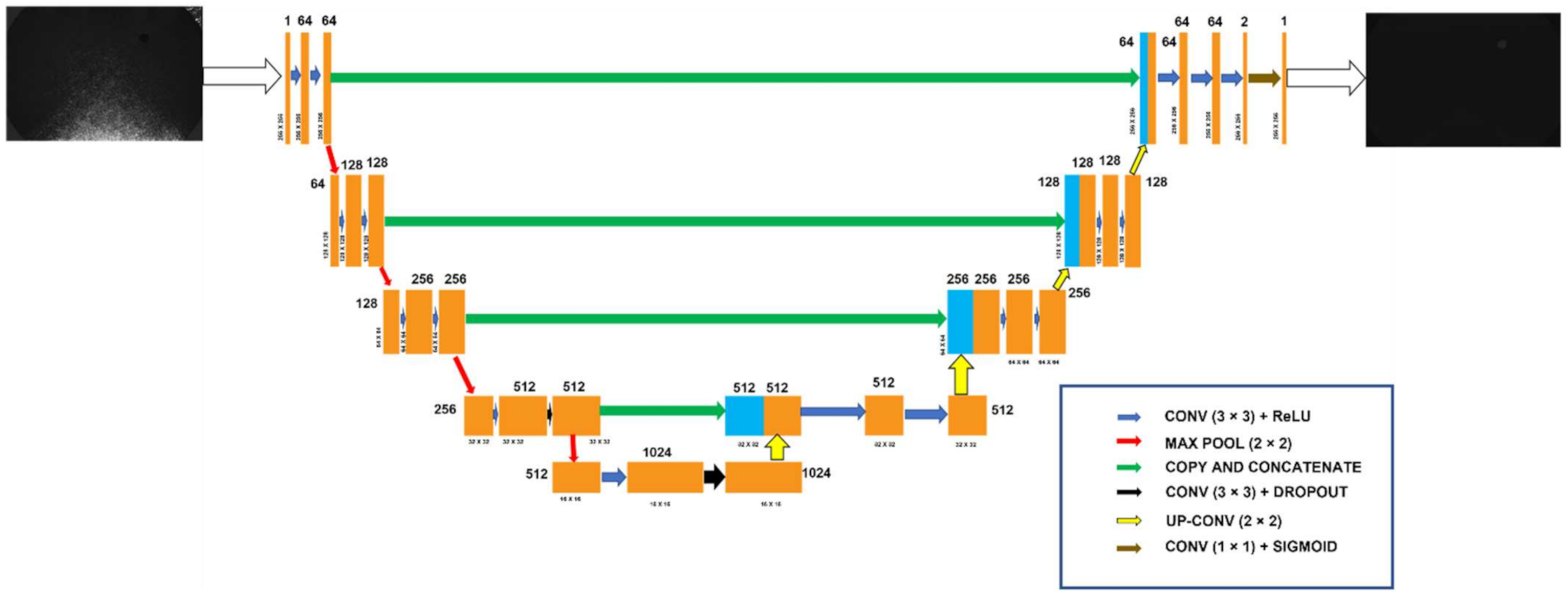
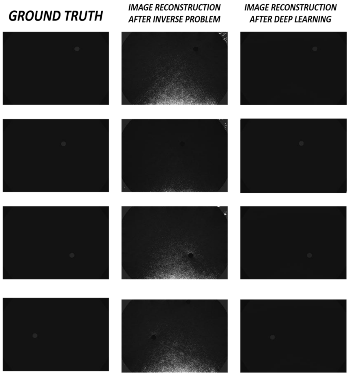
The neural network architecture used for image reconstruction:

This example uses a convolutional neural network (CNN) architecture for image reconstruction [17]. The U-Net network learns from the dataset to detect anomalies in breast tissues produced with the ValoMC program. The network diagram of the neural network architecture is shown in Figure 14.

The CNN design is built on the U-Net architecture’s encoder-decoder concept. First, the images an input layer consisting of 3 × 3 kernels to create an initial feature map. The image is then convoluted and passes through a down sample layer (max-pooling 2 × 2). This process repeats itself four times in the encoder. Following this process, the feature maps enter a batch normalization and ReLU activation layer. After which, they pass through a dropout layer (25% dropout). This feature map then enters an up-convolution layer (transpose convolution 2 × 2). The up-convolution process repeats itself four more times in the decoder to obtain the network output. Skip connections are made with the feature maps obtained at the end of the corresponding stage in the encoder with the feature maps obtained after the up-sample layer to retain the information. The algorithm employs the MSE loss function and runs for 40 epochs. The algorithm learns from the training set, which contains 90% of all the simulated data acquired. With each passing epoch, the algorithm learns more from the data generated. The algorithm is tested with ten percent of the data.

After solving the inverse problem and pre-processing the data, we find that the location of the reconstructed object is fairly accurate. However, it should be considered that the MSE is calculated to by using the intensity of each pixel in the image. Due to background noise and apparent mismatches at the boundary, the MSE of the inverse problem is very low. The difference in contrast between the ground truth and the reconstructed image should also be noticed, where even though the location is reasonably accurate, the optical property reconstruction is not.

On the other hand, such problems do not persist in the deep learning method. The U-Net algorithm can reconstruct the data as close to the ground truth as possible, both in terms of the location and the intensity.

The architecture results are shown below in Figure 15 and compared to the results of the analytical solution. The mean squared error (MSE) loss function is used to check for the performance of the deep learning algorithm, and an excellent result of MSE = 0.0294 ± 0.0012 mm is achieved. The reconstructed images using this method are more explicit and attain a Dice similarity coefficient [143] of 97.98% compared to 48.65% when an analytical solution is used.

10. Conclusions

Diffuse optical tomography is an excellent tool to image irregularities in bulk tissues and investigate changes in the body [4,55,144,145]. It is one of the safest and noninvasive methods available in medical diagnostic imaging [22,53,146]. The different types of geometries used and the source type employed have their advantages and disadvantages. The iterative inverse problems are also cumbersome, time-consuming, and computationally inefficient [6,87,107,120]. Therefore, while employing these methods, one must be accurate and precise to obtain correct diagnostic results. This article reviews different diffuse optical tomography methods and the inverse problems used to solve them. A comprehensive study of deep learning algorithms and their application in solving inverse problems in DOT is also conducted. The literature review shows that deep learning algorithms could prove to be an extremely viable alternative to the ill-posed and computationally inefficient iterative problems [9,86,87]. This is because of the increased efficiency, greater accuracy, and high computational speed of solving inverse problems. The ability of deep learning algorithms to reconstruct images in a noisy environment, work with different types of datasets, their robustness, and the speed of computing makes it an attractive solution to solve inverse problems. However, certain limitations and issues persist in deep learning DOT. Apart from being highly dependent on the dataset and network parameters, the main issue in such research is that it is difficult to train a deep learning network using real-time experimental data because it is near-impossible to collect such a large set of experimental data. Therefore, most deep learning algorithms to solve DOT are trained using simulated datasets, leading to trade-offs in precision and accuracy during real experiments. However, as shown in Section 7.1, Section 7.2, Section 8, and Section 9, end-to-end deep learning algorithms can be applied to solve inverse problems in DOT, and novel imaging techniques and deep learning algorithms can be developed to bring this optical imaging modality closer to real-time experimental procedures. With suitable datasets, accurate data acquisition, optimal loss functions, and the latest architectures, deep learning algorithms, along with advances in diffuse optical imaging systems, could have tremendous applications in the biomedical diagnostic field [10,86,89].

References

1. Drukteinis, J.S.; Mooney, B.P.; Flowers, C.I.; Gatenby, R.A. Beyond mammography: New frontiers in breast cancer screening. Am. J. Med. 2013, 126, 472–479. [Google Scholar] [CrossRef] [PubMed] [Green Version]
2. Taroni, P. Diffuse optical imaging and spectroscopy of the breast: A brief outline of history and perspectives. Photochem. Photobiol. Sci. 2012, 11, 241–250. [Google Scholar] [CrossRef] [PubMed]
3. Santarelli, M.F.; Giovannetti, G.; Hartwig, V.; Celi, S.; Positano, V.; Landini, L. The core of medical imaging: State of the art and perspectives on the detectors. Electronics 2021, 10, 1642. [Google Scholar] [CrossRef]
4. Tuchin, V.V. Tissue Optics: Light Scattering Methods and Instruments for Medical Diagnosis, 3rd ed.; SPIE: Bellingham, WA, USA, 2015; ISBN 9781628415179. [Google Scholar]
5. Dehghani, H.; Eames, M.E.; Yalavarthy, P.K.; Davis, S.C.; Srinivasan, S.; Carpenter, C.M.; Pogue, B.W.; Paulsen, K.D. Near infrared optical tomography using NIRFAST: Algorithm for numerical model and image reconstruction. Commun. Numer. Methods Eng. 2009, 25, 711–732. [Google Scholar] [CrossRef]
6. Yoo, J.; Sabir, S.; Heo, D.; Kim, K.H.; Wahab, A.; Choi, Y.; Lee, S.I.; Chae, E.Y.; Kim, H.H.; Bae, Y.M.; et al. Deep Learning Diffuse Optical Tomography. IEEE Trans. Med. Imaging 2020, 39, 877–887. [Google Scholar] [CrossRef] [PubMed] [Green Version]
7. Ban, H.Y.; Schweiger, M.; Kavuri, V.C.; Cochran, J.M.; Xie, L.; Busch, D.R.; Katrašnik, J.; Pathak, S.; Chung, S.H.; Lee, K.; et al. Heterodyne frequency-domain multispectral diffuse optical tomography of breast cancer in the parallel-plane transmission geometry. Med. Phys. 2016, 43, 4383–4395. [Google Scholar] [CrossRef] [Green Version]
8. Survarachakan, S.; Pelanis, E.; Khan, Z.A.; Kumar, R.P.; Edwin, B.; Lindseth, F. Effects of enhancement on deep learning based hepatic vessel segmentation. Electronics 2021, 10, 1165. [Google Scholar] [CrossRef]
9. Ben Yedder, H.; BenTaieb, A.; Shokoufi, M.; Zahiremami, A.; Golnaraghi, F.; Hamarneh, G. Deep learning based image reconstruction for diffuse optical tomography. Proceedings of Internal workshop on Machine Learning for Medical Image Reconstruction Conference, Granada, Spain, 16 September 2018; Volume 11074, pp. 112–119. [Google Scholar]
10. Applegate, M.B.; Istfan, R.E.; Spink, S.; Tank, A.; Roblyer, D. Recent advances in high speed diffuse optical imaging in biomedicine. APL Photonics 2020, 5. [Google Scholar] [CrossRef] [Green Version]
11. Fang, X.; Gao, C.; Li, Y.; Li, T. Solving heterogenous region for diffuse optical tomography with a convolutional forward calculation model and the inverse neural network. In Advanced Optical Imaging Technologies III; International Society for Optics and Photonics: Bellingham, WA, USA, 2020; p. 18. [Google Scholar]
12. Kabe, G.K.; Song, Y.; Liu, Z. Optimization of firenet for liver lesion classification. Electronics 2020, 9, 1237. [Google Scholar] [CrossRef]
13. Chen, Z.; Ma, G.; Jiang, Y.; Wang, B.; Soleimani, M. Application of Deep Neural Network to the Reconstruction of Two-Phase Material Imaging by Capacitively Coupled Electrical Resistance Tomography. Electronics 2021, 10, 1058. [Google Scholar] [CrossRef]
14. Cho, C.; Lee, Y.H.; Park, J.; Lee, S. A self-spatial adaptive weighting based u-net for image segmentation. Electronics 2021, 10, 348. [Google Scholar] [CrossRef]
15. Blondel, W.; Delconte, A.; Khairallah, G.; Marchal, F.; Gavoille, A.; Amouroux, M. Spatially-resolved multiply-excited autofluorescence and diffuse reflectance spectroscopy: Spectrolive medical device for skin in vivo optical biopsy. Electronics 2021, 10, 243. [Google Scholar] [CrossRef]
16. Feng, Y.; Lighter, D.; Lei, Z.; Yan, W.; Dehghani, H. Application of deep neural networks to improve diagnostic accuracy of rheumatoid arthritis using diffuse optical tomography. Quantum Electron. 2020, 50, 21–32. [Google Scholar] [CrossRef]
17. Balasubramaniam, G.M.; Arnon, S. Deep-Learning Algorithm To Detect Anomalies In Compressed Breast: A Numerical Study. In Proceedings of the Bio-Optics: Design and Application 2021, Washington, DC, USA, 12–16 April 2021. [Google Scholar]
18. Saikia, M.J.; Kanhirodan, R.; Mohan Vasu, R. High-speed GPU-based fully three-dimensional diffuse optical tomographic system. Int. J. Biomed. Imaging 2014, 2014, 376456. [Google Scholar] [CrossRef] [Green Version]
19. Altini, N.; Cascarano, G.D.; Brunetti, A.; De Feudis, I.; Buongiorno, D.; Rossini, M.; Pesce, F.; Gesualdo, L.; Bevilacqua, V. A deep learning instance segmentation approach for global glomerulosclerosis assessment in donor kidney biopsies. Electronics 2020, 9, 1768. [Google Scholar] [CrossRef]
20. Binzoni, T.; Leung, T.S.; Gandjbakhche, A.H.; Rüfenacht, D.; Delpy, D.T. The use of the Henyey-Greenstein phase function in Monte Carlo simulations in biomedical optics. Phys. Med. Biol. 2006, 51. [Google Scholar] [CrossRef]
21. Bloembergen, N. Laser-material interactions, fundamentals and applications. In AIP Conference Proceedings, 2nd ed.; Springer: Berlin/Heidelberg, Germany, 2008; ISBN 978-3-662-04717-0. [Google Scholar]
22. Wang, L.V.; Wu, H.I. Biomedical Optics: Principles and Imaging; John Wiley & Sons: Hoboken, NJ, USA, 2012; ISBN 9780471743040. [Google Scholar]
23. Tran, A.P.; Jacques, S.L. Modeling voxel-based Monte Carlo light transport with curved and oblique boundary surfaces. J. Biomed. Opt. 2020, 25, 1. [Google Scholar] [CrossRef]
24. Zhu, C.; Liu, Q. Review of Monte Carlo modeling of light transport in tissues. J. Biomed. Opt. 2013, 18, 050902. [Google Scholar] [CrossRef] [Green Version]
25. Keller, M.D.; Wilson, R.H.; Mycek, M.A.; Mahadevan-Jansen, A. Monte cario model of spatially offset raman spectroscopy for breast tumor margin analysis. Appl. Spectrosc. 2010, 64, 607–614. [Google Scholar] [CrossRef]
26. Alerstam, E.; Andersson-Engels, S.; Svensson, T. White Monte Carlo for time-resolved photon migration. J. Biomed. Opt. 2008, 13, 041304. [Google Scholar] [CrossRef]
27. Gardner, A.R.; Venugopalan, V. Accurate and efficient Monte Carlo solutions to the radiative transport equation in the spatial frequency domain. Opt. Lett. 2011, 36, 2269. [Google Scholar] [CrossRef] [PubMed] [Green Version]
28. Ren, N.; Liang, J.; Qu, X.; Li, J.; Lu, B.; Tian, J. GPU-based Monte Carlo simulation for light propagation in complex heterogeneous tissues. Opt. Express 2010, 18, 6811. [Google Scholar] [CrossRef] [PubMed]
29. Hu, D.; Sun, T.; Yao, L.; Yang, Z.; Wang, A.; Ying, Y. Monte Carlo: A flexible and accurate technique for modeling light transport in food and agricultural products. Trends Food Sci. Technol. 2020, 102, 280–290. [Google Scholar] [CrossRef]
30. Mavaddat, N.; Ahderom, S.; Tiporlini, V.; Alameh, K. Simulation of biomedical signals and images using Monte Carlo methods for training of deep learning networks. In Deep Learning Techniques for Biomedical and Health Informatics; Springer: Berlin/Heidelberg, Germany, 2020; pp. 213–236. ISBN 9780128190616. [Google Scholar]
31. Kaiser, W.; Göwein, M.; Gagliardi, A. Acceleration scheme for particle transport in kinetic Monte Carlo methods. J. Chem. Phys. 2020, 152. [Google Scholar] [CrossRef]
32. Kwon, K.; Son, T.; Lee, K.J.; Jung, B. Enhancement of light propagation depth in skin: Cross-validation of mathematical modeling methods. Lasers Med. Sci. 2009, 24, 605–615. [Google Scholar] [CrossRef]
33. Anderson, R.R.; Parrish, J.A. The optics of human skin. J. Invest. Dermatol. 1981, 77, 13–19. [Google Scholar] [CrossRef] [Green Version]
34. Young, A.R. Chromophores in human skin. Phys. Med. Biol. 1997, 42, 789–802. [Google Scholar] [CrossRef]
35. Jacques, S.L. Optical properties of biological tissues: A review. Phys. Med. Biol. 2013, 58. [Google Scholar] [CrossRef]
36. Cheong, W.F.; Prahl, S.A.; Welch, A.J. A Review of the Optical Properties of Biological Tissues. IEEE J. Quantum Electron. 1990, 26, 2166–2185. [Google Scholar] [CrossRef] [Green Version]
37. Frijia, E.M.; Billing, A.; Lloyd-Fox, S.; Vidal Rosas, E.; Collins-Jones, L.; Crespo-Llado, M.M.; Amadó, M.P.; Austin, T.; Edwards, A.; Dunne, L.; et al. Functional imaging of the developing brain with wearable high-density diffuse optical tomography: A new benchmark for infant neuroimaging outside the scanner environment. Neuroimage 2021, 225. [Google Scholar] [CrossRef]
38. Sherafati, A.; Snyder, A.Z.; Eggebrecht, A.T.; Bergonzi, K.M.; Burns-Yocum, T.M.; Lugar, H.M.; Ferradal, S.L.; Robichaux-Viehoever, A.; Smyser, C.D.; Palanca, B.J.; et al. Global motion detection and censoring in high-density diffuse optical tomography. Hum. Brain Mapp. 2020, 41, 4093–4112. [Google Scholar] [CrossRef]
39. Lavaud, J.; Henry, M.; Gayet, P.; Fertin, A.; Vollaire, J.; Usson, Y.; Coll, J.L.; Josserand, V. Noninvasive monitoring of liver metastasis development via combined multispectral photoacoustic imaging and fluorescence diffuse optical tomography. Int. J. Biol. Sci. 2020, 16, 1616–1628. [Google Scholar] [CrossRef] [Green Version]
40. Tromberg, B.J.; Zhang, Z.; Leproux, A.; O’Sullivan, T.D.; Cerussi, A.E.; Carpenter, P.M.; Mehta, R.S.; Roblyer, D.; Yang, W.; Paulsen, K.D.; et al. Predicting responses to neoadjuvant chemotherapy in breast cancer: ACRIN 6691 trial of diffuse optical spectroscopic imaging. Cancer Res. 2016, 76, 5933–5944. [Google Scholar] [CrossRef] [Green Version]
41. Uddin, K.M.S.; Zhang, M.; Anastasio, M.; Zhu, Q. Optimal breast cancer diagnostic strategy using combined ultrasound and diffuse optical tomography. Biomed. Opt. Express 2020, 11, 2722. [Google Scholar] [CrossRef]
42. Zhao, Y.; Raghuram, A.; Kim, H.; Hielscher, A.; Robinson, J.T.; Veeraraghavan, A.N. High Resolution, Deep Imaging Using Confocal Time-of-flight Diffuse Optical Tomography. IEEE Trans. Pattern Anal. Mach. Intell. 2021. [Google Scholar] [CrossRef]
43. Sabir, S.; Cho, S.; Kim, Y.; Pua, R.; Heo, D.; Kim, K.H.; Choi, Y.; Cho, S. Convolutional neural network-based approach to estimate bulk optical properties in diffuse optical tomography. Appl. Opt. 2020, 59, 1461. [Google Scholar] [CrossRef]
44. Arridge, S.R.; Schotland, J.C. Optical tomography: Forward and inverse problems. Inverse Probl. 2009, 25, 123010. [Google Scholar] [CrossRef]
45. Tarvainen, T.; Cox, B.T.; Kaipio, J.P.; Arridge, S.R. Reconstructing absorption and scattering distributions in quantitative photoacoustic tomography. Inverse Probl. 2012, 28. [Google Scholar] [CrossRef]
46. Arridge, S.R. Optical tomography in medical imaging. Inverse Probl. 1999, 15, R41. [Google Scholar] [CrossRef] [Green Version]
47. Abdoulaev, G.S.; Ren, K.; Hielscher, A.H. Optical tomography as a PDE-constrained optimization problem. Inverse Probl. 2005, 21, 1507–1530. [Google Scholar] [CrossRef]
48. Bal, G. Inverse transport theory and applications. Inverse Probl. 2009, 25. [Google Scholar] [CrossRef] [Green Version]
49. Arridge, S.R.; Lionheart, W.R.B. Nonuniqueness in diffusion-based optical tomography. Opt. Lett. 1998, 23, 882. [Google Scholar] [CrossRef] [Green Version]
50. Venugopal, V.; Fang, Q.; Intes, X. Multimodal diffuse optical imaging for biomedical applications. In Biophotonics for Medical Applications; Elsevier: Amsterdam, The Netherlands, 2015; pp. 3–24. ISBN 9780857096746. [Google Scholar]
51. Wang, X.; Xie, X.; Ku, G.; Wang, L.V.; Stoica, G. Noninvasive imaging of hemoglobin concentration and oxygenation in the rat brain using high-resolution photoacoustic tomography. J. Biomed. Opt. 2006, 11, 024015. [Google Scholar] [CrossRef] [Green Version]
52. Siegel, A.; Marota, J.J.; Boas, D. Design and evaluation of a continuous-wave diffuse optical tomography system. Opt. Express 1999, 4, 287. [Google Scholar] [CrossRef]
53. Vo-Dinh, T. Biomedical Photonics: Handbook; CRC Press: Boca Raton, FL, USA, 2003; ISBN 9780203008997. [Google Scholar]
54. Haskell, R.C.; Svaasand, L.O.; Tsay, T.-T.; Feng, T.-C.; Tromberg, B.J.; McAdams, M.S. Boundary conditions for the diffusion equation in radiative transfer. J. Opt. Soc. Am. A 1994, 11, 2727. [Google Scholar] [CrossRef] [Green Version]
55. Shah, N.; Cerussi, A.; Eker, C.; Espinoza, J.; Butler, J.; Fishkin, J.; Hornung, R.; Tromberg, B. Noninvasive functional optical spectroscopy of human breast tissue. Proc. Natl. Acad. Sci. USA 2001, 98, 4420–4425. [Google Scholar] [CrossRef] [Green Version]
56. Leino, A.A.; Pulkkinen, A.; Tarvainen, T. ValoMC: A Monte Carlo software and MATLAB toolbox for simulating light transport in biological tissue. OSA Contin. 2019, 2, 957. [Google Scholar] [CrossRef]
57. Yun, S.; Tearney, G.; de Boer, J.; Iftimia, N.; Bouma, B. High-speed optical frequency-domain imaging. Opt. Express 2003, 11, 2953. [Google Scholar] [CrossRef] [Green Version]
58. Cuccia, D.J.; Bevilacqua, F.; Durkin, A.J.; Tromberg, B.J. Modulated imaging: Quantitative analysis and tomography of turbid media in the spatial-frequency domain. Opt. Lett. 2005, 30, 1354. [Google Scholar] [CrossRef] [PubMed]
59. O’Leary, M.A.; Boas, D.A.; Chance, B.; Yodh, A.G. Experimental images of heterogeneous turbid media by frequency-domain diffusing-photon tomography. Opt. Lett. 1995, 20, 426. [Google Scholar] [CrossRef] [PubMed]
60. Nissilä, I.; Hebden, J.C.; Jennions, D.; Heino, J.; Schweiger, M.; Kotilahti, K.; Noponen, T.; Gibson, A.; Järvenpää, S.; Lipiäinen, L.; et al. Comparison between a time-domain and a frequency-domain system for optical tomography. J. Biomed. Opt. 2006, 11, 064015. [Google Scholar] [CrossRef] [PubMed]
61. Kumar, A.T.N.; Raymond, S.B.; Bacskai, B.J.; Boas, D.A. Comparison of frequency-domain and time-domain fluorescence lifetime tomography. Opt. Lett. 2008, 33, 470. [Google Scholar] [CrossRef] [PubMed] [Green Version]
62. Joshi, A.; Rasmussen, J.C.; Sevick-Muraca, E.M.; Wareing, T.A.; McGhee, J. Radiative transport-based frequency-domain fluorescence tomography. Phys. Med. Biol. 2008, 53, 2069–2088. [Google Scholar] [CrossRef] [PubMed] [Green Version]
63. Stillwell, R.A.; Kitsmiller, V.J.; O’Sullivan, T.D. Towards a high-speed handheld frequency-domain diffuse optical spectroscopy deep tissue imaging system. In Proceedings of the Optics InfoBase Conference Papers, Washington, DC, USA, 20–23 March 2020; Volume Part F178. [Google Scholar]
64. Kitsmiller, V.J.; Campbell, C.; O’Sullivan, T.D. Optimizing sensitivity and dynamic range of silicon photomultipliers for frequency-domain near infrared spectroscopy. Biomed. Opt. Express 2020, 11, 5373. [Google Scholar] [CrossRef]
65. Zhao, Y.; Deng, Y.; Yue, S.; Wang, M.; Song, B.; Fan, Y. Direct mapping from diffuse reflectance to chromophore concentrations in multi-fx spatial frequency domain imaging (SFDI) with a deep residual network (DRN). Biomed. Opt. Express 2021, 12, 433. [Google Scholar] [CrossRef]
66. Hu, D.; Lu, R.; Ying, Y. Spatial-frequency domain imaging coupled with frequency optimization for estimating optical properties of two-layered food and agricultural products. J. Food Eng. 2020, 277. [Google Scholar] [CrossRef]
67. Hillman, E. Experimental and Theoretical Investigations of Near Infrared Tomographic Imaging Methods and Clinical Applications. Ph.D. Thesis, University College London, London, UK, 2002. [Google Scholar]
68. Culver, J.P.; Choe, R.; Holboke, M.J.; Zubkov, L.; Durduran, T.; Slemp, A.; Ntziachristos, V.; Chance, B.; Yodh, A.G. Three-dimensional diffuse optical tomography in the parallel plane transmission geometry: Evaluation of a hybrid frequency domain/continuous wave clinical system for breast imaging. Med. Phys. 2003, 30, 235–247. [Google Scholar] [CrossRef]
69. Cubeddu, R.; Musolino, M.; Pifferi, A.; Taroni, P.; Valentini, G. Time-Resolved Reflectance: A Systematic Study for Application to The Optical Characterization of Tissues. IEEE J. Quantum Electron. 1994, 30, 2421–2430. [Google Scholar] [CrossRef]
70. Taroni, P.; Pifferi, A.; Torricelli, A.; Comelli, D.; Cubeddu, R. In vivo absorption and scattering spectroscopy of biological tissues. Photochem. Photobiol. Sci. 2003, 2, 124–129. [Google Scholar] [CrossRef]
71. Jacques, S.L. Time resolved propagation of ultrashort laser pulses within turbid tissues. Appl. Opt. 1989, 28, 2223. [Google Scholar] [CrossRef]
72. Zevallos, M.E.; Liu, F.; Alfano, R.R. Time-resolved pulse propagation in tissue tubular structures. In Proceedings of the Lasers and Electro-Optics Society Annual Meeting-LEOS, Baltimore, MD, USA, 18–23 May 1997; Volume 11, pp. 148–149. [Google Scholar]
73. Piron, V.; L’Huillier, J.P.; Mansouri, C. Object localization within turbid slab media using time-resolved transillumination contrast functions: A finite element approach. In Proceedings of the European Conferences on Biomedical Optics, Munich, Germany, 17–21 June 2007. paper 6628_32. [Google Scholar]
74. Patterson, M.S.; Chance, B.; Wilson, B.C. Time resolved reflectance and transmittance for the noninvasive measurement of tissue optical properties. Appl. Opt. 1989, 28, 2331. [Google Scholar] [CrossRef]
75. Wilson, B.C.; Jacques, S.L. Optical Reflectance and Transmittance of Tissues: Principles and Applications. IEEE J. Quantum Electron. 1990, 26, 2186–2199. [Google Scholar] [CrossRef]
76. Pifferi, A.; Swartling, J.; Chikoidze, E.; Torricelli, A.; Taroni, P.; Bassi, A.; Andersson-Engels, S.; Cubeddu, R. Spectroscopic time-resolved diffuse reflectance and transmittance measurements of the female breast at different interfiber distances. J. Biomed. Opt. 2004, 9, 1143. [Google Scholar] [CrossRef] [Green Version]
77. Cubeddu, R.; Pifferi, A.; Taroni, P.; Torricelli, A.; Valentini, G. Noninvasive absorption and scattering spectroscopy of bulk diffusive media: An application to the optical characterization of human breast. Appl. Phys. Lett. 1999, 74, 874–876. [Google Scholar] [CrossRef]
78. Mozumder, M.; Tarvainen, T. Evaluation of temporal moments and Fourier transformed data in time-domain diffuse optical tomography. J. Opt. Soc. Am. A 2020, 37, 1845. [Google Scholar] [CrossRef]
79. Di Sieno, L.; Dalla Mora, A.; Ferocino, E.; Pifferi, A.; Tosi, A.; Conca, E.; Sesta, V.; Giudice, A.; Ruggeri, A.; Tisa, S.; et al. SOLUS project: Bringing innovation into breast cancer diagnosis and in the time-domain diffuse optical field. In Proceedings of the Optics InfoBase Conference Papers, Washington, DC, USA, 20–23 March 2020; Volume Part F179. [Google Scholar]
80. Samaei, S.; Sawosz, P.; Kacprzak, M.; Pastuszak, Ż.; Borycki, D.; Liebert, A. Time-domain diffuse correlation spectroscopy (TD-DCS) for noninvasive, depth-dependent blood flow quantification in human tissue in vivo. Sci. Rep. 2021, 11. [Google Scholar] [CrossRef]
81. Takamizu, Y.; Umemura, M.; Yajima, H.; Abe, M.; Hoshi, Y. Deep Learning of Diffuse Optical Tomography based on Time-Domain Radiative Transfer Equation. arXiv 2020, arXiv:2011.12520. [Google Scholar]
82. Kalyanov, A.; Jiang, J.; Lindner, S.; Ahnen, L.; di Costanzo, A.; Pavia, J.M.; Majos, S.S.; Wolf, M. Time domain near-infrared optical tomography with time-of-flight SPAD camera: The new generation. In Proceedings of the Optical Tomography and Spectroscopy 2018, Hollywood, FL, USA, 3–6 April 2018; Volume Part F90-O. [Google Scholar]
83. Mimura, T.; Okawa, S.; Kawaguchi, H.; Tanikawa, Y.; Hoshi, Y. Imaging the human thyroid using three-dimensional diffuse optical tomography: A preliminary study. Appl. Sci. 2021, 11, 1–13. [Google Scholar] [CrossRef]
84. Uddin, K.M.S.; Mostafa, A.; Anastasio, M.; Zhu, Q. Two step imaging reconstruction using truncated pseudoinverse as a preliminary estimate in ultrasound guided diffuse optical tomography. Biomed. Opt. Express 2017, 8, 5437. [Google Scholar] [CrossRef] [Green Version]
85. Bertero, M.; Boccacci, P. Introduction to Inverse Problems in Imaging; CRC Press: Boca Raton, FL, USA, 2020. [Google Scholar]
86. Ben Yedder, H.; Cardoen, B.; Hamarneh, G. Deep learning for biomedical image reconstruction: A survey. Artif. Intell. Rev. 2021, 54, 215–251. [Google Scholar] [CrossRef]
87. Ben Yedder, H.; Shokoufi, M.; Cardoen, B.; Golnaraghi, F.; Hamarneh, G. Limited-angle diffuse optical tomography image reconstruction using deep learning. In Proceedings of the Lecture Notes in Computer Science (including subseries Lecture Notes in Artificial Intelligence and Lecture Notes in Bioinformatics), Shenzhen, China, 13–17 October 2019; Volume 11764 LNCS, pp. 66–74. [Google Scholar]
88. Guo, Y.; Liu, Y.; Oerlemans, A.; Lao, S.; Wu, S.; Lew, M.S. Deep learning for visual understanding: A review. Neurocomputing 2016, 187, 27–48. [Google Scholar] [CrossRef]
89. Schmidhuber, J. Deep Learning in neural networks: An overview. Neural Netw. 2015, 61, 85–117. [Google Scholar] [CrossRef] [PubMed] [Green Version]
90. Ding, S.; Li, H.; Su, C.; Yu, J.; Jin, F. Evolutionary artificial neural networks: A review. Artif. Intell. Rev. 2013, 39, 251–260. [Google Scholar] [CrossRef]
91. Voulodimos, A.; Doulamis, N.; Doulamis, A.; Protopapadakis, E. Deep Learning for Computer Vision: A Brief Review. Comput. Intell. Neurosci. 2018. [Google Scholar] [CrossRef]
92. Deng, L.; Hinton, G.; Kingsbury, B. New types of deep neural network learning for speech recognition and related applications: An overview. In Proceedings of the ICASSP, IEEE International Conference on Acoustics, Speech and Signal Processing, Vancouver, BC, Canada, 26–31 May 2013; pp. 8599–8603. [Google Scholar]
93. Doulamis, N.; Doulamis, A. Semi-supervised deep learning for object tracking and classification. In Proceedings of the 2014 IEEE International Conference on Image Processing, ICIP, Paris, France, 27–30 October 2014; pp. 848–852. [Google Scholar]
94. McCulloch, W.S.; Pitts, W. A logical calculus of the ideas immanent in nervous activity. Bull. Math. Biophys. 1943, 5, 115–133. [Google Scholar] [CrossRef]
95. Rosenblatt, F. The perceptron: A probabilistic model for information storage and organization in the brain. Psychol. Rev. 1958, 65, 386–408. [Google Scholar] [CrossRef] [Green Version]
96. Nievergelt, J. R69-13 Perceptrons: An Introduction to Computational Geometry. IEEE Trans. Comput. 1969, C-18, 572. [Google Scholar] [CrossRef]
97. Alom, M.Z.; Taha, T.M.; Yakopcic, C.; Westberg, S.; Sidike, P.; Nasrin, M.S.; Van Esesn, B.C.; Awwal, A.A.S.; Asari, V.K. The History Began from AlexNet: A Comprehensive Survey on Deep Learning Approaches. arXiv 2018, arXiv:1803.01164. [Google Scholar]
98. Goodfellow, I.B.Y. Courville A-Deep learning-MIT (2016); Nature MIT Press, 2016; Available online: http://www.deeplearningbook.org (accessed on 24 August 2021).
99. Hornik, K.; Stinchcombe, M.; White, H. Multilayer feedforward networks are universal approximators. Neural Netw. 1989, 2, 359–366. [Google Scholar] [CrossRef]
100. LeCun, Y.; Boser, B.; Denker, J.S.; Henderson, D.; Howard, R.E.; Hubbard, W.; Jackel, L.D. Backpropagation Applied to Handwritten Zip Code Recognition. Neural Comput. 1989, 1, 541–551. [Google Scholar] [CrossRef]
101. Chen, H.; Engkvist, O.; Wang, Y.; Olivecrona, M.; Blaschke, T. The rise of deep learning in drug discovery. Drug Discov. Today 2018, 23, 1241–1250. [Google Scholar] [CrossRef]
102. Min, S.; Lee, B.; Yoon, S. Deep learning in bioinformatics. Brief. Bioinform. 2017, 18, 851–869. [Google Scholar] [CrossRef] [Green Version]
103. Gawehn, E.; Hiss, J.A.; Schneider, G. Deep Learning in Drug Discovery. Mol. Inform. 2016, 35, 3–14. [Google Scholar] [CrossRef]
104. Lee, J.G.; Jun, S.; Cho, Y.W.; Lee, H.; Kim, G.B.; Seo, J.B.; Kim, N. Deep learning in medical imaging: General overview. Korean J. Radiol. 2017, 18, 570–584. [Google Scholar] [CrossRef] [Green Version]
105. Esteva, A.; Robicquet, A.; Ramsundar, B.; Kuleshov, V.; DePristo, M.; Chou, K.; Cui, C.; Corrado, G.; Thrun, S.; Dean, J. A guide to deep learning in healthcare. Nat. Med. 2019, 25, 24–29. [Google Scholar] [CrossRef]
106. Antholzer, S.; Haltmeier, M.; Schwab, J. Deep learning for photoacoustic tomography from sparse data. Inverse Probl. Sci. Eng. 2019, 27, 987–1005. [Google Scholar] [CrossRef] [Green Version]
107. Araya-Polo, M.; Jennings, J.; Adler, A.; Dahlke, T. Deep-learning tomography. Lead. Edge 2018, 37, 58–66. [Google Scholar] [CrossRef]
108. Shaul, R.; David, I.; Shitrit, O.; Riklin Raviv, T. Subsampled brain MRI reconstruction by generative adversarial neural networks. Med. Image Anal. 2020, 65. [Google Scholar] [CrossRef]
109. Ben Wiesel and Shlomi Arnon Anomaly Detection Inside Diffuse Media using Deep Learning Algorithm. In Proceedings of the European Conferences on Biomedical Optics 2021 (ECBO), Munich, Germany, 20–24 June 2021. paper ETu2A.8.
110. Schweiger, M.; Arridge, S. The Toast++ software suite for forward and inverse modeling in optical tomography. J. Biomed. Opt. 2014, 19, 040801. [Google Scholar] [CrossRef] [Green Version]
111. Fan, Y.; Ying, L. Solving Traveltime Tomography with Deep Learning. arXiv 2019, arXiv:1911.11636. [Google Scholar]
112. Feng, T.; Edström, P.; Gulliksson, M. Levenberg-Marquardt methods for parameter estimation problems in the radiative transfer equation. Inverse Probl. 2007, 23, 879–891. [Google Scholar] [CrossRef] [Green Version]
113. Emmert-Streib, F.; Yang, Z.; Feng, H.; Tripathi, S.; Dehmer, M. An Introductory Review of Deep Learning for Prediction Models With Big Data. Front. Artif. Intell. 2020, 3. [Google Scholar] [CrossRef] [Green Version]
114. Dhillon, A.; Verma, G.K. Convolutional neural network: A review of models, methodologies and applications to object detection. Prog. Artif. Intell. 2020, 9, 85–112. [Google Scholar] [CrossRef]
115. Hinton, G.E.; Salakhutdinov, R.R. Reducing the dimensionality of data with neural networks. Science 2006, 313, 504–507. [Google Scholar] [CrossRef] [Green Version]
116. Wang, Y.; Yao, H.; Zhao, S. Auto-encoder based dimensionality reduction. Neurocomputing 2016, 184, 232–242. [Google Scholar] [CrossRef]
117. Kingma, D.P.; Welling, M. Auto-encoding variational bayes. In Proceedings of the 2nd International Conference on Learning Representations (ICLR 2014), Banff, AB, Canada, 14–16 April 2014. [Google Scholar]
118. Wang, D.; Gu, J. VASC: Dimension Reduction and Visualization of Single-cell RNA-seq Data by Deep Variational Autoencoder. Genom. Proteom. Bioinform. 2018, 16, 320–331. [Google Scholar] [CrossRef]
119. Lin, E.; Mukherjee, S.; Kannan, S. A deep adversarial variational autoencoder model for dimensionality reduction in single-cell RNA sequencing analysis. BMC Bioinform. 2020, 21. [Google Scholar] [CrossRef] [Green Version]
120. Seo, J.K.; Kim, K.C.; Jargal, A.; Lee, K.; Harrach, B. A learning-based method for solving ill-posed nonlinear inverse problems: A simulation study of lung EIT. SIAM J. Imaging Sci. 2019, 12, 1275–1295. [Google Scholar] [CrossRef]
121. Gupta, H.; Jin, K.H.; Nguyen, H.Q.; McCann, M.T.; Unser, M. CNN-Based Projected Gradient Descent for Consistent CT Image Reconstruction. IEEE Trans. Med. Imaging 2018, 37, 1440–1453. [Google Scholar] [CrossRef] [Green Version]
122. Ye, D.H.; Buzzard, G.T.; Ruby, M.; Bouman, C.A. Deep back projection for sparse-view CT reconstruction. In Proceedings of the 2018 IEEE Global Conference on Signal and Information Processing (GlobalSIP), Anaheim, CA, USA, 26–29 November 2018; pp. 1–5. [Google Scholar]
123. Koneripalli, K.; Lohit, S.; Anirudh, R.; Turaga, P. Rate-Invariant Autoencoding of Time-Series. In Proceedings of the ICASSP 2020-2020 IEEE International Conference on Acoustics, Speech and Signal Processing (ICASSP), Barcelona, Spain, 4–8 May 2020; pp. 3732–3736. [Google Scholar]
124. Lohit, S.; Turaga, P.; Veeraraghavan, A. Invariant Methods in Computer Vision. In Computer Vision; Ikeuchi, K., Ed.; Springer: Cham, Switzerland, 2020; pp. 1–7. [Google Scholar]
125. Lohit, S.; Kulkarni, K.; Kerviche, R.; Turaga, P.; Ashok, A. Convolutional Neural Networks for Noniterative Reconstruction of Compressively Sensed Images. IEEE Trans. Comput. Imaging 2018, 4, 326–340. [Google Scholar] [CrossRef] [Green Version]
126. Liang, D.; Cheng, J.; Ke, Z.; Ying, L. Deep MRI Reconstruction: Unrolled Optimization Algorithms Meet Neural Networks. arXiv 2019, arXiv:1907.11711. [Google Scholar]
127. Jin, Y.; Shen, Q.; Wu, X.; Chen, J.; Huang, Y. A physics-driven deep-learning network for solving nonlinear inverse problems. Petrophysics 2020, 61, 86–98. [Google Scholar] [CrossRef]
128. Zhu, J.Y.; Park, T.; Isola, P.; Efros, A.A. Unpaired Image-to-Image Translation Using Cycle-Consistent Adversarial Networks. In Proceedings of the 2017 IEEE International Conference on Computer Vision (ICCV), Venice, Italy, 22–29 October 2017; pp. 2242–2251. [Google Scholar]
129. Lunz, S.; Öktem, O.; Schönlieb, C.B. Adversarial regularizers in inverse problems. In Proceedings of the 32nd International Conference on Neural Information Processing Systems, Montreal, QC, Canada, 3–8 December 2018; pp. 8507–8516. [Google Scholar]
130. Arjovsky, M.; Chintala, S.; Bottou, L. Wasserstein generative adversarial networks. In Proceedings of the 34th International Conference on Machine Learning, ICML, Sydney, Australia, 6–11 August 2017; Volume 1, pp. 298–321. [Google Scholar]
131. Goodfellow, I.; Pouget-Abadie, J.; Mirza, M.; Xu, B.; Warde-Farley, D.; Ozair, S.; Courville, A.; Bengio, Y. Generative adversarial networks. Commun. ACM 2020, 63, 139–144. [Google Scholar] [CrossRef]
132. Bora, A.; Jalal, A.; Price, E.; Dimakis, A.G. Compressed sensing using generative models. In Proceedings of the 34th International Conference on Machine Learning, Sydney, Australia, 6–11 August 2017; Volume 2, pp. 822–841. [Google Scholar]
133. Gilton, D.; Ongie, G.; Willett, R. Learning to Regularize Using Neumann Networks. In Proceedings of the 2019 IEEE Data Science Workshop (DSW), Minneapolis, MN, USA, 2–5 June 2019; pp. 201–207. [Google Scholar]
134. Mardani, M.; Sun, Q.; Vasawanala, S.; Papyan, V.; Monajemi, H.; Pauly, J.; Donoho, D. Neural proximal gradient descent for compressive imaging. In Proceedings of the 32nd International Conference on Neural Information Processing Systems, Montreal, QC, Canada, 3–8 December 2018; pp. 9573–9583. [Google Scholar]
135. Yang, Y.; Sun, J.; Li, H.; Xu, Z. ADMM-Net: A Deep Learning Approach for Compressive Sensing MRI. arXiv 2017, arXiv:1705.06869. [Google Scholar]
136. Schmidt, U.; Roth, S. Shrinkage fields for effective image restoration. In Proceedings of the 2014 IEEE Conference on Computer Vision and Pattern Recognition, Columbus, OH, USA, 23–28 June 2014; pp. 2774–2781. [Google Scholar]
137. Gohberg, I.; Goldberg, S. Basic Operator Theory; Birkhauser: Boston, MA, USA, 1981. [Google Scholar]
138. Pogue, B.W.; McBride, T.O.; Osterberg, U.L.; Paulsen, K.D. Comparison of imaging geometries for diffuse optical tomography of tissue. Opt. Express 1999, 4, 270. [Google Scholar] [CrossRef]
139. Weng, Y.; Zhou, T.; Li, Y.; Qiu, X. NAS-Unet: Neural architecture search for medical image segmentation. IEEE Access 2019, 7, 44247–44257. [Google Scholar] [CrossRef]
140. Pinto, M.; Egging, R.; Rodríguez-Ruiz, A.; Michielsen, K.; Sechopoulos, I. Compressed breast shape characterization and modelling during digital breast tomosynthesis using 3D stereoscopic surface cameras. In Proceedings of the 15th International Workshop on Breast Imaging (IWBI2020), Leuven, Belgium, 25–27 May 2020; p. 38. [Google Scholar]
141. Yuan, Y.; Yan, S.; Fang, Q. Light transport modeling in highly complex tissues using the implicit mesh-based Monte Carlo algorithm. Biomed. Opt. Express 2021, 12, 147. [Google Scholar] [CrossRef]
142. Fang, Q.; Boas, D.A. Monte Carlo Simulation of Photon Migration in 3D Turbid Media Accelerated by Graphics Processing Units. Opt. Express 2009, 17, 20178. [Google Scholar] [CrossRef] [Green Version]
143. Dice, L.R. Measures of the Amount of Ecologic Association Between Species. Ecology 1945, 26, 297–302. [Google Scholar] [CrossRef]
144. Durduran, T.; Choe, R.; Baker, W.B.; Yodh, A.G. Diffuse optics for tissue monitoring and tomography. Rep. Prog. Phys. 2010, 73, 76701. [Google Scholar] [CrossRef] [Green Version]
145. Chance, B. Optical method. Annu. Rev. Biophys. Biophys. Chem. 1991, 20, 1–28. [Google Scholar] [CrossRef]
146. Sood, B.G.; McLaughlin, K.; Cortez, J. Near-infrared spectroscopy: Applications in neonates. Semin. Fetal Neonatal Med. 2015, 20, 164–172. [Google Scholar] [CrossRef]
Figure 1. Light-tissue interactions.
Electronics 11 00305 g001
Figure 2. Photon propagation within the tissue.
Electronics 11 00305 g002
Figure 3. Types of diffuse optical tomography.
Electronics 11 00305 g003
Figure 4. (A) The compressed breast is enclosed in a glass cuboid. (B) The source−detector arrays (scanning and detection points) in the parallel plate geometry (C) The reconstructed image.
Electronics 11 00305 g004
Figure 5. (a) Spherical tumor embedded inside the sphere along with two sources and detectors, (b) Time-resolved measurements of each detector (Src and Det refer to sources and detectors, respectively).
Electronics 11 00305 g005
Figure 6. Low dimensional representation leaning for ill to well-posed transformation. First, the latent vector is learned. Next, a well-posed problem is solved using a neural network. Finally, the original image is reconstructed using the pre-trained decoder part from phase 1.
Electronics 11 00305 g006
Figure 7. An approximate inverse is attained using A 1 ˜ . Then, it is residually connected to the network, which refines it to achieve an improved reconstruction.
Electronics 11 00305 g007
Figure 8. Self-consistent architecture. The measurements are passed through a neural network. The output is used both to measure the data-fit loss and to generate new synthetic measurements. The true and synthetic measurements are used to calculate another data-fit loss. Both losses are weighted into a single loss which the network is trained to minimize.
Electronics 11 00305 g008
Figure 9. Visualization of the proximal gradient descent scheme. This method consists of three steps: (1) The current guess and the forward model are used for the forward calculation (shown in red). (2) The difference between the true and calculated measurements are used to calculate an updated intermediate guess (shown in green). (3) The intermediate guess is projected onto the true solution set S to acquire the next guess x m + 1 using the trained projector P S . This process is repeated until sufficiently low error is achieved.
Electronics 11 00305 g009
Figure 10. Architecture of unrolled networks. x ^ n is passed through a constant operator and through the network. The output from both along with the transformed measurement are summed to acquire x ^ n + 1 .
Electronics 11 00305 g010
Figure 11. Neumann network architecture. The measurement is linearly mapped to get the first estimate x0. Inspired by the Neumann series expansion, the reconstruction is achieved by successive transformations through a constant operator and through the network. Meanwhile, the intermediate results are summed in a residual manner to get desired output x ^ . In contrast to the unrolled method, the residual connections minimize the difficulties associated with training of the first layers/iterations.
Electronics 11 00305 g011
Figure 12. General schematic for deep-learning diffuse optical tomography.
Electronics 11 00305 g012
Figure 13. (A) Compressed breast 2D slices containing anomalies that are used as the ground truth. (B) Reconstructed compressed breast. The width and depth of the tissue are 3 cm and 4 cm, respectively.
Electronics 11 00305 g013
Figure 14. Network architecture for image reconstruction.
Electronics 11 00305 g014
Figure 15. Results of the deep learning architecture compared to the image reconstruction done by an analytical method.
Electronics 11 00305 g015