A Data-Efficient Training Method for Deep Reinforcement Learning

Abstract

Data inefficiency is one of the major challenges for deploying deep reinforcement learning algorithms widely in industry control fields, especially in regard to long-horizon sparse reward tasks. Even in a simulation-based environment, it is often prohibitive to take weeks to train an algorithm. In this study, a data-efficient training method is proposed in which a DQN is used as a base algorithm, and an elaborate curriculum is designed for the agent in the simulation scenario to accelerate the training process. In the early stage of the training process, the distribution of the initial state is set close to the goal so the agent can obtain an informative reward easily. As the training continues, the initial state distribution is set farther from the goal for the agent to explore more state space. Thus, the agent can obtain a reasonable policy through fewer interactions with the environment. To bridge the sim-to-real gap, the parameters for the output layer of the neural network for the value function are fine-tuned. An experiment on UAV maneuver control is conducted in the proposed training framework to verify the method. We demonstrate that data efficiency is different for the same data in different training stages.

1. Introduction

Reinforcement learning (RL) has been attracting much attention in the artificial intelligence community, as it is able to produce many successes when learning proper policies for sequential decision-making problems. As they are inspired by the trial-and-error learning process of humans, RL algorithms usually undergo many failures before they can obtain the optimal policies for their tasks. This learning paradigm means that the RL prospective is optimal for tasks carried out in simulation environments, and much progress has been reported in such cases as when playing Atari games [1], in defeating the best human player at the game of Go [2,3], in beating humans in the imperfect information game poker [4,5], and in creating master recordings of the games Quake III Arena 2 [6] and StarCraft [7]. In addition to the above successes in simulation environments, there have also been a few successful applications in real industrial fields that were reported recently [8,9,10,11,12,13,14,15,16,17].

Despite the conspicuous successes of RL in both simulations and real domains, a few challenges still inhibit the wider adoption of reinforcement learning into the industrial control fields. One of these challenges is the trial-and-error learning paradigm of RL. Typical RL algorithms interact with the environment and seek the proper policies for their tasks from initial random policies. The initial random policies cannot accomplish these tasks, and they often lead the agents to fail. For the simulation environments, failure means restarting the game and causes little damage. However, failure often leads to great losses and even disasters in the industrial control community. For example, in the automatic driving domain, the initial random policy may cause a vehicle collision. Thus, the RL algorithm cannot be deployed in unmanned vehicles until it is sufficiently trained in the simulation environment for the automatic driving domain. Similar situations will also occur with UAVs, robot control, and many other industrial control fields. In order to address this challenge, sim-to-real transfer is introduced into the RL algorithms, which is meant to train a policy in the simulation of the real domain, and then uses transfer learning to adapt the policy from the simulation environment to the real one, thus closing the gap between those two scenarios [18,19]. For tasks as complex as those found in the modern industrial control field, it is challenging to move transfer learning from a simulation to the real domain.

Another challenge obstructing the application of RL in the real control field is data efficiency. A deep neural network (DNN) is applied both to represent the continuous, high-dimensional state space of the control task and to approximate the value function or the policy. The combination of the DNN and RL is deep reinforcement learning (DRL). Data efficiency is a notorious problem in DRL. On one hand, training a complex DNN requires a lot of data. On the other hand, during the DRL training process, the policy updating process keeps changing the stationary distribution of the state in the environment. Large amounts of data are necessary to evaluate the policy in each stationary distribution, which means even more data are needed to train the DRL. In many real industrial fields, the time required for training DRL networks to obtain satisfying results is unacceptable. Let us take one of the most popular benchmarks for a DRL algorithm, the Atari Learning Environment [20,21], as an example. DRL needs millions of frames of images to play the games acceptably well [22,23], which corresponds to days of playing experience using the standard frame rate. However, human players can reach the same level in just minutes [24].

The data for training DRL are different from those for training a DNN in supervised learning (SL). The training data for SL are usually considered as independent and identically distributed. However, the data for DRL come from interaction experiences between the agent and the environment. They have quite a strong relativity. To circumvent this problem, experience replay is widely used in various DRL algorithms [25,26].

Reward is the very important hint for the DRL algorithm to seek the optimal policy and distinguish the good policies from the bad ones. However, in most environments, the agent can only obtain a valid reward at the end of an episode if the policy leads the agent to reach the terminal state [27,28]. At this time step, if the agent achieves the goal, the task is accomplished, and the policy will be reinforced. Otherwise, the algorithm will be regarded as having lost, and it will begin another episode to collect more data. As for the real industrial control tasks, the state spaces are continuous and highly dimensional. The goal is a point in the state space. The agent, led by the initial random policy, has little chance to reach the goal. Thus, the DRL algorithm has no informative data to update the policy. This is the sparse reward problem in the DRL community. Many works have been constructed to address this problem. They can be classified as follows: reward shaping, curriculum learning, hierarchical reinforcement learning, and hindsight experience replay. Reward shaping [29,30,31] is to design an extra reward for each state-action pair in the episode using domain knowledge or experts’ experience to lead the agent to an optimal policy. Reward shaping needs in-depth insight into the environment and tasks to construct proper extra reward functions. Curriculum learning [32,33,34,35] is a methodology to optimize the process, during which experience is accumulated and used to train the agent in order to accelerate the training process and increase performance. Hierarchical reinforcement learning (HRL) [36,37,38] has recently been shown to have an advantage in data efficiency with regard to difficult long-horizon sparse reward tasks. The core idea in HRL is to divide a long-horizon difficult task into a hierarchy of tractable subtasks. The high-level policy produces a subgoal for the policy at a low level which can be achieved, and thus, the task can be solved efficiently. Another technique related closely to the HRL is hindsight experience replay (HER) [39,40], which treats states in historical episodes as goal states to address the sparse reward problem.

In this work, we applied the sim-to-real training paradigm to the DRL. We assumed the control problem can be treated as an episodic task [28]. The control problem ends in a special state, called the terminal state, in each episode. If the terminal state is the goal of the control task, then the agent wins the control task. Otherwise, the agent loses the control task. Many real control problems can be viewed using this paradigm. We also assume that the control problem can be approximated in a simulation environment. As shown before, most industrial control problems are trained in a simulation environment before they can be deployed in real fields. In the simulation-based training scenarios, we designed the curriculum for the agent by setting different distributions of the initial state $s_0$ in different training stages. The proposed approach can only be used in a simulation environment, and it can achieve better results in our experiments than other state-of-the-art curriculum learning methods. To bridge the gap between the simulation and real scenarios, we fine-tuned the output layer of the value function network to obtain the proper policy through a few interactions with the real environment. Specifically, the main contributions of this study are as follows:

• Curriculum design for the agent in a simulation environment.

We took advantage of the simulation environment and set the initial state $s_0$ close to the goal in the beginning stage of the learning process. Therefore, the agent has a great chance to reach the goal and receive an informative reward to seek the proper policy. As the training process goes on, the distance between $s_0$ and the goal state is set to lengthen so that the agent can explore a larger state space. Thus, we designed the curriculum heuristically from easy to difficult for the agent.

2.

Data efficiency analysis for the DRL.

The data fed to the DRL agent are different from those used in the SL. The sequential data that the agent collects during the learning process are not only correlated with each other, but also with the behavior policy. We analyzed data efficiencies in different training stages.

3.

Transferring the learned policy from the simulation scenario to a real environment.

To bridge the gap between the simulation-based environment and the real environment, we set up a training method to adapt the learned policy from the simulation scenario to the real one. During the simulation-based training process, random noise is added to the state transition function to model the uncertainty in the simulation environment. Additionally, when trained in the real environment, the parameters of the last layer of the neural network for the policy or value function are fine-turned to close the sim-to-real gap, and the other parameters are frozen.

The remainder of this paper is structured as follows. Related works are discussed in Section 2. Section 3 presents the methods in detail. The UAV maneuver control experiment is described in Section 4. Additionally, the results are presented in Section 5. Finally, Section 6 presents the conclusions of this paper.

2. Related Work

2.1. Hindsight Experience Replay

To deal with the sparse reward problem in DRL, the technique of hindsight experience replay has been proposed [39]. The pivotal idea behind HER is that, besides the goal for the agent to achieve, the algorithm can replay each episode with an extra goal. Specifically, whatever the agent achieves in the final state of the episode is treated as a separate goal. The data collected in this episode cannot be directly used for the agent to achieve the goal of the task, but they still give a hint about the policy needed to achieve the final state of the episode. These experiences are also valuable for the agent when seeking out the policy for the original task. Therefore, HER creates a multi-goal RL and follows the principles of universal value function approximators [41], where the policy and value function trained with HER takes not only the state, but also a goal as input. Although HER achieves a state-of-the-art performance in many RL benchmark environments, as we discussed above, HER maps a larger space (enlarged by the goal subspace) to the policy and value function. Thus, more data are needed to approximate the function.

2.2. Multi-Level Hierarchical Reinforcement Learning

Another proven and effective method to address the prohibitive data inefficiency problem of the DRL is multi-level HRL. This approach uses the divide-and-conquer idea to divide a problem into several short-horizon subproblems. The high-level policy provides a subgoal for the policy of the low-level to achieve, and the low-level policy interacts with the environment directly to seek a reasonable policy to fulfill the task given by the high-level policy [37]. One recent work found that the primary advantage of HRL is that the low-level policies improved their exploration capabilities [36]. Despite all their advantages, however, HRL only uses a heuristic method to design the reward function for the high-level actions, and it is usually very hard to train multiple levels of policies simultaneously.

To design the reward function for the high-level actions, [42] combined the ideas of HER and HRL, proposing nested policies and hindsight action transitions. The hierarchical Q-learning algorithm proposed by the authors can train the multilevel policy immediately.

In contrast, our work transforms a long-horizon sparse reward task into a short-horizon one by directly setting the initial state as distributed close to the goal in the simulation scenario. We attribute the inaccuracy of the simulation environment to the noise in the state transition functions. The results of our experiments of UAV control show that our method is more data-efficient than HER and HRL methods.

3. Methods

In this section, we present our framework for training the data-efficient DRL algorithm. In the episodic task, the agent starts from some initial state $s_0$ to interact with the environment. At each time step $t$, the agent receives some state of the environment $s_t$ and selects the corresponding action $a_t$ according to the policy $\pi (a_t|s_t)$. This process continues until the agent receives the terminal state $s_T$. If the terminal state $s_T$ is the goal of the task, then the agent succeeds in the task and receives a positive reward. Otherwise, the agent fails in the task and receives the zero reward alongside the other time steps. This is the typical scenario of sparse reward RL. Even in a simulation environment, this problem is prohibitively data-inefficient. Thus, we propose a data-efficient training framework to solve this problem.

3.1. Curriculum in Simulation Scenario

As we have discussed above, DRL can rarely be deployed directly in the industrial control community. It is usually trained in a simulation environment before it can be deployed in real life. In our simulation environment, we designed the curriculum by setting the initial state $s_0$ to be distributed close to the goal to increase the probability of the agent winning the task and receiving the informative reward. The informative reward can guide the learning process to create a better policy. With a better policy, the agent interacts with the environment more effectively and can collect trajectories, leading to more chances to reach the goal. Therefore, in this curriculum learning process, we can obtain the training process in a positive circle. As the training process goes on, the initial state $s_0$ is set farther from the goal so that the agent can explore more state space. Specifically, the algorithm counts the trajectories which lead to the goal in the end, and then sets the hyperparameter $\Gamma$ as the threshold value. During the early stage of the training process, the agent has a poor policy. We set this hyperparameter to ensure that the agent can win the task and collect positive trajectories for training. When the count of the successful trajectories reaches $\Gamma$, the initial state $s_0$ is set to a new distribution farther from the goal. Then, a new round of collecting data, counting the successful trajectories, and training the policy occurs. Until the distribution of $s_0$ reaches the original distribution for the task, the agent can collect data to train the proper policy for the task.

3.2. Experience Replay Buffers

Experience replay can reduce correlations between and among the data fed for the online training of the DRL algorithm to accelerate the training process. This is the standard composition of the DRL algorithm [1,26].

As unbalanced data impose more difficulties in SL, there are rare data from successful trajectories present in the experience replay buffer during the beginning stage of the learning process in DRL. To cope with this situation, we set two experience replay buffers. The data from the trajectories that achieve the task in the end are saved in one buffer, denoted as $B_w$, and those from the failure trajectories are saved in the other, denoted as $B_l$. It can be shown that, in the beginning stage of the training process, the algorithm needs more successful data to teach the agent which action in some state will lead to the goal. The probability that the algorithm samples training data from the $B_w$ is set relatively high (we set it as 0.8 in this study) at this training stage. As the training process goes on, the algorithm needs data from the loss trajectories to teach the agent which action will lead to failure. We will show that this is also important for the agent to obtain a proper policy. The probability that the algorithm samples data from $B_w$ decay with the factor $\tau <1$ during the training process until it is equal to 0.5:

$$p(B_w)\leftarrow \max \{p(B_w)\times \tau ,0.5\}$$

(1)

The pseudocode for the DQN in our data-efficient training framework is shown in Algorithm 1, as following.

Algorithm 1. Data-efficient DQN

Initialize: Experience replay buffer for win trajectories $B_w$        Experience replay buffer for lose trajectories $B_l$        A temp buffer $B_t$        The count of win trajectories $C=0$        The network for action-value function $Q$ with random weights $\theta$ and the target action-value function $\widehat{Q}$ with random weights ${\theta }^{-}=\theta$ For episode = 1, $M$ do   If $C<\Gamma$:        Sample initial state $s_0$   Else:        Set the distribution of initial state $s_0$ farther from the goal, and sample $s_0$   For t = 1, T do        Select a random action $a_t$ by probability $\epsilon$        Otherwise, select $a_t=\arg {\max }_{a}Q(s_t,a_t;\theta )$        Interact with the environment using $a_t$ and record reward $r_t$ and the next state $s_{t+1}$        Add transition $(s_t,a_t,r_t,s_{t+1})$ into the temp buffer $B_t$        If the episode terminates and wins the task:          $C\leftarrow C+1$          Copy the temp buffer $B_t$ to $B_w$        Elseif the episode terminates and lose the task:          Copy the temp buffer $B_t$ to $B_l$        Sample random minibatch of transitions $(s_j,a_j,r_j,s_{j+1})$ from $B_w$ with probability $p(B_w)$ otherwise, sample the transitions from $B_l$        Set $y_j=\{\begin{array}{cc}{r}_j& ifj+1\mathrm{is}\mathrm{the}\mathrm{end}\mathrm{of}\mathrm{the}\mathrm{episode}\\ r_j+\gamma {\max }_{a^{\prime }}\widehat{Q}(s_{t+1},a^{\prime };{\theta }^{-})& \mathrm{otherwise}\end{array}$        Perform a gradient descent step on ${(y_j-Q(s_j,a_j;\theta ))}^2$ with respect to the network parameters $\theta$        Set $\widehat{Q}=Q$ every $d$ steps   End For   Decay the probability of sample from win buffer $p(B_w)$ according to Function (1) End For

In order to verify the proposed learning method, we conducted a toy experiment within the benchmark environment of “Mountain car” [28]. We compared our proposed training method with the original DQN. The learning curve is shown in Figure 1. We set the initial position of the car as 0.3 in the first 20 episodes, and then as 0 for the next 20 episodes, −0.6 for the next 20 episodes, −0.9 for the next 20 episodes, and −1.2 for the last 20 episodes. Thus, the initial state of the car is set farther away from the goal as the training process goes on.

3.3. Transfer from Simulation to Reality

The data-efficient training method we discussed above can only be applied in simulation environments. To deploy the trained policy into realistic scenarios, transfer learning techniques must be used to bridge the sim-to-real gap [19]. In this study, we added random noise into the state the agent observed in the simulation-based training process. This approach is equivalent to meta-learning trained over a distribution of tasks [43]. When the learned results are deployed in the real environments, the input and hidden layers of the networks of the value function are frozen. The data collected during the interaction with the real environment are used to train the output layer of the networks. These are the fine-tuning techniques widely used in transfer learning in the SL community. Since only parameters of one layer of the network are tuned, only a few episodes are needed to achieve the proper policy.

4. Experiment of UAV Maneuver Control

In this section, we set up an experiment which is used to control a UAV’s maneuvering in an air combat scenario. Because of the complexity of the air combat scenario, the conventional DRL algorithm requires a prohibitively vast amount of data to train a reasonable policy. We will show that the data-efficient DRL training method discussed above can be used to generate flight control commands to achieve the task in the air combat fields.

4.1. Problem Formulation

The aerial view of the air combat field is shown in Figure 2. The UAV starts from the origin of the field, denoted as $S$. The task for the UAV is to closely reconnoiter the enemy position, denoted as $G$, in the upper right of the field. The coordinates of $S$ and $G$ are $(0 \mathrm{km},0 \mathrm{km},0 \mathrm{km})$ and $(20 \mathrm{km},20 \mathrm{km},0 \mathrm{km})$, respectively. There is an enemy airport between the origin $S$ and the goal $G$, and aircraft will take off to intercept the UAV at any space in the field. To make a sequence decision regarding the maneuvering of the UAV to evade the enemy aircraft and make its way to the goal $G$, a reasonable policy must be learned. The task will be regarded as achieved if the UAV can approach the goal $G$ within a distance of 100 m. If the enemy aircraft can approach the UAV within a distance of 100 m, then the UAV is wrecked and loses the mission.

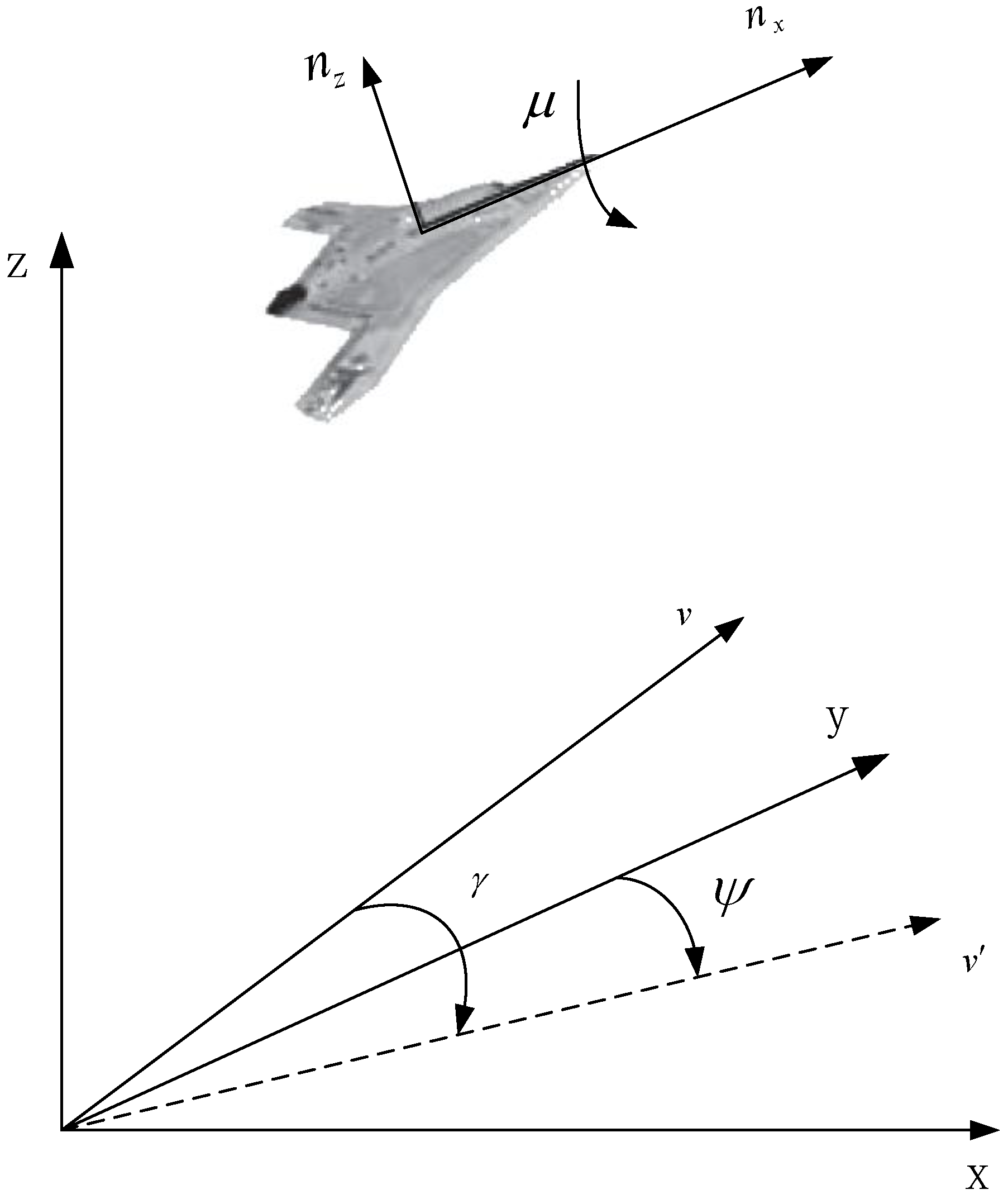
4.2. Dynamic Model for UAV

In order to control the maneuvering of the UAV, the motion model must be established. We use a three-degrees-of-freedom particle model to describe the UAV. The ground coordinate system is shown in Figure 3. The $ox$ axis points to the east, the $oy$ axis points to the north, and the $oz$ follows the right-hand rule of the coordinate axis. The motion model of the UAV in the coordinate system is shown as follows:

$$\{\begin{array}{c}\dot{x}=v\cos \gamma \sin \psi \\ \dot{y}=v\cos \gamma \cos \psi \\ \dot{z}=v\sin \gamma \end{array}$$

(2)

where x, y, and z represent the position of the UAV in the coordinate system, $v$ represents speed, and $\dot{x},\dot{y}$, and $\dot{z}$ are the component values of the speed $v$ on the three coordinate axes. The track angle $\gamma$ denotes the angle between the velocity vector and the $oxy$ plane. The projection of $v$ on the $oxy$ plane is denoted as $v^{\prime }$. The heading angle $\psi$ is the angle between the $v^{\prime }$ and $oy$ axis. In the same coordinate system, the dynamic model for the UAV can be shown as:

$$\{\begin{array}{l}\dot{v}=g(n_x-\sin \gamma )\\ \dot{\gamma }=\frac{g}{v}(n_z\cos \mu -\cos \gamma )\\ \dot{\psi }=\frac{g{n}_z\sin \mu }{v\cos \gamma }\end{array}$$

(3)

where g is the acceleration of gravity, $n_x$ is the overload in the velocity direction, $n_z$ is the overload in the pitch direction, and $\mu$ is the roll angle around the velocity $v$. $[n_x,n_z,\mu ]\in R^3$ represent the feasible basic control parameters in the UAV maneuver control model.

4.3. State Space

The state space of this scenario has two components. One component is the states of the enemy aircraft. Because we do not control the enemy aircraft, it can be seen as a mass point. The state of each enemy aircraft has six dimensions to denote its position and velocity, which are denoted as $[x,y,z,\dot{x},\dot{y},\dot{z}]$. In the experiment, the enemy aircraft fly toward the UAV with a velocity of 150 m/s. The other component of the state space is the states for the UAV. Besides the position and velocity, the states of the UAV also include the track angle $\gamma$ and heading angle $\psi$, denoted as $[x,y,z,\dot{x},\dot{y},\dot{z},\gamma ,\psi ]$. In order to facilitate the training of the neural network, each component of the states is normalized to $[0,1]$ before being fed into the input layer.

4.4. Action Space

As we have discussed above, the action space for the UAV is $[n_x,n_z,\mu ]\in R^3$. This is a continuous action space. In order to reduce the complexity of the problem, we employ the idea from [17] and discretize the UAV action space into 15 actions. To move in different directions, the UAV can take five types of actions: forward, right-turn, left-turn, upward, and downward. Additionally, it can take three velocity types of action for each direction: deceleration, maintain, and accelerate. This is shown in

Table 1. Maneuver library.

Maneuver	Control Values
	nx	nz	μ
forward maintain	0	1	0
forward accelerate	2	1	0
forward decelerate	−1	1	0
left turn maintain	0	8	−arccos(1/8)
left turn accelerate	2	8	−arccos(1/8)
left turn decelerate	−1	8	−arccos(1/8)
right turn maintain	0	8	arccos(1/8)
right turn accelerate	2	8	arccos(1/8)
right turn decelerate	−1	8	arccos(1/8)
upward maintain	0	8	0
upward accelerate	2	8	0
upward decelerate	−1	8	0
downward maintain	−1	8	$\pi$
downward accelerate	2	8	$\pi$
downward decelerate	−1	8	$\pi$

.

At each time step in the training process, the agent selects an action $a\in A$ using the $\epsilon -greedy$ method. This means that the action with the highest value function is selected with a probability of $1-\epsilon$, and the action is selected randomly with a probability of $\epsilon$ to trade-off for exploration and exploitation. During the test process, the agent selects an action with the highest value function. The agent control vector can be determined by referencing Table 1 with Equations (4) and (5) as shown below.

$$A=\left\{a_1,a_2,\cdots ,a_m\right\},m=15$$

(4)

$$a_i=[n_x,n_y,\mu ],i=1,2,\cdots ,15$$

(5)

4.5. Reward Function

Finally, if the agent can reach the target, then the reward of 1 is granted to the agent. If the agent crashes with enemy aircraft, then it gets a reward of −10. Otherwise, the agent gets 0, which can be shown as follows:

$$r_t=\{\begin{array}{l}1,if{\Vert s_t-G\Vert }_2\le 100\\ -10,if{\Vert s_t-c_t\Vert }_2\le 100\\ 0,\mathrm{otherwise}\end{array}$$

where $s_t$ denotes the position of the UAV at timestep t, which includes the seventh to the ninth dimensions of the state vector, and $c_t$ denotes the position of the enemy aircraft, which includes the first three dimensions of the state vector.

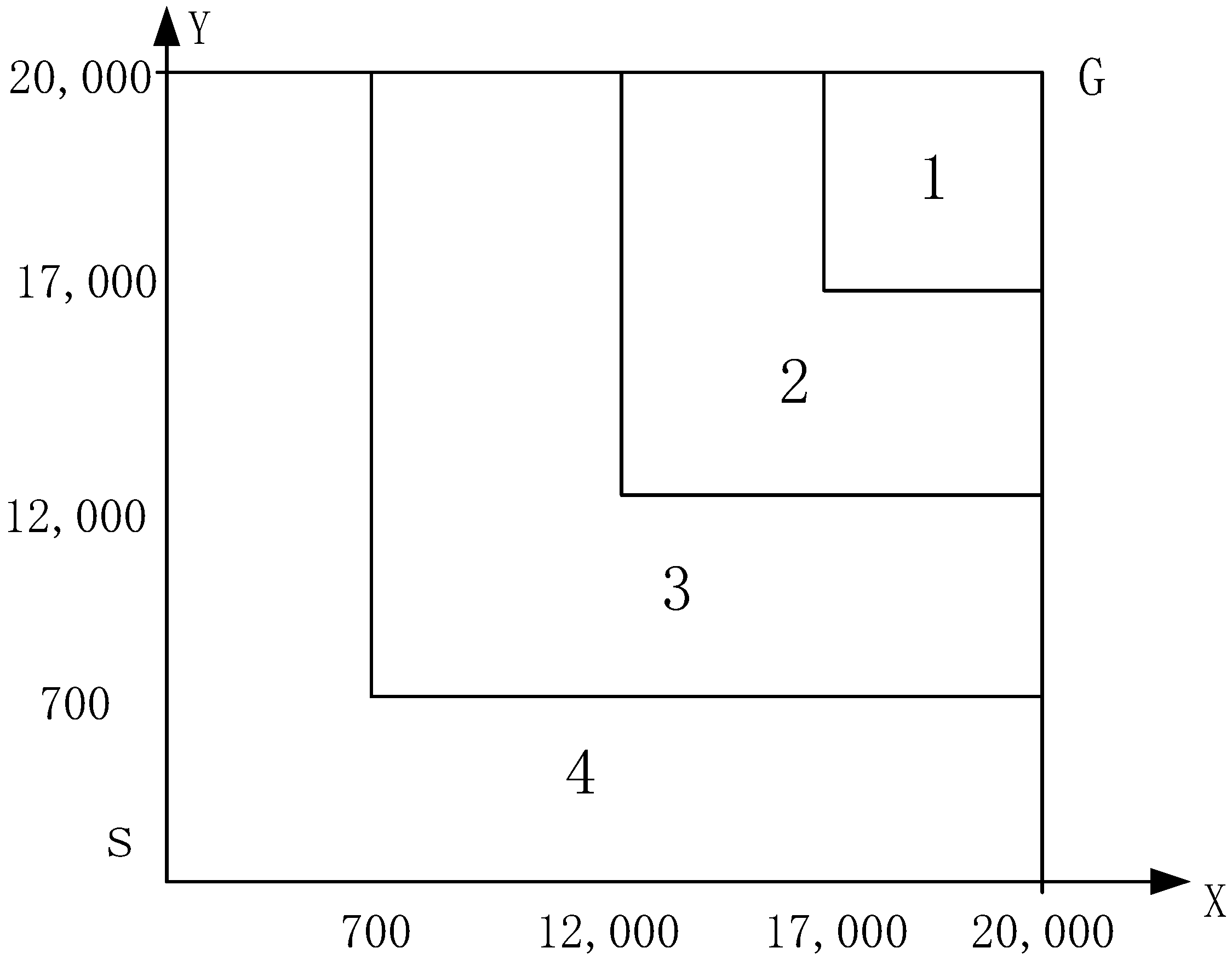
4.6. The Distributions of the Initial State

In this study, we designed the curriculum learning for the agent by setting the distribution of the initial state $s_0$ to be close to the goal in the early training stage. With this method, the agent has a greater chance of reaching the goal and receiving the informative reward. As the training process continues, the initial state is set farther away from the goal. Designing the curriculum in this way is direct and intuitive. Heuristically, we divided the $oxy$ plane of the air combat field into four parts, denoted as 1, 2, 3, and 4, respectively, as shown in Figure 4. Firstly, the initial state is set to be uniformly distributed in the No. 1 area in the combat field. Then, it is set in the No. 2 area, and so on, until it goes to the same origin as the task originally set. The threshold value $\Gamma$, which counts the successful trajectories for each area, is set as 50. This means if the agent collects 50 trajectories that fulfill the task, the initial state moves to the next area.

4.7. Network Architecture for the Value Function

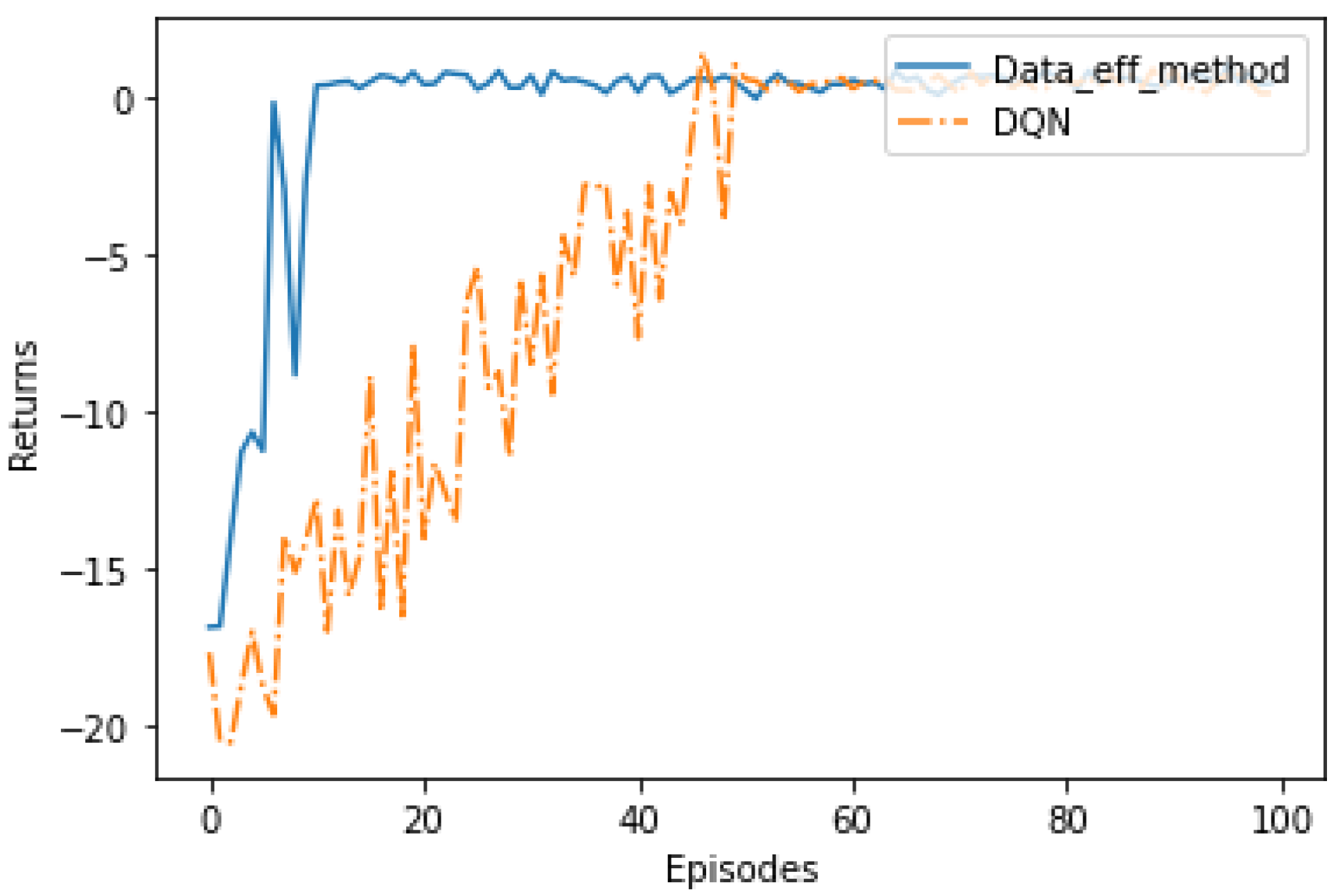
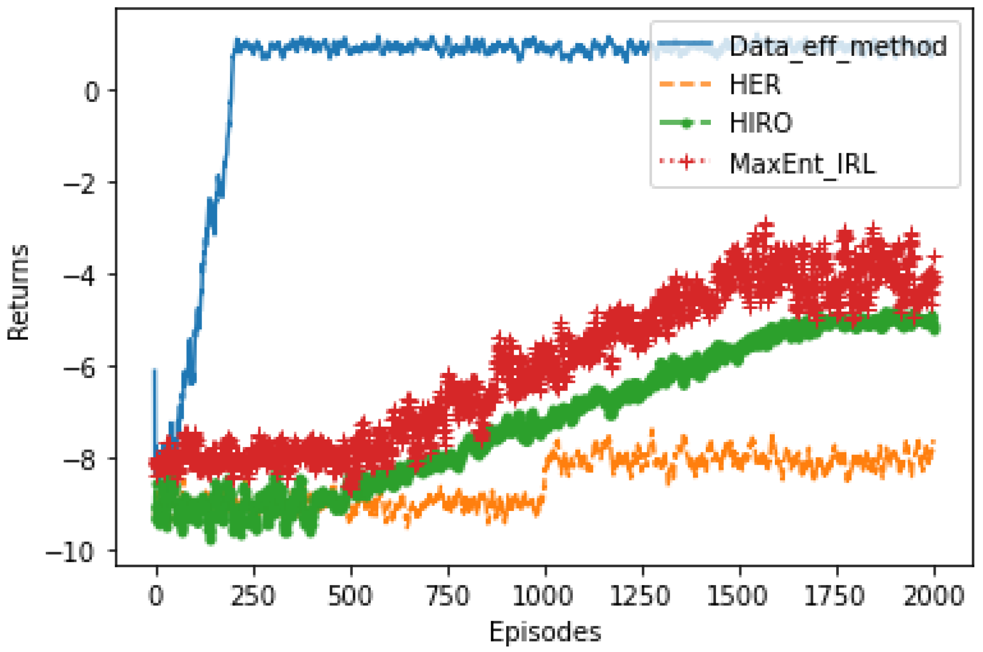
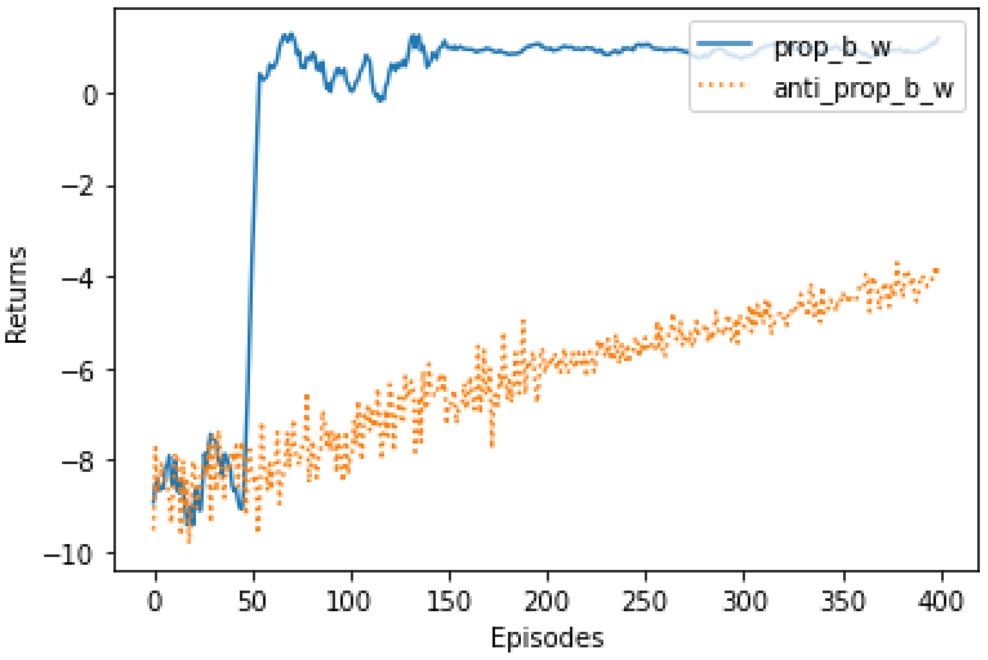
The DQN algorithm is applied to train the agent. A fully connected neural network with three hidden layers is used to present the value function. The input layer has 14 units for the dimension of the state space, and the output layer has 15 units for that of the action space. The units for the hidden layers are 128, 512, and 64. The output layer is a linear transformation, and the activation functions for the other layers are ReLU. We summarize all the hyperparameters used in the study in

Table 2. Hyperparameters of the experiment.

Hyperparameter	Value
Threshold for win trajectories $\Gamma$	50
Parameter for $\epsilon -decay$	0.005
Parameter for $p(B_w)$ decay $\tau$	0.95
Discounting rate $\gamma$	0.98
Units for the NN	(14, 128, 512, 64, 15)
Learning rate $\alpha$	0.002
Update the target net every d steps	100
Buffer size for the two experiment replays	5000
Minibatch size	64
Max velocity for the UAV	200 m/s
Min velocity for the UAV	80 m/s

.

5. Results

We compare our training framework with three state-of-the-art methods from the DRL community. They are HER [39], HIRO [38], and MaxEnt_IRL [32]. We discussed HER in Section 2. HIRO is hierarchical reinforcement learning with hindsight experiment replay, which uses a multi-layer policy to divide the task into multiple short-horizon ones. For the curriculum learning, [32] designed the curriculum without human interference. Figure 5 shows the learning curves for these four methods. The results are averaged for 30 rounds.

It can be seen from the learning curves that the proposed method in this study can obtain a good result in 196 episodes. After interacting with the environment for about 70 episodes in the first curriculum, the agent does a good job in this easy scenario. Then, when the agent interacts with a new curriculum, the learning curve shows that the performance degrades significantly. However, the agent can catch up within a few episodes. The other methods cannot converge within 2000 episodes.

As mentioned above, the efficiency of the training data is different in different training stages. In the early stage, the agent needs data from successful trajectories to know how to complete the task. Data from success trajectories are valuable in this training stage. As the training processes occur, the agent needs to know which actions are wrong for the task. Therefore, data from failure trajectories should be fed to the algorithm to encourage the agent to explore the state space widely. In contrast to the data-efficient training method discussed above, we conducted another experiment in which more failure trajectories are fed to the algorithm in the first training stage. Then, we increased the successful trajectories during the training process. The learning curve of this method and that of our proposed method can be shown in Figure 6, showing that this additional method learns more slowly than our proposed method does.

The experiment was run on a computer with an Intel^® Core™ i7-8700k CPU with 16 GB of RAM, and an NVIDIA GeForce RTX 2060 graphics card was also installed for Pytorch acceleration. We present the time cost and total return in

Table 3. Time cost and total return.

Method	Time Cost	Total Return
Proposed data-efficient framework	28 m	0.95
HER	43 m	−7.3
HIRO	47 m	−5.4
MaxEntIRL	21 m	−3.2

.

6. Conclusions and Future Work

In this paper, we proposed a data-efficient training method for DRL. We designed a curriculum for the agent in the simulation environment. Because we set the distribution of the initial state heuristically, the agent is not only more likely to receive an informative reward, but also explore state spaces it rarely explored in previous trajectories as led by the learned policy. Specifically, as the training process occurs, we set the initial state to be uniformly distributed in the designed space. The state space was not explored thoroughly by the agent when it was led by the policies trained with conventional methods. This may be another reason why the proposed method can find the proper policy quickly and precisely.

Data inefficiency is a well-known obstacle for DRL when it is applied widely in industry. We found that data efficiency is different between different training processes, even for the same data. Data from successful trajectories are more efficient in the early training stage.

Establishing a data-efficient training method has significant value for applying DRL to industrial control fields. Collecting the training data for DRL is costly and time consuming in reality. Even in simulation environments, training DRL algorithms with a conventional roadmap requires vast amounts of data. Additionally, taking weeks to train the algorithms is often prohibitive. The data-efficient learning methods presented in this study make the DRL algorithms applicable for use in complex industrial control fields.

We used DQN as the base training algorithm in our training methods. Theoretically, many other RL algorithms can be deployed in the present training framework. Designing experiments for the other RL algorithms as base training algorithms within the proposed data-efficient training methods is our first potential future research direction. The techniques used to design the curriculum for the DRL algorithm are heuristic. Although they work well in many real fields, laying the theoretical foundation for the curriculum design is our second potential research direction.

References

1. Mnih, V.; Badia, A.P. Human-level control through deep reinforcement learning. Nature 2015, 518, 529–533. [Google Scholar] [CrossRef] [PubMed]
2. Silver, D.; Schrittwieser, J.; Simonyan, K.; Antonoglou, I.; Huang, A.; Guez, A.; Hubert, T.; Baker, L.; Lai, M.; Bolton, A.; et al. Mastering the game of Go without human knowledge. Nature 2017, 550, 354–359. [Google Scholar] [CrossRef] [PubMed] [Green Version]
3. Silver, D.; Hubert, T.; Schrittwieser, J.; Antonoglou, I.; Lai, M.; Guez, A.; Lanctot, M.; Sifre, L.; Kumaran, D.; Graepel, T.; et al. A general reinforcement learning algorithm that masters chess, shogi, and go through self-play. Science 2018, 362, 1140–1144. [Google Scholar] [CrossRef] [Green Version]
4. Moravčík, M.; Schmid, M.; Burch, N.; Lisý, V.; Morrill, D.; Bard, N.; Davis, T.; Waugh, K.; Johanson, M.; Bowling, M. DeepStack: Expert-Level Artificial Intelligence in No-Limit Poker. Scence 2017, 356, 508–513. [Google Scholar] [CrossRef] [Green Version]
5. Brown, N.; Sandholm, T. Safe and nested subgame solving for imperfect-information games. arXiv 2017, arXiv:1705.02955. [Google Scholar]
6. Jaderberg, M.; Czarnecki, W.M.; Dunning, I.; Marris, L.; Lever, G.; Castañeda, A.G.; Beattie, C.; Rabinowitz, N.; Morcos, A.; Ruderman, A.; et al. Human-level performance in 3D multiplayer games with population-based reinforcement learning. Science 2019, 364, 859–865. [Google Scholar] [CrossRef] [PubMed] [Green Version]
7. Vinyals, O.; Babuschkin, I.; Czarnecki, W.M.; Mathieu, M.; Dudzik, A.; Chung, J.; Choi, D.H.; Powell, R.; Ewalds, T.; Georgiev, P.; et al. Grandmaster level in StarCraft II using multi-agent reinforcement learning. Nature 2019, 575, 350–354. [Google Scholar] [CrossRef]
8. Kober, J.; Bagnell, J.A.; Peters, J. Reinforcement learning in robotics: A survey. Int. J. Robot. Res. 2013, 32, 1238–1274. [Google Scholar] [CrossRef] [Green Version]
9. Levine, S.; Finn, C.; Darrell, T.; Abbeel, P. End-to-End Training of Deep Visuomotor Policies. J. Mach. Lean. Res. 2016, 17, 1334–1373. [Google Scholar]
10. Kalashnikov, D.; Irpan, A.; Pastor, P.; Ibarz, J.; Herzog, A.; Jang, E.; Quillen, D.; Holly, E.; Kalakrishnan, M.; Vanhoucke, V.; et al. QT-Opt: Scalable Deep Reinforcement Learning for Vision-Based Robotic Manipulation. arXiv 2018, arXiv:1806.10293. [Google Scholar]
11. Pinto, L.; Gupta, A. Supersizing self-supervision: Learning to grasp from 50K tries and 700 robot hours. In Proceedings of the 2016 IEEE International Conference on Robotics and Automation (ICRA), Stockholm, Sweden, 16–21 May 2016; pp. 3406–3413. [Google Scholar]
12. Nagabandi, A.; Konoglie, K.; Levine, S.; Kumar, V. Deep Dynamics Models for Learning Dexterous Manipulation. In Proceedings of the 2020 Conference on Robot Learning, Virtual, 16–18 November 2020; pp. 1101–1112. [Google Scholar]
13. Kalashnikov, D.; Varley, J.; Chebotar, Y.; Swanson, B.; Jonschkowski, R.; Finn, C.; Levine, S.; Hausman, K. MT-Opt: Continuous Multi-Task Robotic Reinforcement Learning at Scale. arXiv 2021, arXiv:2104.08212. [Google Scholar]
14. Gupta, A.; Yu, J.; Zhao, T.Z.; Kumar, V.; Rovinsky, A.; Xu, K.; Devlin, T.; Levine, S. Reset-Free Reinforcement Learning via Multi-Task Learning: Learning Dexterous Manipulation Behaviors without Human Intervention. arXiv 2021, arXiv:2104.11203. [Google Scholar]
15. Degrave, J.; Felici, F.; Buchli, J.; Neunert, M.; Tracey, B.; Carpanese, F.; Ewalds, T.; Hafner, R.; Abdolmaleki, A.; de las Casas, D.; et al. Magnetic control of tokamak plasmas through deep reinforcement learning. Nature 2022, 602, 414–419. [Google Scholar] [CrossRef] [PubMed]
16. Mirhoseini, A.; Goldie, A.; Yazgan, M.; Jiang, J.W.; Songhori, E.; Wang, S.; Lee, Y.; Johnson, E.; Pathak, O.; Nazi, A.; et al. A graph placement methodology for fast chip design. Nat. Int. Wkly. J. Sci. 2021, 594, 207–212. [Google Scholar] [CrossRef]
17. Hu, J.; Wang, L.; Hu, T.; Guo, C.; Wang, Y. Autonomous Maneuver Decision Making of Dual-UAV Cooperative Air Combat Based on Deep Reinforcement Learning. Electronics 2022, 11, 467. [Google Scholar] [CrossRef]
18. Rusu, A.A.; Vecerik, M.; Rothörl, T.; Heess, N.; Pascanu, R.; Hadsell, R. Sim-to-Real Robot Learning from Pixels with Progressive Nets. arXiv 2016, arXiv:1610.042868. [Google Scholar]
19. Zhao, W.; Queralta, J.P.; Westerlund, T. Sim-to-Real Transfer in Deep Reinforcement Learning for Robotics: A Survey. In Proceedings of the 2020 IEEE Symposium Series on Computational Intelligence (SSCI), Canberra, Australia, 1–4 December 2020; pp. 737–744. [Google Scholar]
20. Bellemare, M.G.; Naddaf, Y.; Veness, J.; Bowling, M. The Arcade Learning Environment: An Evaluation Platform for General Agents. J. Artif. Intell. Res. 2012, 47, 253–279. [Google Scholar] [CrossRef]
21. Machado, M.C.; Bellemare, M.G.; Talvitie, E.; Veness, J.; Hausknecht, M.; Bowling, M. Revisiting the Arcade Learning Environment: Evaluation Protocols and Open Problems for General Agents. J. Artif. Intell. Res. 2018, 61, 523–562. [Google Scholar] [CrossRef]
22. Schulman, J.; Wolski, F.; Dhariwal, P.; Radford, A.; Klimov, O. Proximal Policy Optimization Algorithms. arXiv 2017, arXiv:1707.06347. [Google Scholar]
23. Hessel, M.; Modayil, J.; van Hasselt, H.; Schaul, T.; Ostrovski, G.; Dabney, W.; Horgan, D.; Piot, B.; Azar, M.; Silver, D. Rainbow: Combining Improvements in Deep Reinforcement Learning. In Proceedings of the Thirty-Second AAAI Conference on Artificial Intelligence, New Orleans, LA, USA, 2–7 February 2018. [Google Scholar]
24. Tsividis, P.A.; Tenenbaum, J.B.; Pouncy, T.; Xu, J.; Gershman, S. Human learning in atari. In Proceedings of the AAAI Spring Symposium—Technical Report, Standford, CA, USA, 27–29 March 2017. [Google Scholar]
25. Fedus, W.; Ramachandran, P.; Agarwal, R.; Bengio, Y.; Larochelle, H.; Rowland, M.; Dabney, W. Revisiting Fundamentals of Experience Replay. In Proceedings of the International Conference on Machine Learning, Virtual, 12–18 July 2020; pp. 3061–3071. [Google Scholar]
26. Zhang, S.; Sutton, R.S. A Deeper Look at Experience Replay. arXiv 2017, arXiv:1712.01275. [Google Scholar]
27. Silver, D.; Singh, S.; Precup, D.; Sutton, R.S. Reward is enough. Artif. Intell. 2021, 299, 103535. [Google Scholar] [CrossRef]
28. Sutton, R.; Barto, A. Reinforcement Learning: An Introduction; MIT Press: Cambridge, MA, USA, 2018. [Google Scholar]
29. Ng, A.Y.; Harada, D.; Russell, S. Policy Invariance under Reward Transformations: Theory and Application to Reward Shaping; Morgan Kaufmann Publishers Inc.: Burlington, MA, USA, 1999. [Google Scholar]
30. Burda, Y.; Edwards, H.; Storkey, A.; Klimov, O. Exploration by Random Network Distillation. arXiv 2018, arXiv:1810.128948. [Google Scholar]
31. Badia, A.P.; Sprechmann, P.; Vitvitskyi, A.; Guo, D.; Piot, B.; Kapturowski, S.; Tieleman, O.; Arjovsky, M.; Pritzel, A.; Bolt, A.; et al. Never Give Up: Learning Directed Exploration Strategies. arXiv 2022, arXiv:2002.060388. [Google Scholar]
32. Yengera, G.; Devidze, R.; Kamalaruban, P.; Singla, A. Curriculum Design for Teaching via Demonstrations: Theory and Applications. In Proceedings of the 35th Conference in Neural Information Processing Systems, Virtual, 6–14 December 2021. [Google Scholar]
33. Wang, X.; Chen, Y.; Zhu, W. A Survey on Curriculum Learning. IEEE Trans. Pattern Anal. Mach. Intell. 2022, 49, 4555–4576. [Google Scholar] [CrossRef] [PubMed]
34. Lin, Z.; Lai, J.; Chen, X.; Cao, L.; Wang, J. Learning to Utilize Curiosity: A New Approach of Automatic Curriculum Learning for Deep RL. Mathematics 2022, 10, 2523. [Google Scholar] [CrossRef]
35. Zhipeng, R.; Daoyi, D.; Huaxiong, L.; Chunlin, C. Self-paced prioritized curriculum learning with coverage penalty in deep reinforcement learning. IEEE Trans. Neural Netw. Learn. Syst. 2018, 29, 2216–2226. [Google Scholar]
36. Gehring, J.; Synnaeve, G.; Krause, A.; Usunier, N. Hierarchical Skills for Efficient Exploration. In Proceedings of the 35th Conference in Neural Information Processing Systems, Virtual, 6–14 December 2021. [Google Scholar]
37. Vezhnevets, A.S.; Osindero, S.; Schaul, T.; Heess, N.; Jaderberg, M.; Silver, D.; Kavukcuoglu, K. FeUdal networks for hierarchical reinforcement learning. In Proceedings of the 34th International Conference on Machine Learning, Sydney, Australia, 6–11 August 2017; pp. 3540–3549. [Google Scholar]
38. Nachum, O.; Gu, S.; Lee, H.; Levine, S. Data-Efficient Hierarchical Reinforcement Learning. arXiv 2018, arXiv:1805.08296. [Google Scholar]
39. Andrychowicz, M.; Wolski, F.; Ray, A.; Schneider, J.; Fong, R.; Welinder, P.; McGrew, B.; Tobin, J.; Abbeel, P.; Zaremba, W. Hindsight Experience Replay. arXiv 2017, arXiv:1707.01495. [Google Scholar]
40. Vecchietti, L.F.; Seo, M.; Har, D. Sampling Rate Decay in Hindsight Experience Replay for Robot Control. IEEE Trans. Cybern. 2022, 52, 1515–1526. [Google Scholar] [CrossRef]
41. Schaul, T.; Horgan, D.; Gregor, K.; Silver, D. Universal value function approximators. In Proceedings of the 32nd International Conference on Machine Learning, Lille, France, 6–11 July 2015; pp. 1312–1320. [Google Scholar]
42. Levy, A.; Konidaris, G.; Platt, R.; Saenko, K. Learning multi-level hierarchies with hindsight. In Proceedings of the International Conference on Learning Representations, New Orleans, LA, USA, 6–9 May 2019. [Google Scholar]
43. Wang, J.X.; Kurth-Nelson, Z.; Tirumala, D.; Soyer, H.; Leibo, J.Z.; Munos, R.; Blundell, C.; Kumaran, D.; Botvinick, M. Learning to reinforcement learn. arXiv 2016, arXiv:1611.05763. [Google Scholar]
Figure 1. Learning curve of the toy experiment.
Electronics 11 04205 g001
Figure 2. Air combat field.
Electronics 11 04205 g002
Figure 3. Ground coordinate system for UAV.
Electronics 11 04205 g003
Figure 4. Distribution of the initial state setting in curriculum learning.
Electronics 11 04205 g004
Figure 5. Training curves of the four methods.
Electronics 11 04205 g005
Figure 6. Data efficiency in different training stages.
Electronics 11 04205 g006