Forecasting of Wind Speed and Power through FFNN and CFNN Using HPSOBA and MHPSO-BAACs Techniques

Abstract

Renewable Energy Sources are an effective alternative to the atmosphere-contaminating, rapidly exhausting, and overpriced traditional fuels. However, RESs have many limitations like their intermittent nature and availability at far-off sites from the major load centers. This paper presents the forecasting of wind speed and power using the implementation of the Feedforward and cascaded forward neural networks (FFNNs and CFNNs, respectively). The one and half year’s dataset for Jhimpir, Pakistan, is used to train FFNNs and CFNNs with recently developed novel metaheuristic optimization algorithms, i.e., hybrid particle swarm optimization (PSO) and a Bat algorithm (BA) named HPSOBA, along with a modified hybrid PSO and BA with parameter-inspired acceleration coefficients (MHPSO-BAAC), without and with the constriction factor (MHPSO-BAAC-χ). The forecasting results are made for June–October 2019. The accuracy of the forecasted values is tested through the mean absolute error (MAE), mean absolute percentage error (MAPE), and root mean square error (RMSE). The graphical and numerical comparative analysis was performed for both feedforward and cascaded forward neural networks that are tuned using the mentioned optimization techniques. The feedforward neural network was achieved through the implementation of HPSOBA with a mean absolute error, mean absolute percentage error, and root mean square error of 0.0673, 6.73%, and 0.0378, respectively. Whereas for the case of forecasting through a cascaded forward neural network, the best performance was attained by the implementation of MHPSO-BAAC with a MAE, MAPE and RMSE of 0.0112, 1.12%, and 0.0577, respectively. Thus, the mentioned neural networks provide a more accurate prediction when trained and tuned through the given optimization algorithms, which is evident from the presented results.

1. Introduction

Environmental degradation, continuously increasing atmospheric pollution, the variable prices of conventional fuels, and their rapid depletion has forced electric power producers and distributors to integrate RESs more sturdily into the existing power network [1]. RESs such as wind, with all their advantages, have the problem of being highly variable as climatic conditions keep changing. Wind power generation continues to vary, in contrast to traditional thermal power plants (TPPs), which can provide a constant power supply for longer periods [2,3]. Thus, the power extracted from wind resources has more variability as well as probability. The recurrent behavior of wind power is a substantial issue in their commissioning as a sustainable solution for the production of clean electricity. The practical answer to this problem is precise prediction of the resources for the intended regions.

Forecasting is a method that takes previous results as input to make conversant approximations that are prognostic in finding the course of upcoming tendencies [4]. Wind speed forecasting requires previous data of wind speed for the considered region along with some other environmental parameters such as temperature, relative humidity, and wind direction [5]. Generally, the estimation of wind speed is segregated into three classes: long-, medium-, and short-term estimates. The short-term forecast deals with the prediction of wind speed for a few hours, the medium-term forecast covers the forecast in the range of a few hours to some days, and the long-term forecast covers the prediction of more than three days, without any eventual limit [6]. Existing works have attempted to perform resource forecasting through many mechanisms: the application of stochastic techniques such as Rayleigh distribution (RD), Normal distribution (ND), Weibull distribution (WD), etc., and by the development of suitable neural networks (NNs).

The wind speed forecasting and power mechanism presented in this paper can be implemented to identify and calculate the design parameters of the wind turbine for a suitable region. Moreover, it can be used at the operational stage for a wind turbine as it can estimate the amount of electric power that can be collected from a wind-based system during a particular period. Hence, it optimizes the scheduling of the grid and reduces the operational costs of power plants by lowering the reserve capacity demand.

2. Literature Review

To date, various NNs have been presented for the application to different fields for the purpose of developing intelligent systems. Artificial neural networks (ANNs) are connectionist systems in which parallel operations are performed for intelligent decision making by mimicking the behavior of the human brain’s neural systems [7]. The efficiency of these NN-based schemes is due to their ability to learn and make progress in data processing, being open-minded, and being intelligent to handle nonlinear data values [8,9]. The integration of these NNs or their alternatives into the prediction system supports the sinking of the error, which guarantees that the forecast value falls in a range that maintains equilibrium in the demand and supply of real-time electricity [10]. Recent developments have employed NN-based systems in a variety of ways to perform wind forecasting for various regions around the world.

The authors of [11] offered a model which used ANNs to predict wind speeds that had seasonal and sequential topographies similar to the recorded wind data. The authors tested the model for wind speeds of Kuala Terengganu, Mersing, and Kudat in Malaysia for its verification. The results showed that the proposed system of hybrid artificial neural networks (HANNs) could demonstrate variations in wind speed for all seasons throughout the year. However, the authors did not present a detailed elaboration of the mechanism adopted for the training of the presented HANN model. The authors in [12] explored two methods for the estimation of wind power, and a detailed assessment was executed using ANNs. The authors used a hybrid forecasting method for estimating the power from wind and an extensive evaluation of the technique was conducted. The authors achieved a short-range wind power forecast for a farm of 40 wind turbine generators. The authors concluded that the ANN-based estimation method produced the projected results very quickly, but the precision and accuracy level were low. In addition, they only focused on the RMSE-based computations to check the accuracy of the considered models.

The authors of [13] presented a deep-learning-based approach for forecasting wind speed. The presented mechanism was based on multiobjective parameter optimization and hybrid time series decomposition. The results were tested through four datasets for the testing of the accuracy of the predicted values. The authors also used the Kruskal–Wallis test for checking the effectiveness of the proposed schemes, and they concluded that the performance of the given mechanisms was better than the traditional complex approaches available in the literature. In [14], a post-processing method based on time variation to perform long-term forecasting of wind speed was presented. The proposed method was based on a multiregional recurrent graph for multiregional wind speed forecasting. The results for wind speed forecasting for twenty-five real meteorological monitoring points showed that the proposed model gave a better performance in various comparative parameters.

The authors in [15] discussed turbulent wakes while trailing utility-scale wind turbines that reduce the power production and efficiency of downstream turbines. The models presented were trained through historical data of the last five years, and the values were averaged over one minute. Data were taken from the summer view wind farm in Alberta, Canada. The authors concluded that the trained models calculated a lesser error in the forecasted values in comparison to the standard two-layer neural network and physics-based wake model. In [16], a variational mode decomposition, implemented to divide the raw wind speed data into a set of intrinsic mode functions, was presented. The authors used adaptive differential evolution to optimize several important parameters for temporal fusion transformers (TFT) for prediction purposes. For the input data set, the authors used 1-hour wind speed values with eight real-world data sets in Albert, Canada. The authors concluded that the presented results indicated considerable advancement for wind speed estimation and in assisting policymakers.

The authors in [17] also developed a wind speed prediction approach, namely WindNet, founded using convolutional neural networks (CNN) for the site in Taiwan. The estimating system was developed to deliver the forecasted data for the following three days. The hourly data of the wind speed were collected for the previous week, and the dataset was established with a total of 24 × 7 = 168 sets. The designed WindNet mechanism executed 1D convolution on the accumulated data and the authors used sixteen filters that accumulated a total of 16 × 168 1D convoluted map shapes. The results were compared with the following four techniques: multilayer perception (MLP), support vector machine (SVM), decision tree (DT), and random forest (RF). RMSE and MAE were used as pointers to assess the performance of the presented architecture. However, the authors did not consider the metaheuristic techniques training mechanism of the NN. In [18], the prediction of wind through NN training using optimization techniques was presented. PSO and Levenberg–Marquardt (LM) algorithms were employed for the training of ANNs to achieve wind speed and power estimation for the short term. The performance analysis of the considered techniques was conducted only through the computation of the MAPE. The authors in [19] performed a detailed study of wind resource forecasting through the Weibull distribution (WD) directly or through integration with other mechanisms, as presented in the recent literature. In [20,21], the RNN-LSTM algorithm was proposed for day-ahead wind energy generation.

HPSOBAs and MHPSO-BAACs are recently developed metaheuristic optimization algorithms that have successfully solved the EDPs for various cases of constrained and non-constrained TPPs, HPSs, and RESs presented in [22,23]. The results presented lower dispatch cost values, better convergence, and lesser computational times. However, to make RES-based power systems sustainable and carry the major load, the forecasting of RESs is essential.

Research Contribution

The work in this paper presents the following contributions to the literature:

• A wind speed and its respective power estimation model were designed using FFNN and CFNN trained through the recently developed metaheuristic optimization algorithms HPSOBAs, MHPSO-BAACs, and the standard PSO.
• The forecasting is performed for the five months (June to October 2019) using the historical data from January 2018 to May 2019.
• The accuracy of the forecasted values is tested through an error-testing formulation based on the MAE, MAPE, and RMSE.
• To have a fair comparison of the considered NNs for the wind speed and its respective power prediction in the Jhimpir region, training techniques, parameters, the number of layers, and input values are considered the same.
• The presented comparison of the results authenticates the better and more accurate performance of the FFNN and CFNN when trained through MHPSO-BAACs, HPSOBAs, and PSOs.
• The presented work, if implemented, can help in enhancing the contribution of wind-turbine-based power generation systems.

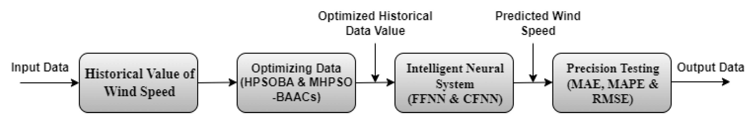
The structural block diagram of the wind speed forecasting model presented in this paper is given in Figure 1.

The organization of the paper is as follows: Section 3 presents the system model and mathematical formulations, followed by the review of the NN and optimization techniques considered in Section 4; Section 5 discusses the proposed research methodology; the results and discussion is given in Section 6; Section 7 concludes the article, followed by the cited references.

3. Mathematical Formulations

This section provides an overview of the mathematical formulations employed, the considered NNs, and the optimization techniques employed to train the FFNN. The subsections also provide an overview of the standard PSO algorithm, as it is also used to train the NNs for the comparison of the results. At the end of this section, a detailed explanation of the design application of the system model is provided. The objective function employed for the wind speed and its respective power estimation is given by

$$Objective Function = \frac{1}{N}{\displaystyle \sum _{i=1}^N{\left(\left(v_{i,o}\right)-\left(v_{i,t}\right)\right)}^2},$$

(1)

where v_i,o and v_i,t designate the observed or measured velocity as the input and target for the neural networks (NNs), respectively. The mathematical representation of the FFNN and CFNN is given by [24,25]

$$v_k={\displaystyle \sum _{i=1}^N{W}_{ki}{X}_i}$$

(2)

and

$$y = {\displaystyle \sum _{i=1}^N{f}^i{\omega }_i^i{x}_i+f^o\left({\displaystyle \sum _{j=1}^k{\omega }_j^o{f}_j^h}\left({\displaystyle \sum _{i=1}^N{\omega }_{ji}^h}{x}_i\right)\right)}.$$

(3)

The mathematical formula for the calculation of the predicted wind power by using the forecast wind speed is given as

$$P=\left(\frac{1}{2}\right)\rho A{C}_p{v}^3,$$

(4)

where A gives the swept area of the wind turbines, Cp gives the performance coefficient, $\rho$ gives the air density (kg/m³), and v designates the wind speed [26,27].

The mean absolute error (MAE), mean absolute percentage error (MAPE), and root mean square error (RMSE) are used to authenticate the accuracy of the forecasted values. Mathematically, the MAE, MAPE, and RMSE are given by [28]:

$$MAE=\left(\frac{1}{n}\right){\displaystyle \sum _{i=1}^N\left|A{v}_i-E{v}_i\right|},$$

(5)

$$MAPE=\left(\frac{1}{n}\right){\displaystyle \sum _{i=1}^N\left|\frac{A{v}_i-E{v}_i}{A{v}_i}\right|}\times 100,$$

(6)

and

$$RMSE={\left[\left(\frac{1}{n}\right){\displaystyle \sum _{i=1}^N{\left(A{v}_i-E{v}_i\right)}^2}\right]}^{\frac{1}{2}},$$

(7)

where E_vi and A_vi are the estimated and real values for ith data, respectively, and the total number of samples is represented by N [29,30,31]. The proceeding subsection reviews the FFNN considered for the estimate of the wind speed and the optimization techniques used to train them [32].

4. Neural Network and Optimization Techniques

This section provides an overview of the considered artificial neural network (ANN), along with the HPSOBA and MHPSO-BAACs optimization techniques used to train the FFNN. The subsections also provide an overview of the standard PSO algorithm as it is also used to train the NNs for the aim of comparison. At the end of this section, a detailed explanation of the design application of the system model is provided.

4.1. Feedforward Neural Network (FFNN)

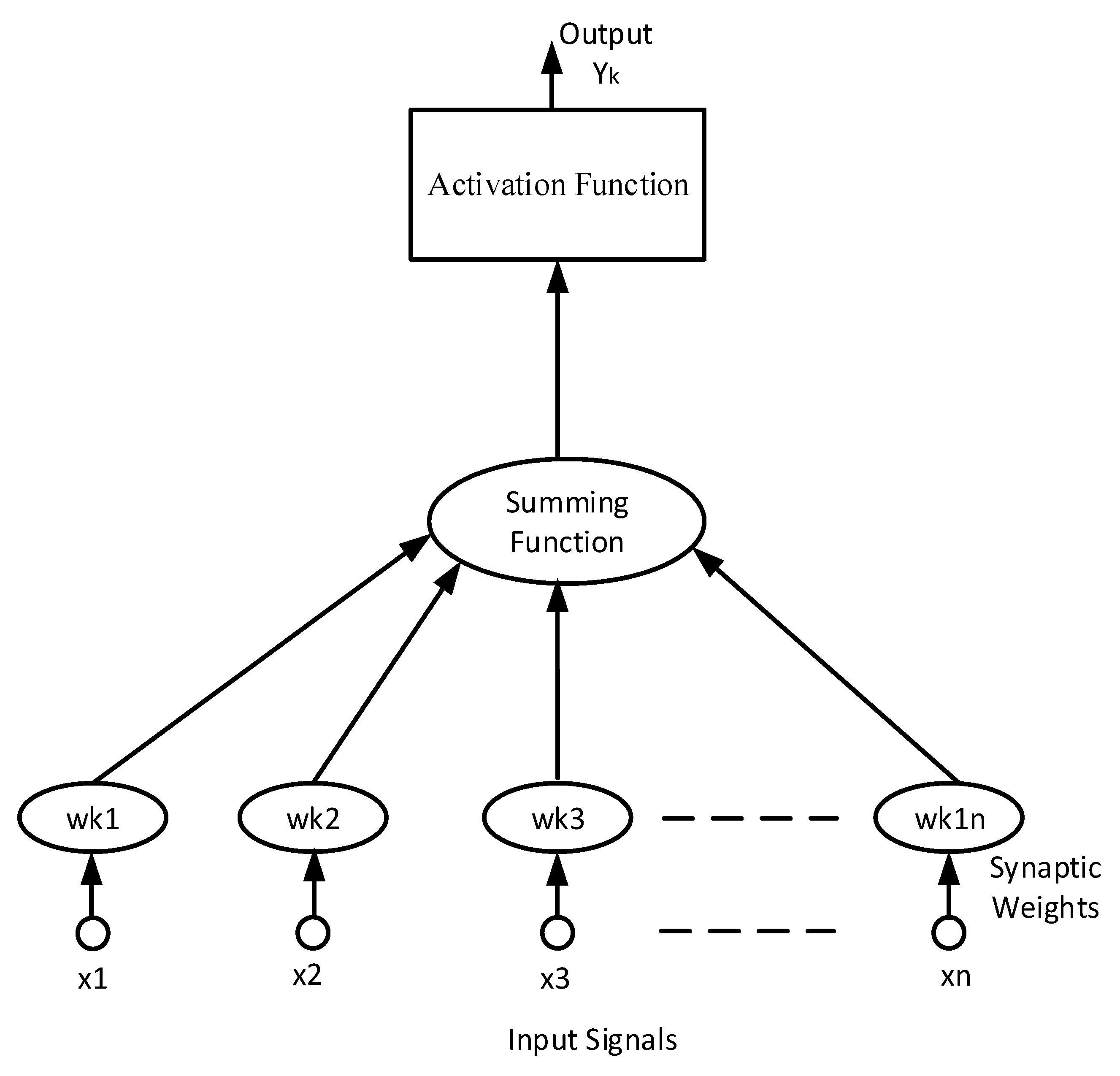
The FFNN is a biologically stimulated classification algorithm. It consists of neurons that act as the processing units and are structured in layers, and every neuron in the layer is linked to all the units of the preceding layers. Data enters the input and moves forward in the network through the layers until it arrives at the output layer. In the standard process of FFNN, it works as a classifier and has no feedback between layers, giving them the name of a feedforward neural network [33,34]. The nodal operation of the FFNN is explained in Figure 2.

4.2. Cascaded Forward Neural Network (CFNN)

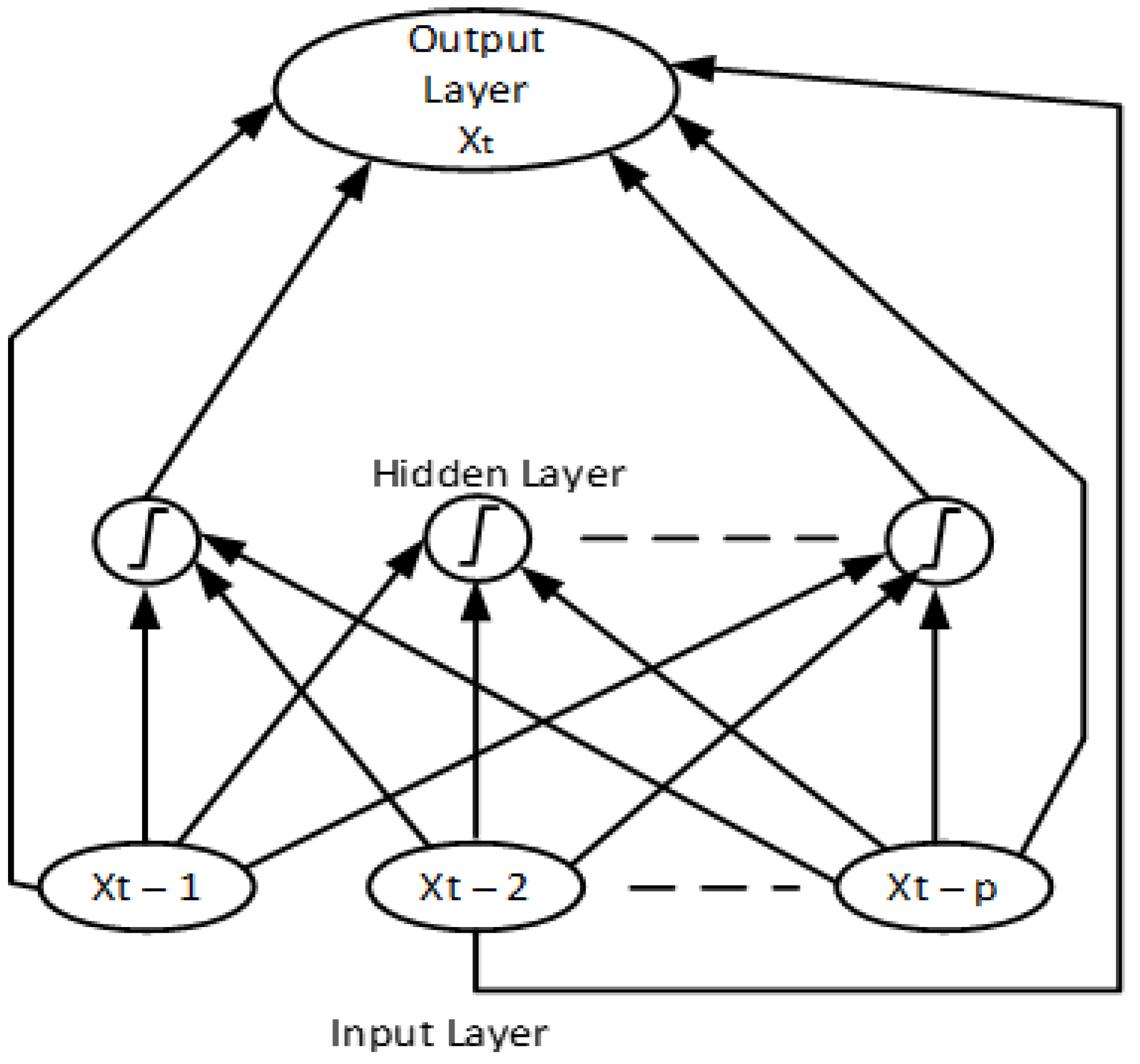
When the connection from the perspicacity and multilayer network is integrated, the system has direct linking where the input and output layers are shaped. Such a designed system is called the CFNN [35]. The perceptron and link that is shaped between the input and output layers of CFNN is a method of direct relation. On the other hand, for FFNN, the linkage established among the input and output layers is due to an indirect connection. The architecture of the CFNN is given in Figure 3.

4.3. Particle Swarm Optimization (PSO)

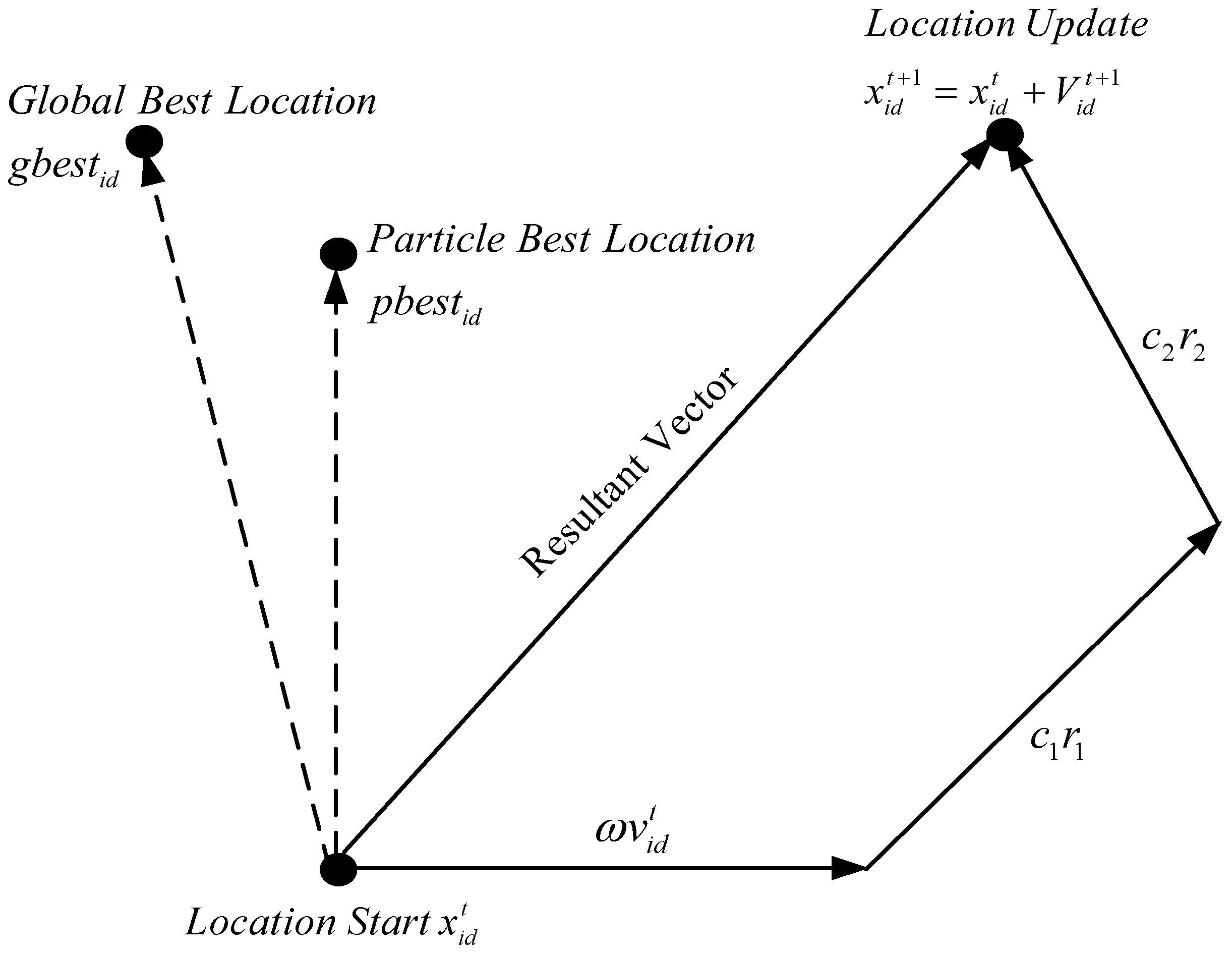
PSO is a metaheuristic optimization process that is applied to achieve the appropriate result for optimization glitches, and was suggested by Kennedy in 1995. PSO is founded on the imitation of the swarm of birds flying in multidimensional space to hunt a suitable place, regulating their explorations in the designated space for an improved search. To solve optimization problems, it is the most effective method but has a feebleness such that it may stick in the local minima. Modern research have strived to enhance the operational capability of PSO by relocating or integrating new variables into the original formulation. The presented research tried improving the performance through the refinement of the loading of the group of particles, and some integrated different factors such as the constriction factor and inertial weight, etc. In addition, the best global and local particles were also used for the mutation operation [36]. Pictorially, PSO is given in Figure 4.

Figure 2 shows the intellectualized vector diagram that relates the particle movement with the PSO equations. Equations (8) and (9) provide the mathematical representation of the position and velocity parameters of standard PSO,

$$v_{id}^{t+1}=\stackrel{Inertial Component}{\overbrace{\omega v_{id}^t}}+ \stackrel{Cognitive Component}{\overbrace{c_1{r}_1(pbes{t}_{id}-x_{id}^t)}} + \stackrel{Social Component}{\overbrace{c_2{r}_2(gbes{t}_{gd}-x_{id}^t)}},$$

(8)

and

$$x_{id}^t=x_{id}^t+v_{id}^{t+1}, \mathrm{with} i=1,2,\dots ,n; \mathrm{while} d=1,2,\dots ,m,$$

(9)

where i is the index term of the particle, t is the index term of the discrete time, n and m give the number and dimensions of the particles in a group, respectively, d gives the considered dimension, ω represents the inertia weight factor, r₁ and r₂ are the randomization parameters, and c₁ and c₂ are the coefficients of cognitive and social acceleration, respectively [34,35,36,37].

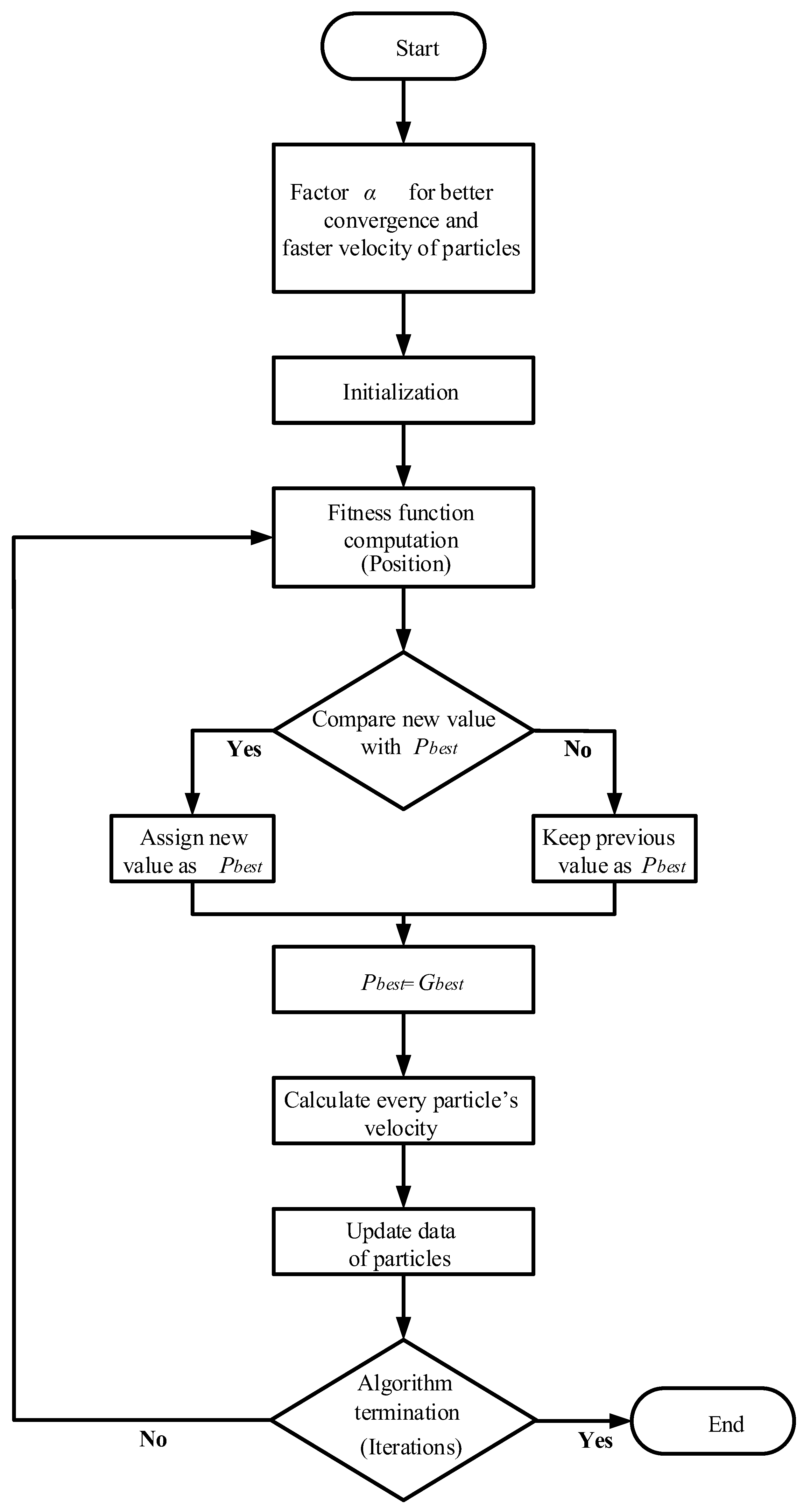
4.4. Hybrid PSO and BA (HPSOBA)

The HPSOBA is a flexible and unique algorithm that combines the important features of the classical BA and PSO algorithms. The developed procedure presented the best solutions for EDP for different groups of RESs and TPPs [37]. The mathematical formulation for the velocity and position parameters of the HPSOBA is presented in (10) and (11), respectively:

$$v_{id}^{t+1}=\alpha \times \left(\omega v_{id}^t+c_1{r}_1(pbes{t}_{id}-x_{id}^t)+ c_2{r}_2(gbes{t}_{gd}-x_{id}^t)\right);$$

(10)

$$x_i^{t+1}=\left(1-r\right)x_i^t+r{p}_{best}{}_{{}_i}+v_i^{t+1}.$$

(11)

The process is designed by integrating two parameters in the velocity equation of the standard PSO: a novel and distinctive variable α given in Equation (12),

$$\alpha =\left(\raisebox{1ex}{$c$}\!\left/ \!\raisebox{-1ex}{$r$}\right.\right)f.$$

(12)

The new parameter α is computed using the cognitive social component c and the random pdf r of the standard PSO. Meanwhile, f is the frequency of BA while the ranges remain the same as in the standard form. Commonly, c₁ and c₂ are considered of the same value, and thus c has the same value for calculation in (12). The inertial weight parameter ω is computed using Equation (13) [38]:

$$\omega ={\omega }_{\min }+\left[{\omega }_{\max }-\left(\frac{{\omega }_{\max }-{\omega }_{\min }}{ite{r}_{\max }}\right)iter\right]r.$$

(13)

The considered value of the random pdf r is the same for both the variables α and ω. The pseudocode and the flowchart of the HPSOBA are presented in Figure 5 and Algorithm 1 [19].

Algorithm 1. Hybrid PSO and BA (HPSOBA).

1: Initiate factors: population, frequency, iterations, and inertia weight

2: Initialization of position and velocity

3: for i = 1:npop

4:       Set position

5:       set velocity

6:             apprise Pbest for position, velocity and yield

7:           apprise Gbest

8:                 if finest result of velocity > finest velocity

9:                  Velocity = finest result;

10:               end if

11:                end for

12: HPSOBA main loop:

13: for iteration = 1:maxit

14:       for i = 1:npop

15:                 Compute ω and alpha

16:                            $\omega ={\omega }_{\min }+\left[{\omega }_{max}-\left(\frac{{\omega }_{max}-{\omega }_{\min }}{ite{r}_{max}}\right)iter\right]r$

17:                          $\alpha \leftarrow (c/r)f$

18:                     Update velocity:

19:                            $v_{id}^{t+1}=\alpha \left(\omega v_{id}^t+ c_1{r}_1·(pbes{t}_{id}-x_{id}^t)+c_2{r}_2·(gbes{t}_{id}-x_{id}^t)\right)$

20:                         Update position:

21:                                    $x_i^{t+1}=\left(1-r\right)x_i^t+r{P}_{best,i}+v_i^{t+1}$

22:                         Apprise Pbest:

23:                                                          if velocity < finest velocity

24:                                                                  position = finest position;

25:                                                                  velocity = finest velocity;

26:                                                                  output = finest output;

27:                         Apprise Gbest

28:                                                          if finest result of velocity > finest velocity

29:                                                                   finest velocity = finest result

30:                                                          end if

31:                                                       end if

32:                             end for

33: Optimal Cost (iteration) = Optimal Result;

34: Display (iteration, Optimal Solution);

35: end for

36: Plot results

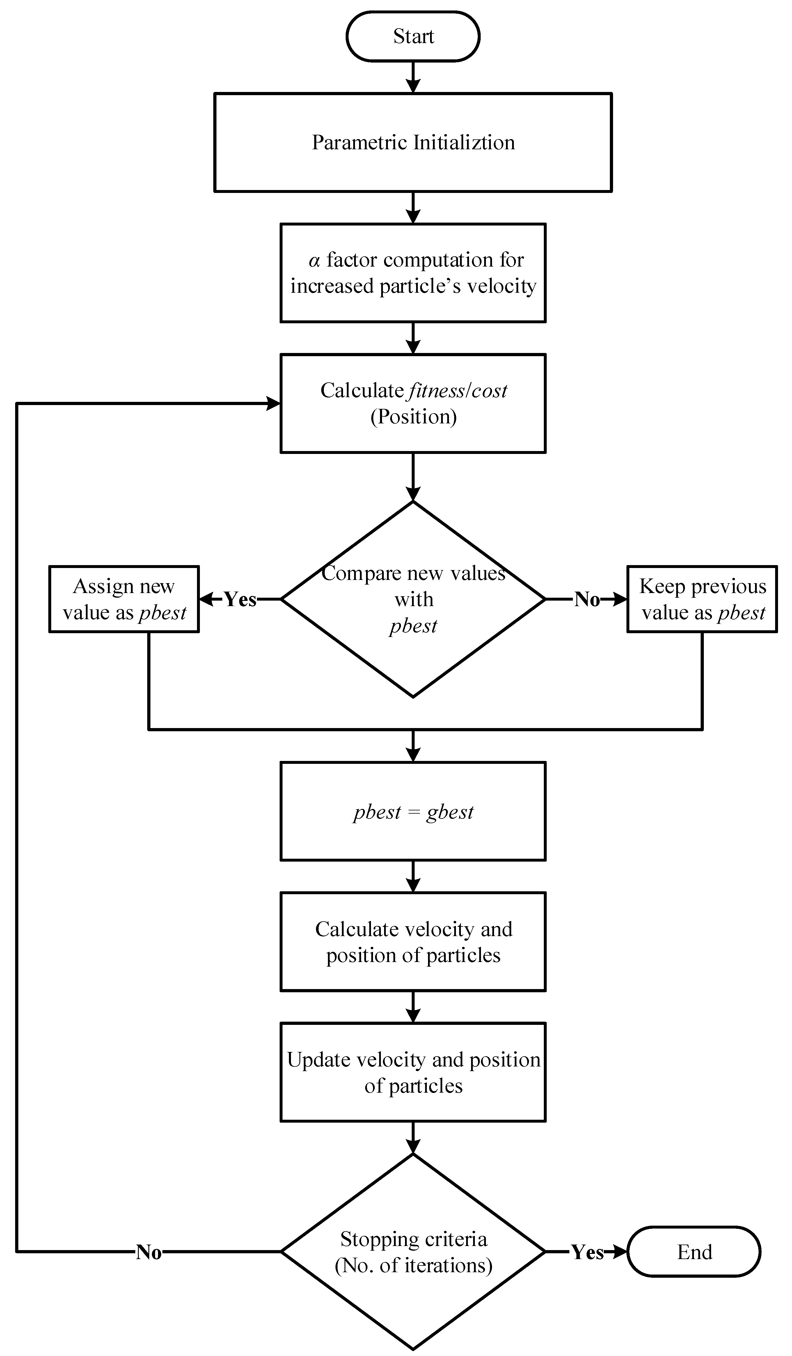
4.5. Modifications in HPSOBA

Relating to the modification of the HPSOBA, the mechanism designed is of MHPSO-BAAC with and without the constriction factor χ. The variable α is used to regulate both the social and cognitive components and accelerate the particles. Hence, in the modified algorithms presented, the velocity formulas become [19]:

$$v_{id}^{t+1}=\{\begin{array}{l}\omega v_{id}^t+\alpha ·\left((pbes{t}_{id}-x_{id}^t) +(gbes{t}_{gd}-x_{id}^t)\right)\\ \left(\omega v_{id}^t+\alpha ·\left((pbes{t}_{id}-x_{id}^t) +(gbes{t}_{gd}-x_{id}^t)\right)\right)\times \chi \end{array},$$

(14)

where the constriction factor is computed using (15),

$$\chi =\frac{2}{\left|2-\phi -\sqrt{{\phi }^2-4\phi }\right|},4.1\le \phi \le 4.2.$$

(15)

The computation of the position of the particle, and the parameters α and ω are obtained by the equations given in (11)–(13). The flow chart and pseudocode for the MHPSO-BAAC are presented in Figure 6 and Algorithm 2, respectively [39].

Algorithm 2. The MHPSO-BAACs Algorithms.

1: Initialize the factors: frequency, population, iterations and parameters

2: Initialize the velocity and position

3: for i = 1:population

4:         set velocity and position

5:         Update personal and global best values

6:                  if finest velocity < finest result of velocity

7:                            Velocity = finest result;

8:                  end if

9: end for

10: Main loop of MHPSO-BAAC and MHPSO-BAAC-χ:

11: for iteration = 1:maxit

12:         for i = 1:population

13:                  Calculate α and ω

14:                  Update position and velocity

15:                  Update personal best:

16:                  if finest velocity > velocity

17:                               position = finest position;

18:                               velocity = finest velocity;

19:                               output = finest output;

20:                          Update global best

21:                  if finest results of velocity > finest velocity

22:                               finest result = finest velocity

23:                  end if

24:                  end if

25:         end for

26: Best Cost = Best solution cost;

27: Display (iteration, Optimal Solution);

28: end for

29: Plot results

5. Working of Proposed System Model

NNs have been implemented for the forecasting of wind resources with many different approaches, including the training of the NNs through metaheuristic optimization techniques. Some recent and prominent research have been briefly discussed in the literature. The problem with using standard optimization algorithms for NN training is that wind forecasting is a completely local phenomenon, as the climatic conditions of every region of the world are different. In addition, the historical data of a region given as input values are also different for every region. Thus, in this case, generalization is not possible. However, the inherent flexibility of the NNs allows the systems to be trained and tuned according to regional requirements.

This paper presents the wind speed and power forecasting performed through the FFNN and CFNN trained through the novel HPSOBA, MHPSO-BAAC and MHPSO-BAAC optimization techniques. Historical data values for NN training play an important role in forecast efficiency. If a large number of values from past observations are considered, the NNs will become too general, and if a small number of previous observations are used for the training process, the NN will become too explicit according to those data. These situations will avoid the need to adjust according to new situations outside the data range considered. 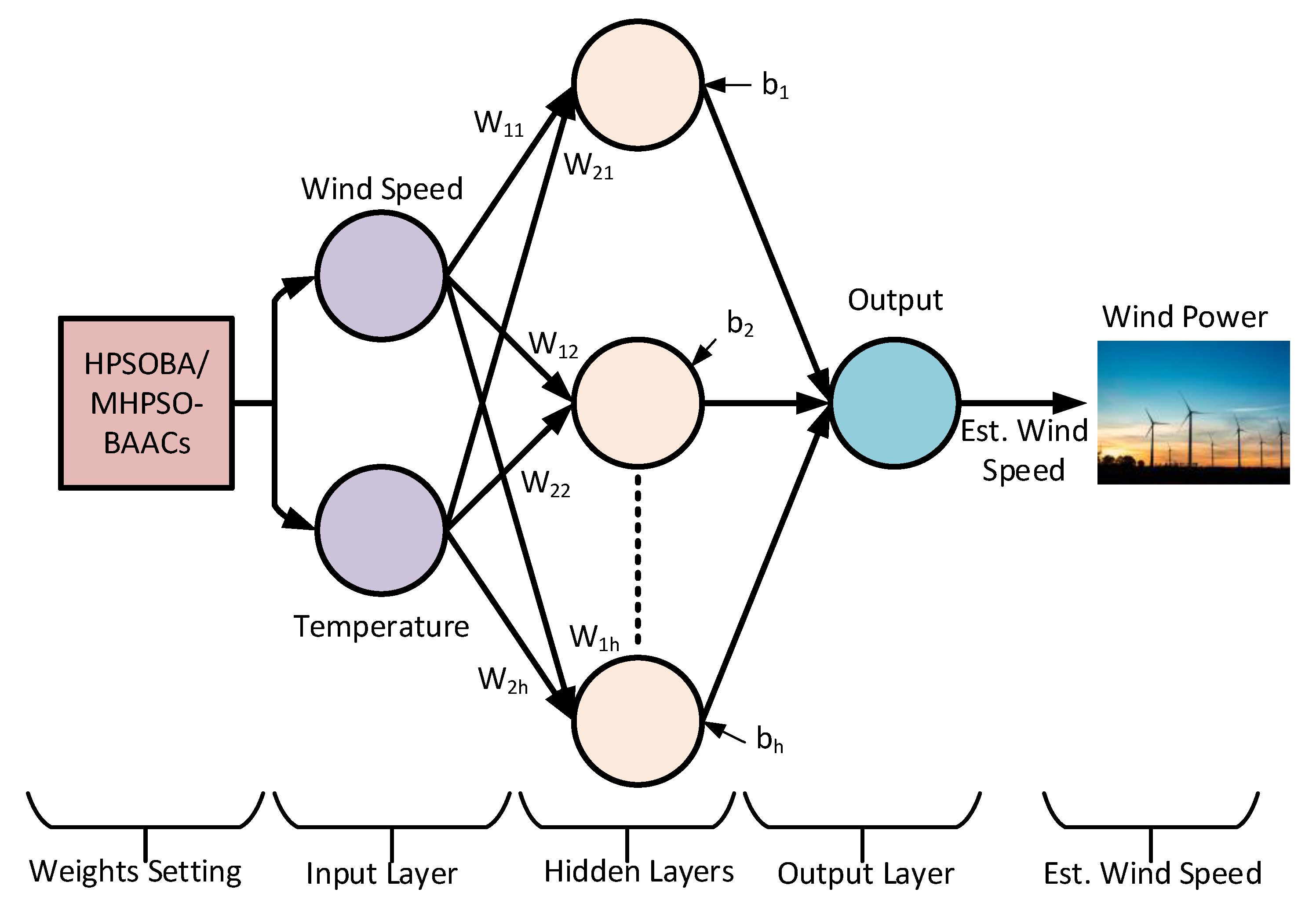Figure 7 presents the block diagram of the trained FFNN having input, output, and hidden layers.

The hidden layer consists of 150 units/neurons that are placed in parallel. The historical data for the first five months of 2019 is given to the first (input) layer of the NN. These data are processed by the NN after being trained by the mentioned optimization techniques, then the processed results are forwarded to the output layer of the NN. Overfitting is a scenario in which the algorithm tries excessively to follow the input data, resulting in its memorization. Hence, the prediction produces ambiguous results. This problem of overfitting is avoided by having a minimum number of input parameters. Thus, the input data remains simplified, and the possibility of overfitting of the target data is greatly avoided.

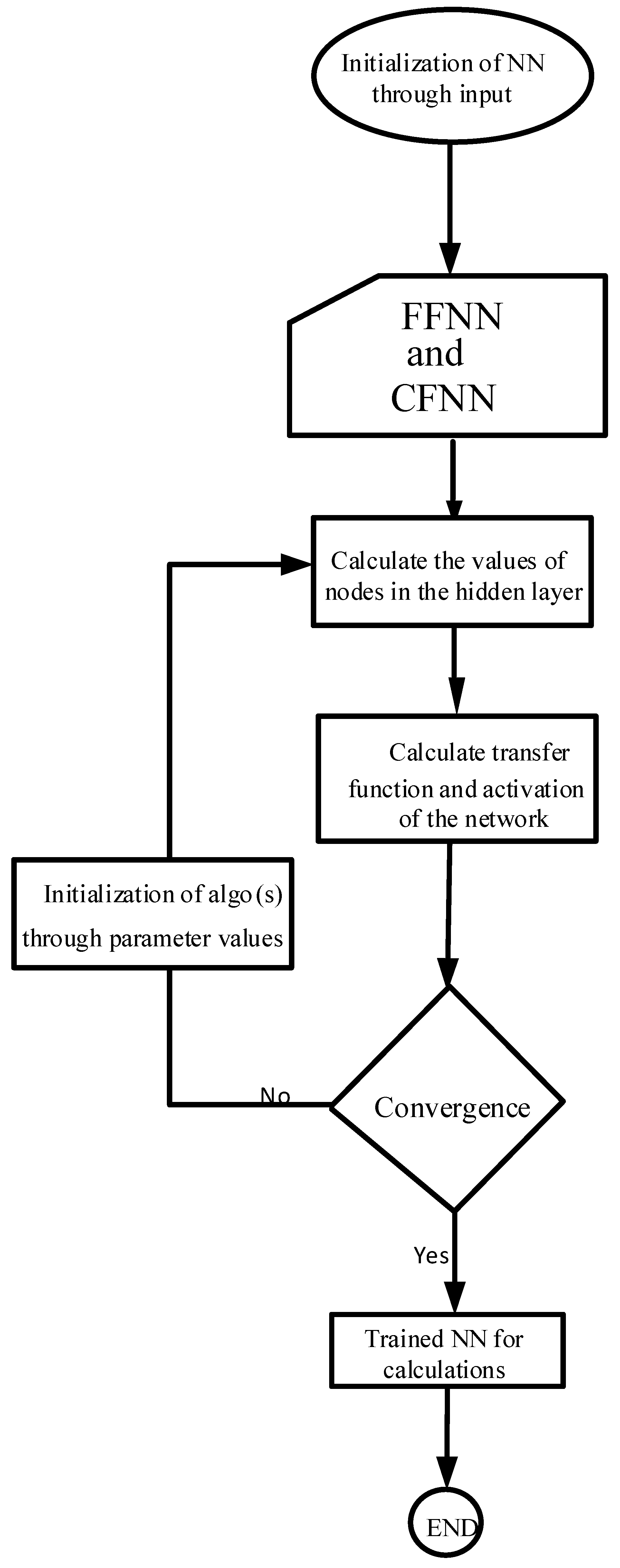
The accuracy of this output is then computed through the error calculation technique, namely MAE, MAPE and RMSE. The pictorial elaboration of the working of this system is given in the flow chart in Figure 8.

The real values of the wind speed for the next five months of 2019 are used for the accuracy determination using the Equation (5). Algorithm 3 gives the pseudocode of the algorithms used for training the FFNN and CFNN.

Algorithm 3. FFNN Trained Through HPSOBA and MHPSO-BAACs Algorithm.

1: Initialize Neural Network (FFNN or CFNN)

2: Initialize node weight and bias

3: Define objective function

4: Feed historical data as input values

5: Parameter initialization: max. iterations maxit, population npop, frequency f, ω, c and r for all algorithms

6: Set the wind velocity and position

7: for i = 1:npop

8: Initialize velocity and position

9: Update personal and global best

10: if optimum velocity < optimum result of wind velocity

11:       velocity = optimum result;

12: end if

13: end for

14: HPSOBA, MHPSO-BAAC and MHPSO-BAAC-χ main loop:

15: for iteration = 1: Maxit

16: for i = 1:npop

17: Calculate ω and α for all algorithms and χ for MHPSO-BAAC-χ only

18: Update velocity and position

19: Update personal best:

20: if velocity < optimum velocity

21: optimum position = position;

22: optimum velocity = velocity;

23: optimum output = output;

24:      Update global best

25: if optimum velocity < optimum result of wind velocity

26: optimum result = optimum velocity;

27: end if

28: end if

29: end for

30: Optimum Value = Optimal solution;

31: Display (Iteration, Optimal Solution);

32: end for

33: Check accuracy of results through error computations

34: Plot forecasted wind speed and power

6. Results and Discussion

The forecasting of the wind speed and power is performed through the FFNN trained by the standard PSO and recently designed HPSOBA, and MHPSO-BAACs algorithms to present a RES-based sustainable solution to the energy demand. Pakistan has great potential for wind-energy-based power generation, as assessed in detail by the authors in [40,41], and requires major movement for the RES-based approach as adopted by developed countries in the European Union (EU) for a smart-energy approach [42]. Although it has great potential for wind energy, the country has focused on TPPs to satisfy electric power requirements due to its variability. This emphasizes the adoption of mechanisms that make wind energy sources more reliable, especially considering the treatment of the ecosystem.

For this purpose, the algorithms have been implemented for the Jhimpir district in southern Pakistan. The district has great potential for wind energy. According to a report released by the AEDB, the region has two wind power plants with a collective installed volume of 106 MW, which is hardly 20% of the actual wind potential for the region [43]. The time resolution for the wind speed data was based on daily minimum and maximum climatic data, taken through the devices installed at various points of the wind farm and recorded for the different values of the day. The daily average wind speed and temperature were calculated and saved for 2019 [44]. The details of the considered wind farm are taken from [45] and are mentioned in

Table A1. Description of the Considered Wind Farm [46].

Sr. No.	Parameters	Values Set
1	Wind Plant Rating	49.5 MW
2	No. of Turbines	31
3	Wind Turbine Rating	1.6 MW
4	Air Density (p)	1.225 kg/m3
5	Performance Coefficient (Cp)	1
6	Wind Speed (v)	Available and Predicted Values (m/s)
7	Swept Area (A)	5346 m2
8	Hub Height	80 m

of the Appendix A section. It is worth mentioning here that the wind speed data, used for generating the forecasted results, is taken on a daily basis and spanned over the period of months. This shows that the presented results in the following subsections are for long-term forecasting derived through medium-term forecasting data, i.e., months of data derived through days of data.

The simulation performed using MATLAB^® has numerous features stated in [46]. The system on which simulation was performed is comprised of a fifth-generation AMD A-8 processor, 4 GB RAM, and a storage of 128 GB [47]. The accuracy of the predicted values is tested by the error computational techniques of MAE, MAPE, and RMSE, along with checks of the fitting of the forecasted values compared to the actual values. The details of a considered wind power generation system have been shared in the Table A1 given in the Appendix A section of the paper. The values of the simulation parameters are specified in

Table 1. Parameters of HPSOBA, MHPSO-BAACs used for simulation.

Sr. No.	Parameters	Range	Values Set
1	Inertia Weight	[0–1]	ωmin = 0.6, ωmax = 0.8
2	Cognitive and Social co-efficient	[0–4]	2.5
3	Uniform random PDF	[0–1]	0.5
4	Frequency	[0–4]	fmin = 3.0, fmax = 3.25
5	Phi	[4.1 ≤ φ ≤ 4.2]	φ = 4.1
6	Population	-	100
7	Iterations	-	1000

.

6.1. Wind Speed and Power Estimation through FFNN

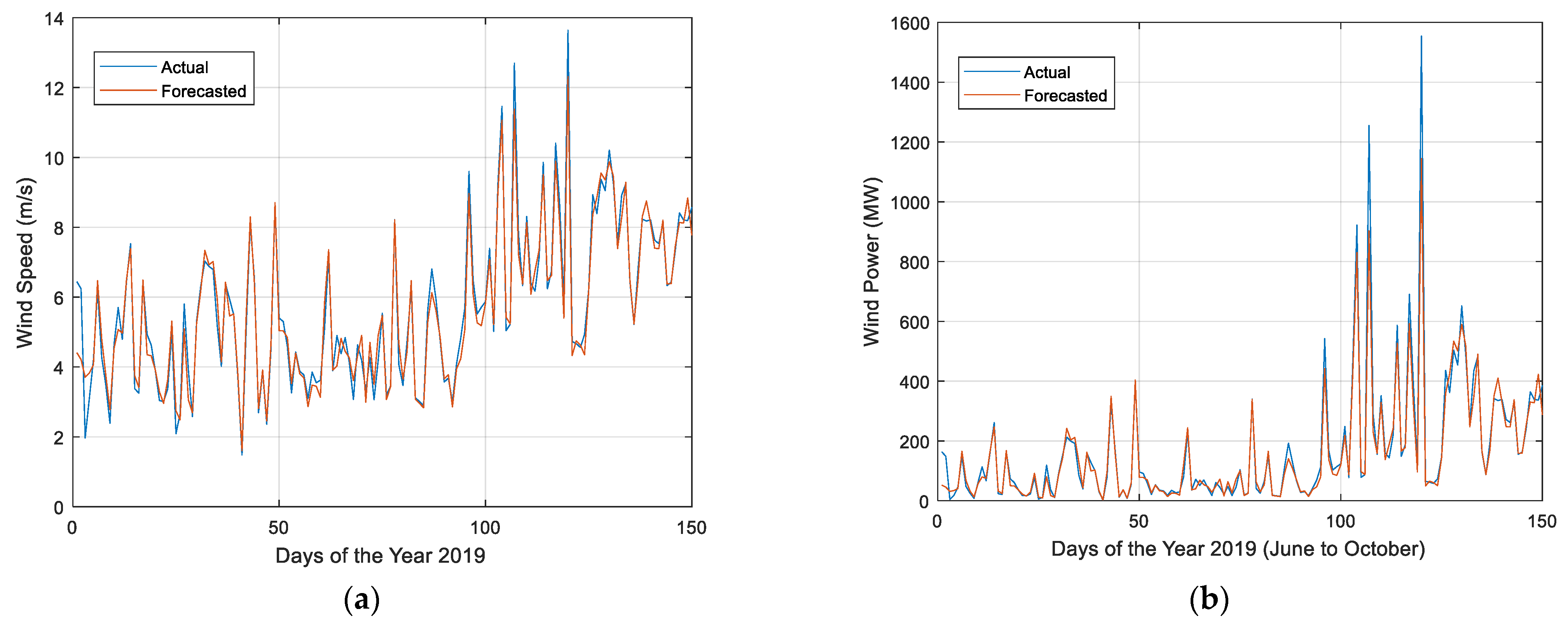
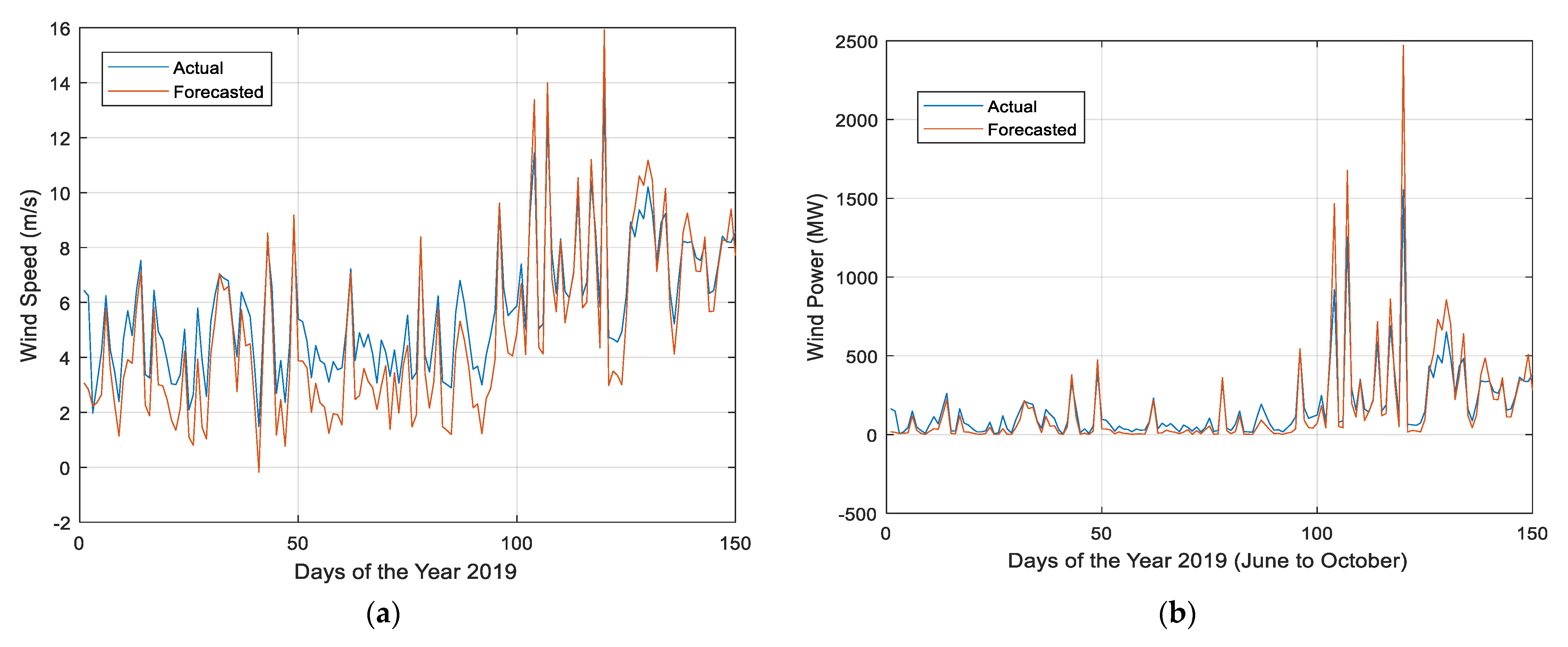
The meteorological data such as wind speed and ambient temperature for the one and half years (January 2018 to May 2019) are taken from [45,48]. The data are utilized as 150 input samples of wind speed values for one and half years, and used to predict the daily wind speed for the months of June to October 2019. The number of neurons is set to 350 with the number of inputs, hidden, and output layers set as 1 each. The weight of the neurons depends on the best-achieved values of the particles of the algorithms used to train the FFNN. The comparative wind speed and power plots for the FFNN are given in Figure 9a,b, Figure 10a,b, Figure 11a,b and Figure 12a,b, trained through standard, HPSOBA, MHPSO-BAACs algorithms, and PSO, respectively.

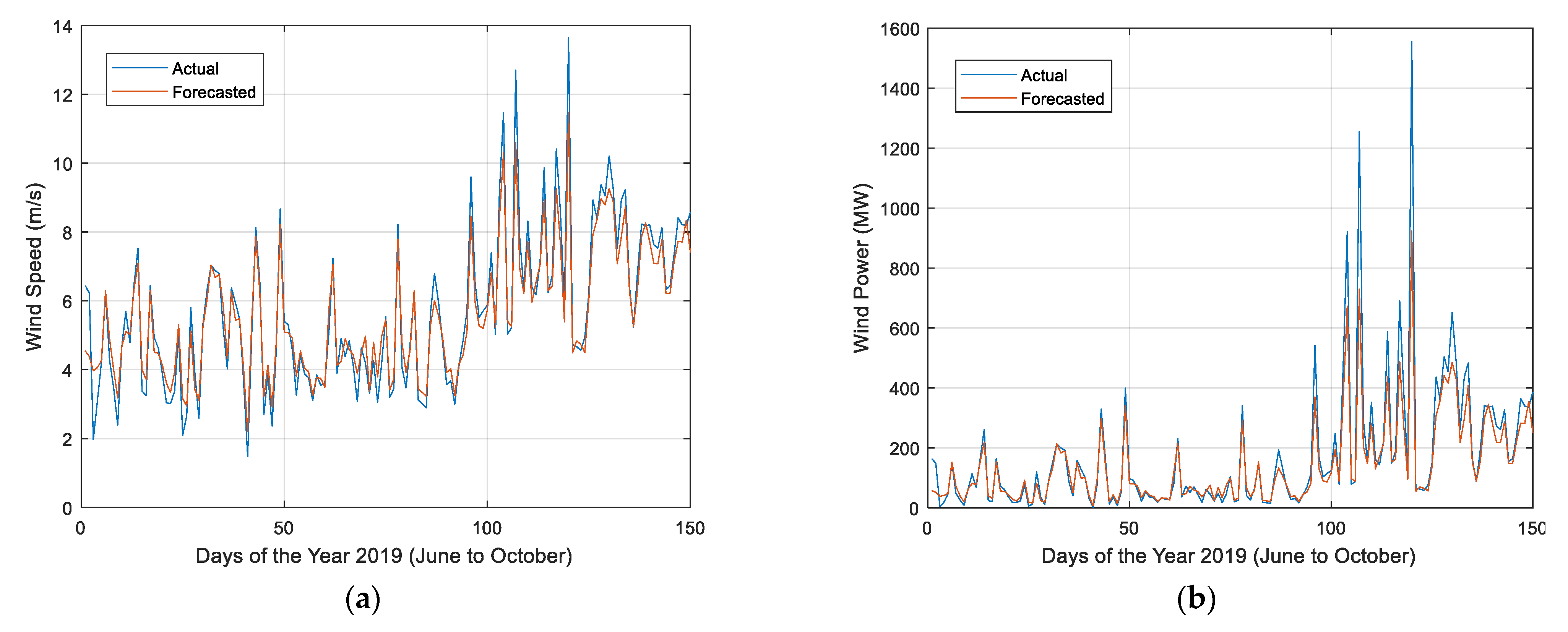
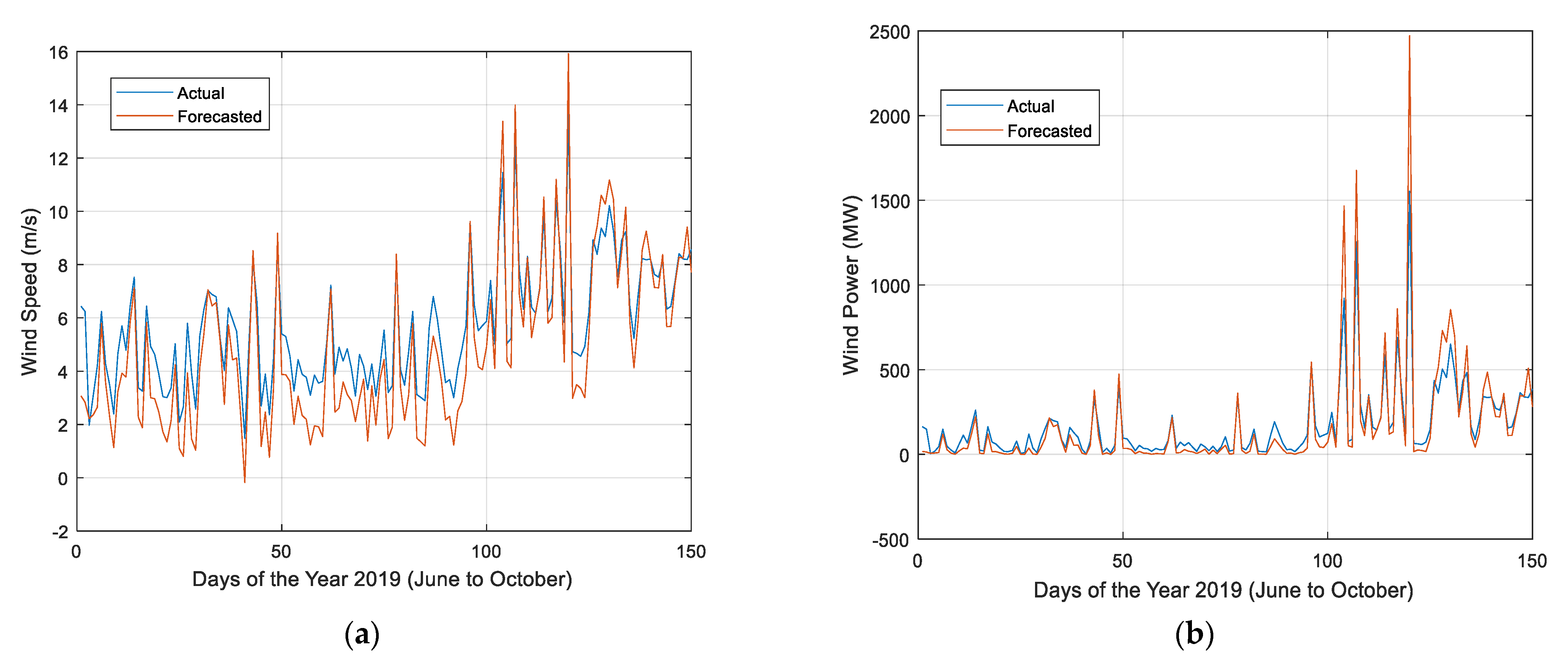
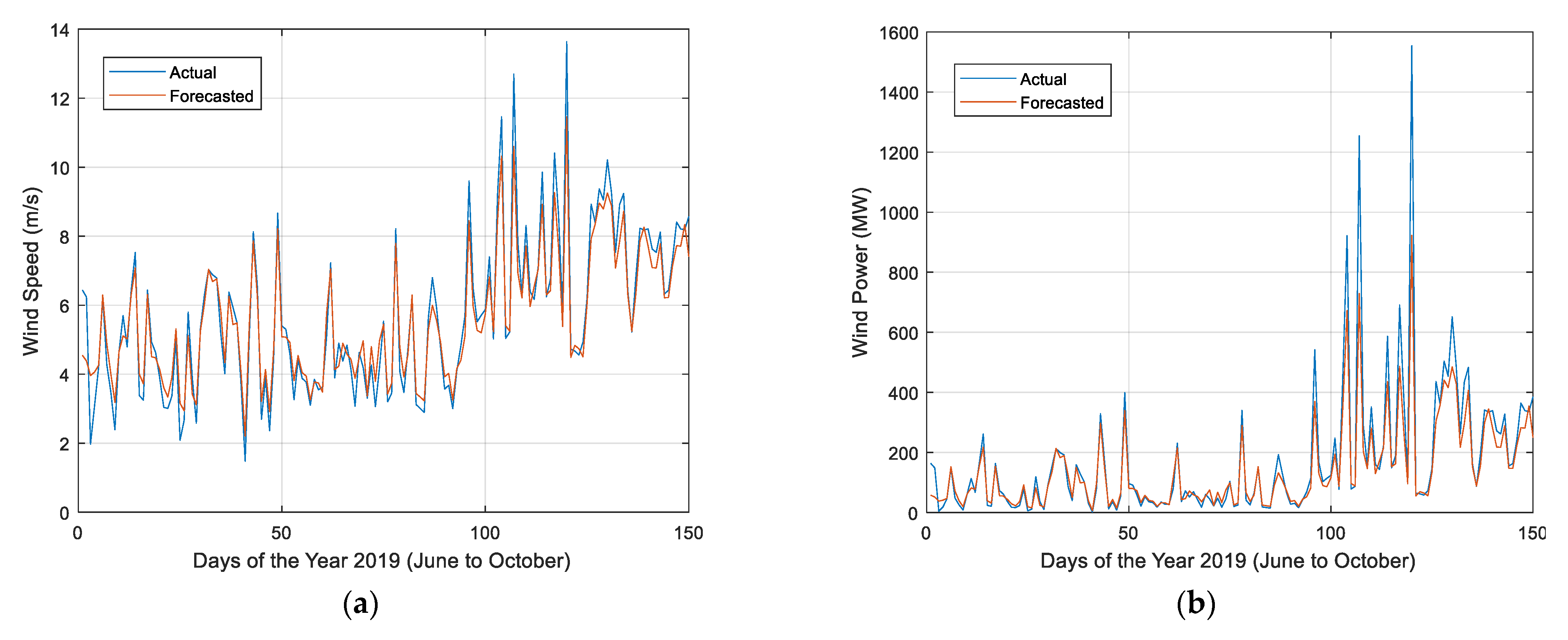
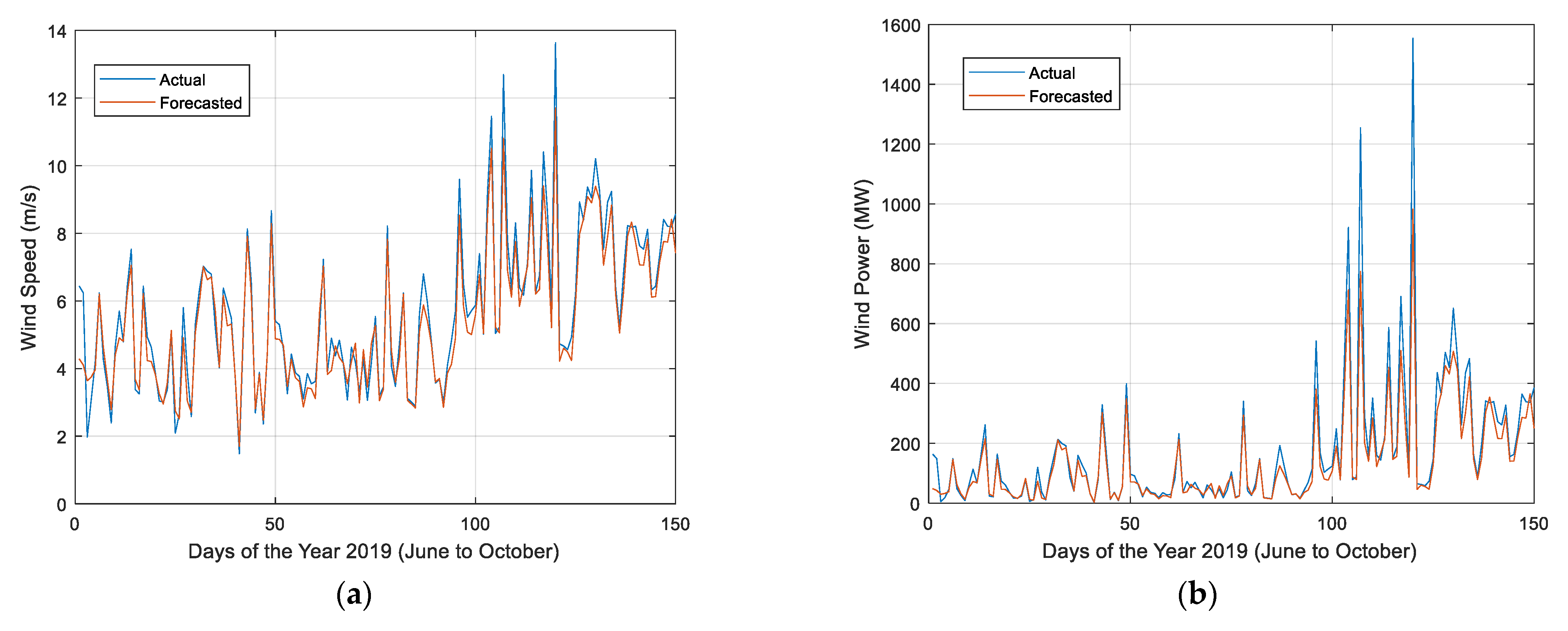
From Figure 9a, Figure 10a, Figure 11a and Figure 12a, it is evident that the FFNN trained through HPSOBA and MHPSO-BAAC provide a better wind speed forecasting that is closer to the actual values of wind speed for the same period. Figure 9b, Figure 10b, Figure 11b and Figure 12b give the comparative graphs of the wind power calculated by Equation (3) for the actual and forecast wind speed values, while the performance coefficient and the swept area are taken as 1. The figures follow the same trend, as the forecast wind power achieved by the implementation of HPSOBA and MHPSO-BAAC is closer to the actual wind power for June to October 2019, while the performance of the classical PSO appears to be a poor performer in this regard. The problem of overfitting or underfitting is avoided through a minimum number of input parameters and the required layers. Thus, the input data remains simplified and the possibility of overfitting of the target data is greatly avoided.

A similar trend is observed in the accuracy-testing procedure, performed through the calculation of the MAE, and is given in

Table 2. Values of the mean forecasted wind speed, power, and accuracy testing parameter through FFNN.

Training Techniques	Objective Function	Mean Forecasted Wind Speed (m/s)	Mean Forecasted Wind Power (MW)	MAE	MAPE (%)	RMSE	Elapsed Time (s)
HPSOBA	0.2218	5.6186	158.4656	0.0673	6.73	0.0378	64.755386
MHPSO-BAAC	0.2545	5.8107	167.0027	0.0737	7.37	0.0936	73.470082
MHPSO-BAAC-χ	0.3635	5.5867	142.6933	0.0895	8.95	0.1785	69.108956
PSO	0.3290	5.4169	138.9516	0.0876	8.76	0.5542	73.763235

.

Table 2 presents the calculated values of the objective function, MAE, MAPR, and RMSE, along with the mean estimated wind speed and power using the FFNN trained by the mentioned algorithms. Table 2 clearly shows that the superior performance in terms of the lower objective function and the error values of the designed HPSOBA and MHPSO-BAAC algorithms compared to the standard PSO. Although MHPSO-BAAC-χ shows comparatively higher error values, the mean forecasted wind power is much lower and more closely related to the actual wind power.

6.2. Wind Speed and Power Estimation through the CFNN

The algorithm compares the predicted results with 150 target samples that are from the second half of the year 2019 as mentioned above. The number of neurons is set to 350 with the number of inputs, hidden, and output layers set as 1 each. The weight of the neurons depends on the best-achieved values of the particles from the algorithms used to train the CFNN. The comparative wind speed and power graphs, along with the regression fitting graph for the CFNN are given in Figure 13a,b, Figure 14a,b, Figure 15a,b and Figure 16a,b, with the CFNN trained through the MHPSO-BAAC, MHPSO-BAAC-χ, HPSOBA, and standard PSO, respectively.

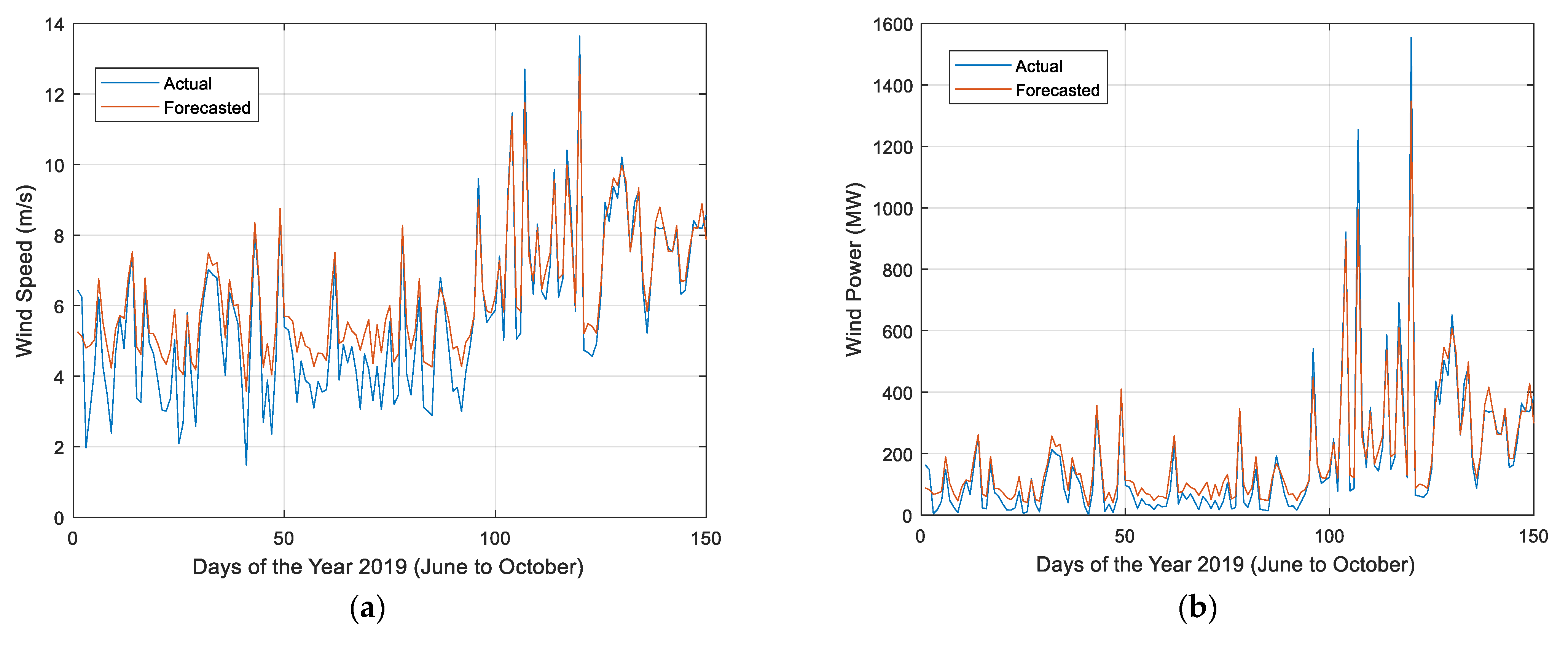
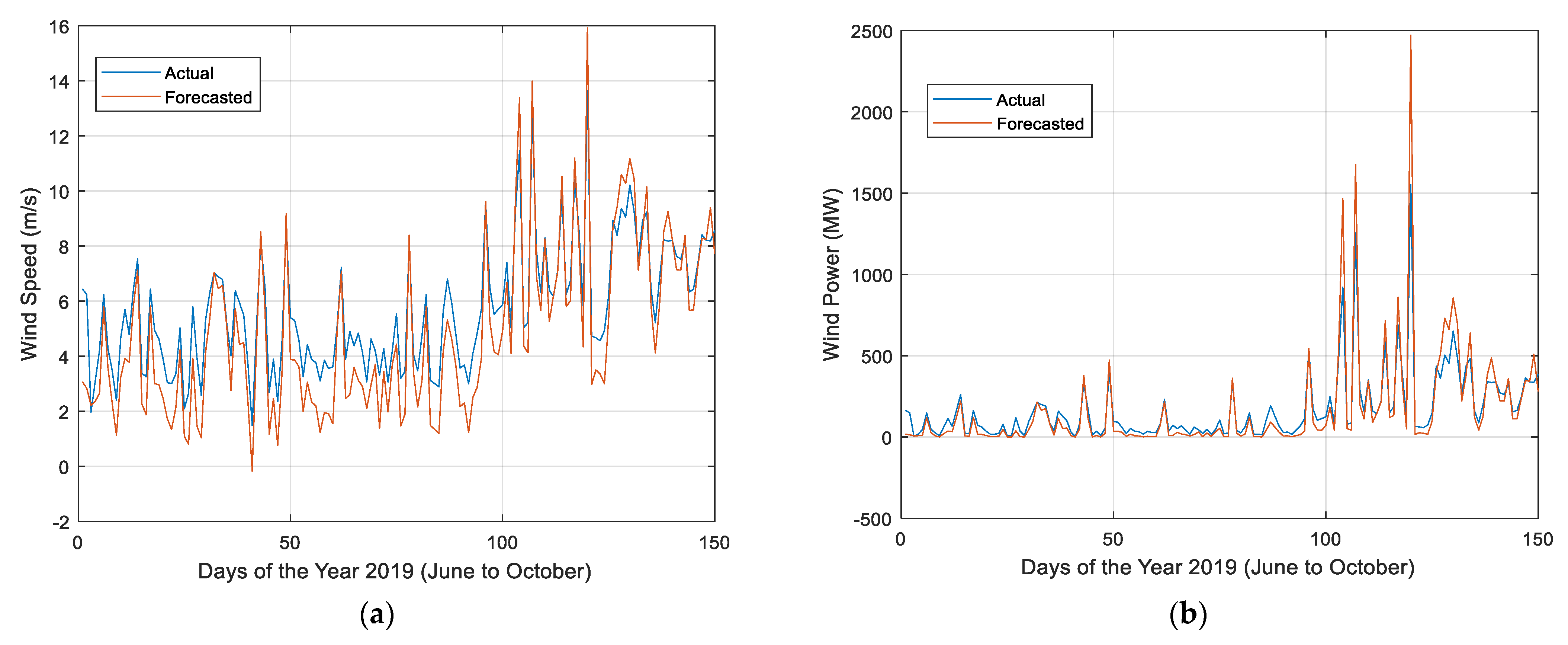
From Figure 13a, Figure 14a, Figure 15a and Figure 16a, it is evident that the CFNNs trained through the MHPSO-BAAC and MHPSO-BAAC-χ provide a good trend following the actual values of wind speed for the same period. However, the HPSOBA shows a much closer trend followed by a wind speed estimation. Figure 13b, Figure 14b, Figure 15b and Figure 16b give the comparative plots of the wind power calculated by Equation (5) for the actual and forecasted wind speed values, while the performance coefficient and the swept area are taken as one. The figures follow the same trend, as the forecasted wind power of Figure 9b, Figure 10b, Figure 11b and Figure 12b are closer to the actual wind power for June to October 2019 with the HPSOBA showing a much closer matching, while the performance by the classical PSO appears to be poor in this regard. The problem of over- and underfitting is avoided through a minimum number of input parameters and the required layers. Thus, the input data remains simplified, and the possibility of overfitting of the target data is greatly avoided.

An identical trend is observed in the accuracy-testing procedure, performed through the error value calculations, and is given in

Table 3. Values of the mean forecasted wind speed, power, and accuracy-Testing parameter through the CFNN.

Training Technique	Objective Function	Mean Forecasted Wind Speed (m/s)	Mean Forecasted Wind Power (MW)	MAE	MAPE (%)	RMSE	Elapsed Time (s)
HPSOBA	0.2780	5.2388	161.4206	0.0210	2.11	0.2347	87.243028
MHPSO-BAAC	0.2480	5.3828	167.1207	0.0112	1.12	0.0577	105.136166
MHPSO-BAAC-χ	0.3542	5.6785	146.2933	0.0895	8.95	0.2171	88.137496
PSO	0.6022	4.8238	164.1206	0.0876	8.76	0.3534	85.756344

.

Table 3 presents the calculated values of the objective function, MAE, MAPE, and RMSE, along with the mean estimated wind speed and power using the CFNN trained by the mentioned algorithms and in the time elapsed. Table 3 shows the superior performance with the lower value of the objective function, along with the error values of the MHPSO-BAAC designed of the algorithm compared to the PSO and HPSOBA, and MHPSO-BAAC-χ in the case of the MAE.

The performance comparison of both considered NNs clearly shows that the FFNN presents better results for similar training techniques and the input parameter and values. The obtained results can help in improving the contribution of wind-based power production networks in developing countries such as Pakistan that are still behind in terms of its employment, despite having huge potential. This enhanced integration can provide inexpensive electric power in the system and can reduce emissions, resulting in improved environmental conditions.

7. Conclusions and Future Work

The forecasting of wind power is a challenging task; the accurate modeling of wind speed and its generated power is intermittent as it is highly dependent on the weather, location, season, etc. Therefore, machine learning and deep learning algorithms that work on historical datasets are used in the forecasting of wind power generation.

The paper presents the forecasting of wind speed and power using FFNNs and CFNNs trained through a HPSOBA, MHPSO-BAAC, MHPSO-BAAC-χ, and PSO for June to October 2019 in the Jhimpir region in Sindh, Pakistan. Historical data from the one and half years (January 2018 to May 2019) is provided as input to the multilayer NN. The performance is analyzed through the assessment of forecasted wind speed and power against the actual values in the same period, and accuracy-testing error computational techniques using the MAE, MAPE, and RMSE. The analysis considers the comparison of the performance of the training techniques, where the HPSOBA outperforms the other training algorithms, followed by the MHPSO-BAAC. However, the overall comparative analysis validates the superior performance of the designed metaheuristic optimization algorithms of HPSOBA and MHPSO-BAACs for the forecasting mechanisms. Thus, the versatility, flexibility, and applicability of the developed algorithms is justified. The presented system predicts the daily wind speed for the mentioned period of months. As aforementioned, the presented work in this paper provides wind speed forecasting which helps in creating awareness among the government and private authorities where the location of wind-based power farms is more suitable. This will eventually result in efficient power generation, therefore a better energy output and the saving of costs. Due to the mentioned reasons, this work also acts as a guideline for the adoption of such technologies for wind-based efficient power production in developing countries that have similar climatic conditions such as the considered region in this paper. Another indirect benefit of installing this type of project is the reduction of carbon emissions in the environment. The presented work, if implemented, can help in identifying and calculating the design parameters of wind turbines for a suitable region. Furthermore, at the operational stage of the wind turbine, it can help identify the amount of electric power that can be collected from wind-based system during a particular period, hence optimizing the scheduling of the grid and reducing the operational costs of power plants by lowering the reserve capacity demand.

For future research, this model can be extended with a larger data set as training data and more accurate and long-term forecasting can also be made. The authors also plan to perform wind speed predictions using the BPNN, LSTM, and N-beats, with possible implementation of the presented optimization techniques for the training of the considered NNs, with emphasis on interpretable wind speed prediction. Wind speed modelling with interpretable physics-informed machine learning, multivariate time series, and temporal fusion transformers can be explored and evaluated with the results of this study.

References

- Hansen, J.; Kharecha, P.; Sato, M.; Masson-Delmotte, V.; Ackerman, F.; Beerling, D.J.; Hearty, P.J.; Hoegh-Guldberg, O.; Hsu, S.-L.; Parmesan, C.; et al. Assessing “Dangerous Climate Change”: Required Reduction of Carbon Emissions to Protect Young People, Future Generations and Nature. PLoS ONE 2013, 8, e81648. [Google Scholar] [CrossRef]
- Ela, E.; O’Malley, M. Studying the Variability and Uncertainty Impacts of Variable Generation at Multiple Timescales. IEEE Trans. Power Syst. 2012, 27, 1324–1333. [Google Scholar] [CrossRef]
- Widén, J.; Carpman, N.; Castellucci, V.; Lingfors, D.; Olauson, J.; Remouit, F.; Bergkvist, M.; Grabbe, M.; Waters, R. Variability Assessment and Forecasting of Renewables: A Review for Solar, Wind, Wave and Tidal Resources. Renew. Sustain. Energy Rev. 2015, 44, 356–375. [Google Scholar] [CrossRef]
- Milligan, M.; Kirby, B. Calculating Wind Integration Costs: Separating Wind Energy Value from Integration Cost Impacts; National Renewable Energy Lab.(NREL): Golden, CO, USA, 2009; p. NREL/TP-550-46275, 962504.
- Rondina, J.M.; Neto, L.M.; Alves, M.B. Technology Alternative for Enabling Distributed Generation. IEEE Lat. Am. Trans. 2016, 14, 4089–4096. [Google Scholar] [CrossRef]
- Azad, H.B.; Mekhilef, S.; Ganapathy, V.G. Long-Term Wind Speed Forecasting and General Pattern Recognition Using Neural Networks. IEEE Trans. Sustain. Energy 2014, 5, 546–553. [Google Scholar] [CrossRef]
- van Gerven, M.; Bohte, S. Editorial: Artificial Neural Networks as Models of Neural Information Processing. Front. Comput. Neurosci. 2017, 11, 114. [Google Scholar] [CrossRef] [PubMed]
- More, A.; Deo, M.C. Forecasting Wind with Neural Networks. Mar. Struct. 2003, 16, 35–49. [Google Scholar] [CrossRef]
- Imperial College Machine Learning—Neural Networks|Nuric. Available online: https://www.doc.ic.ac.uk/~nuric/teaching/imperial-college-machine-learning-neural-networks.html (accessed on 16 June 2021).
- Nasle, A. Power Analytics Corp, assignee. Systems and Methods for Real-Time Forecasting and Predicting of Electrical Peaks and Managing the Energy, Health, Reliability, and Performance of Electrical Power Systems Based on an Artificial Adaptive Neural Network. U.S. Patent 14/575,446, 23 April 2015. [Google Scholar]
- Kadhem, A.A.; Wahab, N.I.A.; Aris, I.; Jasni, J.; Abdalla, A.N. Advanced Wind Speed Prediction Model Based on a Combination of Weibull Distribution and an Artificial Neural Network. Energies 2017, 10, 1744. [Google Scholar] [CrossRef]
- Peng, H.; Liu, F.; Yang, X. A Hybrid Strategy of Short Term Wind Power Prediction. Renew. Energy 2013, 50, 590–595. [Google Scholar] [CrossRef]
- Lv, S.-X.; Wang, L. Deep Learning Combined Wind Speed Forecasting with Hybrid Time Series Decomposition and Multi-Objective Parameter Optimization. Appl. Energy 2022, 311, 118674. [Google Scholar] [CrossRef]
- Duan, Z.; Liu, H.; Li, Y.; Nikitas, N. Time-Variant Post-Processing Method for Long-Term Numerical Wind Speed Forecasts Based on Multi-Region Recurrent Graph Network. Energy 2022, 259, 125021. [Google Scholar] [CrossRef]
- Howland, M.F.; Dabiri, J.O. Wind Farm Modeling with Interpretable Physics-Informed Machine Learning. Energies 2019, 12, 2716. [Google Scholar] [CrossRef]
- Wu, B.; Wang, L.; Zeng, Y.-R. Interpretable Wind Speed Prediction with Multivariate Time Series and Temporal Fusion Transformers. Energy 2022, 252, 123990. [Google Scholar] [CrossRef]
- Huang, C.-J.; Kuo, P.-H. A Short-Term Wind Speed Forecasting Model by Using Artificial Neural Networks with Stochastic Optimization for Renewable Energy Systems. Energies 2018, 11, 2777. [Google Scholar] [CrossRef]
- Nazaré, G.; Castro, R.; Gabriel Filho, L.R. Wind Power Forecast Using Neural Networks: Tuning with Optimization Techniques and Error Analysis. Wind Energy 2020, 23, 810–824. [Google Scholar] [CrossRef]
- Ellahi, M.; Abbas, G.; Khan, I.; Koola, P.M.; Nasir, M.; Raza, A.; Farooq, U. Recent Approaches of Forecasting and Optimal Economic Dispatch to Overcome Intermittency of Wind and Photovoltaic (PV) Systems: A Review. Energies 2019, 12, 4392. [Google Scholar] [CrossRef]
- Shabbir, N.; Kütt, L.; Jawad, M.; Husev, O.; Rehman, A.U.; Gardezi, A.A.; Shafiq, M.; Choi, J.G. Short-Term Wind Energy Forecasting Using Deep Learning-Based Predictive Analytics. CMC-Comput. Mater. Continua 2022, 72, 1017–1033. [Google Scholar] [CrossRef]
- Shabbir, N.; Ahmadiahangar, R.; Kütt, L.; Iqbal, M.N.; Rosin, A. Wind Energy Forecasting using Recurrent Neural Networks. In Proceedings of the IEEE International Conference on Big Data, Knowledge and Control Systems Engineering (BdKCSE’2019), Sofia, Bulgaria, 21–22 November 2019. [Google Scholar]
- Ellahi, M.; Abbas, G. A Hybrid Metaheuristic Approach for the Solution of Renewables-Incorporated Economic Dispatch Problems. IEEE Access 2020, 8, 127608–127621. [Google Scholar] [CrossRef]
- Ellahi, M.; Abbas, G.; Satrya, G.B.; Usman, M.R.; Gu, J. A Modified Hybrid Particle Swarm Optimization With Bat Algorithm Parameter Inspired Acceleration Coefficients for Solving Eco-Friendly and Economic Dispatch Problems. IEEE Access 2021, 9, 82169–82187. [Google Scholar] [CrossRef]
- Warsito, B.; Santoso, R.; Suparti; Yasin, H. Cascade Forward Neural Network for Time Series Prediction. J. Phys. Conf. Ser. 2018, 1025, 012097. [Google Scholar] [CrossRef]
- Bebis, G.; Georgiopoulos, M. Feed-Forward Neural Networks. IEEE Potentials 1994, 13, 27–31. [Google Scholar] [CrossRef]
- Feedforward Neural Networks—An Overview|ScienceDirect Topics. Available online: https://www.sciencedirect.com/topics/chemical-engineering/feedforward-neural-networks (accessed on 15 June 2021).
- Bañuelos-Ruedas, F.; Angeles-Camacho, C.; Rios-Marcuello, S. Methodologies Used in the Extrapolation of Wind Speed Data at Different Heights and Its Impact in the Wind Energy Resource Assessment in a Region. Wind Farm-Tech. Regul. Potential Estim. Siting Assess. 2011, 97, 114. [Google Scholar] [CrossRef]
- Jiang, Y.; Song, Z.; Kusiak, A. Very Short-Term Wind Speed Forecasting with Bayesian Structural Break Model. Renew. Energy 2013, 50, 637–647. [Google Scholar] [CrossRef]
- Houssein, E.H. Particle Swarm Optimization-Enhanced Twin Support Vector Regression for Wind Speed Forecasting. J. Intell. Syst. 2017, 28, 905–914. [Google Scholar] [CrossRef]
- Catalao, J.P.S.; Pousinho, H.M.I.; Mendes, V.M.F. An Artificial Neural Network Approach for Short-Term Wind Power Forecasting in Portugal. In Proceedings of the 2009 15th International Conference on Intelligent System Applications to Power Systems, Curitiba, Brazil, 8–12 November 2009; pp. 1–5. [Google Scholar]
- Liu, Z.; Gao, W.; Wan, Y.-H.; Muljadi, E. Wind Power Plant Prediction by Using Neural Networks. In Proceedings of the 2012 IEEE Energy Conversion Congress and Exposition (ECCE), Raleigh, NC, USA, 15–20 September 2012; pp. 3154–3160. [Google Scholar]
- Monfared, M.; Rastegar, H.; Kojabadi, H.M. A New Strategy for Wind Speed Forecasting Using Artificial Intelligent Methods. Renew. Energy 2009, 34, 845–848. [Google Scholar] [CrossRef]
- Ren, C.; An, N.; Wang, J.; Li, L.; Hu, B.; Shang, D. Optimal Parameters Selection for BP Neural Network Based on Particle Swarm Optimization: A Case Study of Wind Speed Forecasting. Knowl.-Based Syst. 2014, 56, 226–239. [Google Scholar] [CrossRef]
- Wang, J.; Zhou, Q.; Jiang, H.; Hou, R. Short-Term Wind Speed Forecasting Using Support Vector Regression Optimized by Cuckoo Optimization Algorithm. Available online: https://www.hindawi.com/journals/mpe/2015/619178/ (accessed on 2 September 2020).
- Imran, M.; Hashim, R.; Khalid, N.E.A. An Overview of Particle Swarm Optimization Variants. Procedia Eng. 2013, 53, 491–496. [Google Scholar] [CrossRef]
- Abbas, G.; Gu, J.; Farooq, U.; Asad, M.U.; El-Hawary, M. Solution of an Economic Dispatch Problem Through Particle Swarm Optimization: A Detailed Survey—Part I. IEEE Access 2017, 5, 15105–15141. [Google Scholar] [CrossRef]
- Abbas, G.; Gu, J.; Farooq, U.; Raza, A.; Asad, M.U.; El-Hawary, M.E. Solution of an Economic Dispatch Problem Through Particle Swarm Optimization: A Detailed Survey—Part II. IEEE Access 2017, 5, 24426–24445. [Google Scholar] [CrossRef]
- Zhang, J.-M.; Xie, L. Particle Swarm Optimization Algorithm for Constrained Problems. Asia-Pac. J. Chem. Eng. 2009, 4, 437–442. [Google Scholar] [CrossRef]
- Shi, Y.; Eberhart, R. A Modified Particle Swarm Optimizer. In Proceedings of the 1998 IEEE International Conference on Evolutionary Computation Proceedings. IEEE World Congress on Computational Intelligence (Cat. No.98TH8360), Anchorage, AK, USA, 4–9 May 1998; pp. 69–73. [Google Scholar]
- Shami, S.H.; Ahmad, J.; Zafar, R.; Haris, M.; Bashir, S. Evaluating Wind Energy Potential in Pakistan’s Three Provinces, with Proposal for Integration into National Power Grid. Renew. Sustain. Energy Rev. 2016, 53, 408–421. [Google Scholar] [CrossRef]
- Ghafoor, A.; ur Rehman, T.; Munir, A.; Ahmad, M.; Iqbal, M. Current Status and Overview of Renewable Energy Potential in Pakistan for Continuous Energy Sustainability. Renew. Sustain. Energy Rev. 2016, 60, 1332–1342. [Google Scholar] [CrossRef]
- Islands “Smart Energy” for Eco-Sustainable Energy a Case Study “Favignana Island” | IIETA. Available online: http://iieta.org/journals/ijht/paper/10.18280/ijht.35Sp0112 (accessed on 23 December 2020).
- Data Collection Survey on Renewable Energy Development in Pakistan: Final Report. Available online: https://openjicareport.jica.go.jp/643/643/643_117_12086740.html (accessed on 24 June 2021).
- Ullah, Z.; Ali, S.M.; Khan, I.; Wahab, F.; Ellahi, M.; Khan, B. Major Prospects of Wind Energy in Pakistan. In Proceedings of the 2020 International Conference on Engineering and Emerging Technologies (ICEET), Lahore, Pakistan, 22–23 February 2020; pp. 1–6. [Google Scholar]
- Jhimpir Weather Forecast. Available online: https://www.worldweatheronline.com/jhimpir-weather/sindh/pk.aspx (accessed on 2 September 2020).
- Application of Jhimpir.Pdf. Available online: https://nepra.org.pk/licensing/Licences/Licence%20Application/2014/July%202014/Application%20of%20Jhimpir.pdf (accessed on 2 September 2020).
- Symbolic Math Toolbox—MATLAB. Available online: https://www.mathworks.com/products/symbolic.html (accessed on 2 September 2020).
- Jhimpir Monthly Climate Averages. Available online: https://www.worldweatheronline.com/jhimpir-weather/sindh/pk.aspx (accessed on 2 December 2020).
Figure 1.
Block diagram of the presented system.
Figure 2.
The architecture of the feedforward neural network (FFNN) [
24,
26,
33].
Figure 3.
The architecture of the cascade forward neural Network (CFNN) [
24].
Figure 4.
PSO’s pictorial description.
Figure 5.
Flow chart of the HPSOBA.
Figure 6.
Flow Chart of the MHPSO-BAACs.
Figure 7.
Block Diagram of Trained Neural Networks.
Figure 8.
Flow Chart of NNs trained through HPSOBA, MHPSO-BAACs, and PSO.
Figure 9.
(a) Comparative analysis of wind speed forecasting by the FFNN trained through HPSOBA. (b) Comparative analysis of wind power forecasting by the FFNN trained through HPSOBA.
Figure 10.
(a) Comparative analysis of wind speed forecasting by the FFNN trained through MHPSO-BAAC. (b) Comparative analysis of aind power forecasting by the FFNN trained through MHPSO-BAAC.
Figure 11.
(a) Comparative analysis of wind speed forecasting by the FFNN trained through MHPSO-BAAC-χ. (b) Comparative analysis of wind power forecasting by the FFNN trained through MHPSO-BAAC-χ.
Figure 12.
(a) Comparative analysis of wind speed forecasting by the FFNN trained through PSO. (b) Comparative analysis of wind power forecasting by the FFNN trained through PSO.
Figure 13.
(a) Comparative analysis of wind speed forecasting by the CFNN trained through HPSOBA. (b) Comparative analysis of wind power forecasting by the CFNN trained through HPSOBA.
Figure 14.
(a) Comparative analysis of wind speed forecasting by the CFNN trained through MHPSO-BAAC. (b) Comparative analysis of wind power forecasting by the CFNN trained through MHPSO-BAAC.
Figure 15.
(a) Comparative analysis of wind speed forecasting by the CFNN trained through MHPSO-BAAC-χ. (b) Comparative analysis of wind power forecasting by the CFNN trained through MHPSO-BAAC-χ.
Figure 16.
(a) Comparative analysis of wind speed forecasting by the CFNN trained through PSO. (b) Comparative analysis of wind power forecasting by the CFNN trained through PSO.