Abstract
With the development of energy integration technology, demand response (DR) has gradually evolved into integrated demand response (IDR). In this study, for the integrated energy system (IES) on the distribution grid side with electricity, heat, natural gas network, and hydrogen energy equipment, the analogy relationship between the thermal and mobile hydrogen energy storage networks is proposed. Moreover, a unified model that reflects network commonalities across different energy forms is established. Then, considering the time delay of the IES in the nontransient network, a time-domain two-port model of the IES considering the time delay is established. This model shows the joint effect of time and space on system parameters. Finally, this study validates the model in the application of DR. The verification results show that in DR, the time-domain two-port model can accurately “cut peaks and fill valleys” for the IES and effectively reduce the operating cost of the IES system.
1. Introduction
The integrated energy system (IES) with electricity, heat, natural gas network, and hydrogen energy as the core realizes the coupling of heterogeneous energy flows and the synergy and complementarity of multienergy flows through multiple types of equipment. In addition, the IES has changed the current situation of only using electric energy to meet the needs of users for cooling, heating, and electricity. Moreover, the economic efficiency and utilization rate of the system have improved, and the IES has promoted the consumption of renewable energy, which has been widely used in production and life [1].
Many studies on the optimal operation of the IES exist. Geidl et al. [2] proposed an energy hub (EH) for the first time, which laid the foundation for subsequent scholars to study the modeling, planning, and operation of the IES. Xie et al. [3] comprehensively considered transportation, natural gas, and active distribution networks in IES modeling and promoted the intelligence of multi-energy systems. Ma et al. [4] took cogeneration and power-to-gas and carbon capture system as a whole system, and analyzed its coupling characteristics of electricity, heat, gas, and carbon. Liu et al. [5] used power flow calculation to combine cogeneration devices, heat pumps, and electric boilers and performed simple scheduling. For the IES at the community level, Wang et al. [6] proposed a two-stage collaborative optimization method considering a day-ahead optimal scheduling strategy and intraday scheduling. In recent years, the development of electric hydrogen production technology [7] can not only promote the consumption of new energy but also accelerate the electrification of energy consumption through the production of hydrogen energy equipment. With the maturity of hydrogen storage technology, the application of hydrogen energy storage is becoming increasingly extensive [8]. Recently, “Sesame Solar” has developed a mobile nanogrid powered by solar energy and green hydrogen. The green hydrogen produced by electrolysis is stored at low pressure in onboard solid hydrogen tanks, which can be easily and safely transported and fuel the onboard hydrogen fuel cells while charging the batteries. The mobile nanogrid not only is sturdy and durable but also can be moved to a suitable location to meet the needs of different application scenarios. Many similar studies in these years have also provided a good development environment for the development of hydrogen energy. However, problems still exist presently, such as unbalanced energy utilization [9] and insufficient new energy consumption [10] in the power system. Hence, we will try to embed mobile hydrogen energy storage (MHES) into the well-researched IES and will simulate the embedded system in terms of integrated demand response (IDR).
Demand response (DR) is an electricity consumption management mechanism for customers to respond to time-of-use electricity price signals or real-time scheduling instructions. In terms of practical application of electricity consumption management, Ireland exercises explicit priority dispatch of renewables [11], which can lend itself to providing consumers with day-ahead half-hourly pricing signals and can be leveraged for the DR process design in this paper. Considering that IDR is an extension of traditional power DR in the energy Internet, many scholars have made extensive explorations on IDR based on DR. Tan et al. [12] considered the asynchrony of the thermal network and power grid, and established a two-stage robust optimization model based on price-based demand response (PBDR). Zheng et al. [13] considered the coupling effects of the supply side and the demand side respectively, and proposed a two-layer IDR model based on incentives. Bahrami et al. [14] and Huang et al. [15] compared the correlation and difference between traditional power DR and IDR. Li et al. [9] considered robust stability in the IDR model, aiming to reduce the volatility of renewable energy output. He et al. [16] developed an IDR optimization framework including day-ahead and intraday stages considering multiple uncertainties. In the regional IES, gas and electricity are considered.
The above studies explored the energy management of the IES, but they only examined the IDR of the IES system from the perspective of energy balance and economic optimization on a long-term scale. Li et al. [17] referred to the power system model, established the network constraints of the natural gas system, and applied it in the IES security region, but did not pay attention to the delay effect. Ceseña et al. [18] used a two-stage model based on mixed integer linear programming to optimize the time-ahead set points of all controllable devices, but only for robust stability. Parra et al. [19] proposed that hydrogen can further integrate the traditional power, heat, and transportation sectors, which put forward new requirements for the steady-state characteristics of the IES. As a complex physical network, the power transmission in the power system follows Ohm’s law, whereas the thermal and natural gas networks follow the fluid mass and energy conservation equations [20]. This case also makes the different systems in the IES have significant differences in operating time scales. This difference will greatly affect the accuracy and effectiveness of traditional optimal scheduling strategies. In addition, no MHES has been involved in IDR research yet. To solve this problem, this current study will try to establish a unified model in the IES with electricity, natural gas network, heat, and hydrogen energy as the core and then provide a reference for IDR management.
This study has three main contributions:
(1) This study has established a universal IES architecture on the distribution network side and tried to imitate the thermal network model to establish a network model of hydrogen energy storage with mobility characteristics and then add it to a new IES dispatch architecture.
(2) Based on the multiple uncertainty factors of the system and the characteristics of energy users, a time-domain two-port IES unified model is established, which considers delays. The model can reflect the coupling and spatiotemporal relationships among multiple parties in energy supply and demand, establishing a basis for subsequent research.
(3) The study has established an IDR model of the IES with MHES, which considers the spatiotemporal characteristics of energy flow and aims to optimize the total operating cost.
2. Laplace Domain Physics Model of the IES
The IES studied in this chapter includes power, thermal, natural gas, and MHES transportation networks.
2.1. Unified Model of the IES
The analysis and scheduling of the existing IDR are generally based on the coupled model of electricity, gas, and heat established using the concept of EH [21]. Although this model can intuitively couple different forms of energy together, this coupling will bring greater computational complexity in terms of calculation. In addition, if the influence of time delay on the thermal and natural gas networks is additionally considered, rewriting the coupling model in related studies would be difficult. Notably, electricity, heat, and natural gas have many similar characteristics in energy transmission [22]: the power and heat transmissions reflect the effect of potential energy and damping on energy, and the relationship curve of natural gas pressure and flow is similar to the dynamic process of an electric resistor–capacitor circuit. For the above considerations, this section attempts to find a unified model form for different energy networks. In addition, considering that MHES has relatively independent power support functions and certain dispatchable characteristics, this section attempts to convert MHES into a form similar to the heat grid and integrate it into the IES system to provide a modeling basis for the subsequent time-domain two-port model considering time delay. The following reasonable assumptions are made for the two-port model below: (a) In the power flow, alternating current (AC) power system and power lines are uniform transmission lines. (b) In the thermal flow, the flow rate of the fluid is constant, and the static heat conduction inside the fluid is ignored. (c) In the gas flow, the temperature change and height change of the gas pipeline are ignored; the reference operating point is known; the gas-pipeline-regulating valve is not adjusted.
2.1.1. Electricity Network
The transmission of typical AC satisfies Maxwell’s equation, and it can be generally considered that the medium of the transmission line is uniform. Considering the line and transformer models comprehensively, a classic power network branch equivalent circuit diagram is established, as shown in Figure 1.
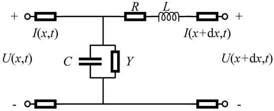
Figure 1.
Classic power network branch equivalent circuit diagram.
In Figure 1, U(x,t) and I(x,t) are the voltage and current of the power flow at position x of the transmission line at time t, respectively; R and L are the branch resistance and reactance per unit length, respectively; dx is the unit length; and Y and C are the ground admittance per unit length (excluding the ground capacitance) and the ground capacitance, respectively. As this model is the basic model on which power system analysis is well known, we can try to equate the grid, heat grid, natural gas grid, and MHES mobile network as similar network models. According to the equivalent circuit diagram (Figure 1), the mathematical equation of the power network can be expressed as Equations (1) and (2).
2.1.2. Thermal Network
Unlike the power system, thermal networks do not follow transient electromagnetic laws but follow heat migration and heat conduction processes with a time scale of minutes or hours. The heat transfer in the pipeline is expressed as the change of the water temperature at position x with time t. After ignoring the static heat conduction inside the water flow, the heat transfer equations can be expressed as follows [23]:
In Equation (3), the first two items on the left represent the convective heat transfer of the water in the supply pipe and the return pipe, and the third term represents the heat loss of the pipe. T(x,t) is the temperature difference between the water flow at position x in the pipe and the reference temperature at time t, which is a function of x and t; ρ is the density of water; m is the mass flow rate of the water flow and can be assumed to be constant; c is the specific heat capacity of water; λh is the thermal conductivity of the pipe; and S is the cross-sectional pipe area. In Equation (4), Q(x,t) represents the heat flow power. By combining the two equations, equations similar in format to the power network equations can be obtained as Equations (5) and (6), where v is the velocity of water.
2.1.3. Natural Gas Network
Isothermal natural gas is transported by pressure, and the gas flow obeys the conservation-of-mass law and Bernoulli’s law for nonideal gases. The transmission process is generally described by the continuity and momentum equations. Taking the pressure p(x,t) and the flow rate q(x,t) as the state quantities, ignoring the partial derivative term describing the change of the flow rate with time, the natural gas state equations can be expressed as Equations (7) and (8) [24]:
In Equations (7) and (8), p(x,t) is the pressure of the gas flow at pipe position x at time t, q(x,t) is the volume flow rate of the gas flow at the pipe position x at time t (m3/s, both measured under standard conditions, that is, under 1 atmospheric pressure and 25 °C), va is the speed of sound in gas, w is the average flow velocity of the gas pipeline, D is the inner diameter of the pipeline, λg is the friction coefficient of the gas pipeline, and Sg is the cross-sectional pipeline area of the natural gas branch. In addition, if the gas constant of natural gas is Rg, and the temperature of the pipeline is Tg, then the flow rate q(x,t) and pressure p(x,t) have the following relationship:
2.1.4. MHES Network
MHES is a new energy storage technology in recent years. This energy storage has the characteristics of cleanliness and high energy density and generally uses metal hydride (MH) as the energy storage matrix. The MHES model used in this study is based on [8], which pointed out that this hydrogen energy storage can be carried by small cars or even individuals and can realize the functions of existing mobile energy storage. Considering that the battery is portable, versatile, and easy to dispatch, this study can assume that the energy distribution of MHES on the transportation network is uniform and discretized, which can be defined as virtual energy storage flow (VESF). In addition, considering the cyclic use of mobile energy storage, there must be supporting charging equipment (charging stations and charging piles) and discharging equipment (user loads) in the transportation network. The two are not necessary to be in the same place. Therefore, this study can assume that the MHES network has “water supply and return pipes” similar to the thermal network. The stored energy can also be consumed when the hydrogen stored energy is transported. Notably, as MHES has the characteristics of traditional energy storage, that is, it can switch between the identity of load and power source, this research can be equivalent to MHES in two parts: (1) traditional nonmobile energy storage with the function of smoothing fluctuations and (2) electric vehicle hydrogen energy storage participating in mobile dispatching. To unify the research content, this study integrates the first part into the load and distributed generators (DG) modeling and then focuses on the second part in the following. According to the above analysis, the MHES dispatch network and thermal network have relatively consistent characteristics. This study will model and analyze the MHES network based on the above analysis. Table 1 shows the analogy process.

Table 1.
Comparison of the thermal network and the MHES network.
Figure 2 depicts a schematic diagram of the designed MHES network.
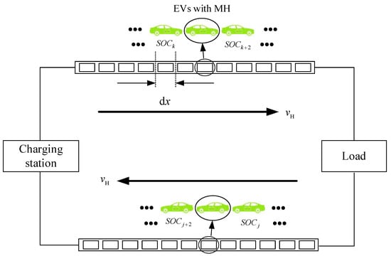
Figure 2.
Schematic diagram of the MHES network.
Generally, the MHES system is divided into charging and discharging components, and the mechanism of action is a closed-loop process including four parts: power supply, hydrogen production, hydrogen storage, and power generation. To simplify the study, the efficiencies in the closed-loop process are unified:
where is the total loss parameter, is the charging efficiency, is the hydrogen storage efficiency, is the fuel cell power generation efficiency, and is the fuel cell power transmission efficiency. Referring to Equations (5) and (6) of the thermal network, Equations (11) and (12) show the MHES model.
2.2. Establishment of the IES Generalized Admittance Matrix
From the above analysis, the four systems can be expressed in a similar form as Equations (13) and (14). Table 2 shows the assignments of the correlation coefficients in both equations. refers to the physical quantities in the system that do not change with the size of the system or the amount of matter in the system (the physical quantities with this property are collectively referred to as intensive quantities, IQ), including U, T, p, and SOC; refers to the physical quantity in the system that will change in proportion to the size of the system or the amount of matter in the system (the physical quantities with this property are collectively referred to as extensive quantities, EQ), including I, Q, q, and QH.
Table 2.
Value of the correlation coefficient.
The Laplace transform is used to map Equations (13) and (14) from the time domain to the Laplace domain, as shown in Equations (15) and (16).
Combining the above two equations and finding their general solutions, we obtain Equations (17) and (18):
where and . Considering that the admittance matrix of the power system is calculated by the π-type equivalent circuit, this study will try to make the electricity, thermal, natural gas, and hydrogen energy storage models derived above also equivalent to the π-type circuit. Then, the study will obtain the generalized admittance matrix expression. Let x = 0, then, , ; furthermore, let l be the line length, let x = l, and combine the expressions of A and B; we can obtain , . Thus, the π-type equivalent circuit shown in Figure 3 can be established, where the indexes of the left and right bus are i and j, respectively.
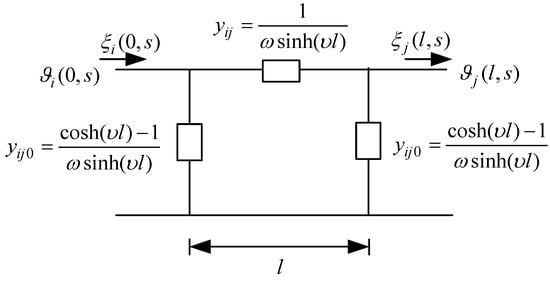
Figure 3.
π-Type equivalent circuit of the IES.
Therefore, the unified generalized admittance matrix Y of the IES is expressed as Equation (19):
where is the Laplace form of the admittance matrix and is the generalized equivalent ground admittance of bus i.
3. IES Time-Domain Two-Port Model Considering Delay
We rewrite Equations (13) and (14) into a unified format:
where is the state quantity, and and are constant coefficient matrices whose values are and , respectively. Considering that the IES is a complex space–time system, it is assumed that the discrete space–time interval of interest is , and the space and time step is and , respectively. Using the difference scheme constructed in [15] for modeling, the constant coefficient matrices are set as the transfer matrix from to , the transfer matrix from to , and the transfer matrix from to . According to the superposition theorem, the recurrence relation of the IES differential grid can be expressed by Equation (21):
where represents the value of the state quantity at time t at x. According to [25], let be the identity matrix, and the analytical formula of can be expressed by Equations (22)–(24).
Extending to (), represents the set of state quantities at all positions at time t; then, when , through the idea of superposition, Equation (21) can be rewritten as Equation (25):
where is a lower triangular matrix, so complex matrix exponentiation operations can be avoided in the calculation. By further generalizing the time to (), we can rewrite Equation (25) as Equation (26):
where Equation (26) represents the transfer of the state quantity to the state at the moment in the unified network.
Assuming that the state quantities of the starting point of the branch under study are and , the state quantities of the endpoint are and , the space–time step size between two buses is 3 (i.e., ), and is the transfer matrix of the starting state quantity to the end state quantity, which is a part of ; then, Equation (26) can be expanded as Equation (27).
Equation (27) is transformed into Equation (28) after separating the IQ and EQUATION.
Through the Laplace domain generalized admittance matrix established above, without considering the time delay, the state quantity relationship of the four systems at time t can be expressed by Equation (29):
where , , and N are the number of IES system buses. However, after adding the time delay, the influence of the transfer of the spatiotemporal state on the generalized admittance matrix should be considered. Assuming that the distances between adjacent buses of the studied system are all equal to , the medium transmission time of adjacent buses is , and [t − k,t] is the time window. Then, for the heat, natural gas, and MHES networks, the real-time state quantity relationship at time t can be rewritten as Equation (30).
In particular, as is a lower triangular matrix, timing state quantities can be directly obtained by matrix multiplication. Therefore, the IES time-domain two-port model considering time delay avoids multiple recursive iterations caused by the time delay in the calculation. This model also eliminates the complex calculation process at the intermediate segment point and significantly improves the operation efficiency.
4. IDR Modeling
Demand side management (DSM) is a priority way to improve energy efficiency [26], and is one of the most commonly used management methods of electricity consumption management. DSM can reduce the peak power demand (kW) and electricity consumption (kWh) of electricity [27]. The most commonly used DSM methods include peak load reduction, load shifting, increasing load flexibility, and reducing energy consumption [28]. For IDR, additional consideration should be given to modeling replaced loads [29]. Let i be the index of a bus; referring to the classification of traditional power DR, IES user-side DR loads (electrical, thermal, and natural gas loads) can be classified into fixed , adjusted , shifted , and replaced loads according to the interactive response characteristics. The MHES is divided into two parts: nonmobile energy storage (the discharge power at bus i is ) and electric vehicle hydrogen energy storage participating in mobile dispatch (the discharge power at bus i is ). To adapt to the model in this study, this study enables the nonmobile energy storage to meet the dispatching demand of the shifted load (to simplify the study, let ). Moreover, the electric vehicle hydrogen energy storage, together with the heat, natural gas, and power networks, can meet the adjusted load and replaced load scheduling requirements. Let be the power load after DR, be the power load before DR, and be the response power value. The demand side model of IDR is established as Equation (31).
In general, IDR scheduling can be achieved in direct or indirect ways as follows: (1) In the direct load reduction, managers stimulate consumers to reduce part of the load by providing incentives, which corresponds to . (2) In the multienergy demand coupling on the user side, some users will use electricity to meet their thermal demand. Hence, IDR can encourage the increase in thermal demand to reduce the power load, which corresponds to . According to the above analysis, Equation (31) is supplemented with Equation (32).
is the amount of total load reduction, is the amount of electrical load reduction, is the amount of electrical load reduction because of the increase in heat supply on the supply side, is the amount of electrical load reduced because of the increase in the supply of natural gas on the supply side, and is the amount of electrical load reduction because of the increase in the supply side of the MHES output.
4.1. Modeling of Multienergy Coupling Equipment
The energy coupling devices in this study are microturbine (MT), electric air conditioner (AC), gas boiler (GB), and power converter (PC).
- (a)
- Power grid to gas network: MT
The relationship between generator output and natural gas consumption can be expressed by Equation (33):
where represents the gas consumption rate (m3/s) of MT, represents the slope of the fuel curve (m3/(kW·s)), and represents the electrical power output of MT.
- (b)
- Power grid to thermal network: MT and AC
MT emits high-temperature flue gas as a by-product when generating electricity, and the heat in the flue gas can supply heat to the thermal network. In general, the MT power generation determines the thermal output, so the heat production of MT can be expressed by Equation (34) [7]:
where is the gas heat recovery rate, is the thermal output of MT (kW), and LHV is the lower heating value of gas (MJ/ m3).
AC is a device that converts electricity into heat, and the energy coupling relationship is expressed by Equation (35):
where is the heat generated by the AC, is the heating efficiency of the AC, and is the electrical power required by the AC.
- (c)
- Gas network to thermal network: GB
The relationship between output power and gas consumption of GB is shown in Equation (36):
where is the GB’s efficiency, is the GB’s thermal power output (kW), and is the GB’s gas consumption rate (m3/h).
- (d)
- MHES network to power grid: PC
As part of the user’s electrical load demand can be replaced by heat, natural gas, and MHES on the supply side, according to the above modeling, Equation (32) can be rewritten as Equation (33):
where is the electric load reduction value, is the natural gas flow, is the increased heat output of the MT, is the reduced heating power of the electric air conditioner, is the increased natural gas input for the MT, is the increased output of the MHES, and , , and are the coupling coefficients.
4.2. Objective Function of IDR
Because PBDR encourages load shifting rather than load shedding, it provides the ability to strategically increase and decrease demand [11]. Based on the model of PBDR for electricity, the relationship between electricity demand and electricity prices is generally inversely proportional. In order to meet the need of “shaving peaks and filling valleys” for IDR, a segmented curve for time-shifted electricity prices should be designed. The curve is expressed as Equation (39):
where is the time-shifted electricity price of IES users, is the normal electricity price when no DR is performed, is the electricity price correction coefficient during the peak period of electricity consumption, is the electricity price correction coefficient during the valley period of electricity consumption, is the peak period of electricity consumption, and is the valley period of electricity consumption.
Since the MHES is connected to the power grid bus through the PC, and the MHES is mostly on the user side, during the peak period of electricity consumption, the discharge demand of the MHES increases due to the increase in electricity prices; during the valley period of electricity consumption, due to the lower electricity price, the MHES will be in the charging state. Therefore, for users, the cost of using MHES will generally be lower than the direct power purchase average cost under PBDR. Therefore, in theory, if the MHES is scheduled at the right time, the MHES can participate in the IDR’s “peak shaving and valley filling”. In addition, since the MHES’s scheduling process can reduce the use of fossil fuel vehicles, the MHES will reduce the original environmental cost when participating in IDR.
Based on the above analysis, the optimal IDR objective of a grid-connected IES is to minimize the total annual planning cost Ftotal, including IDR grid operation cost f1, natural gas purchase cost f2, environmental cost f3, and MHES dispatch cost f4. The expression is as shown in Equation (40).
The expression of grid operating cost f1 is shown in Equation (41):
where T is the time series; is the price of electricity purchased at time t; is the price of electricity sold at time t; is the electricity purchased at time t; is the electricity sold at time t; and are the charging and discharging power of fixed energy storage, respectively; and are the binary variables that respectively control the charging and discharging of MHES (a value of 1 means charging/discharging, and 0 means that the energy storage has no action); is the cost of MHES charging and discharging loss; and K1 is the total number of fixed energy storage.
The natural gas purchase cost f2 is expressed by Equation (42):
where and are the gas purchase cost of MT and GB, respectively, and is the price of gas.
The environmental cost f3 is expressed by Equation (43):
where K1 is the total number of coupled devices using natural gas, k is the index of coupled devices, is the unit cost of pollutants for device k, and and are the unit pollutant emissions of MT and GB, respectively. is the unit cost of pollutants for gasoline used by a fuel vehicle, and are the unit pollutant emissions of gasoline.
The dispatch cost of MHES f4 is expressed by Equation (44):
where is the maintenance cost of MHES, and is the electricity provided by MHES for the power network.
4.3. IDR Constraints
4.3.1. Energy Balance Constraints
The IES operation should satisfy the electrical balance and thermal balance, as shown in the following two equations:
where is the total generation power of the distributed generation (DG) in the grid, is the total electrical load in the grid, and is the total load in the heat grid.
4.3.2. Equipment Output Constraints and Energy Storage Constraints
Equipment output constraints and energy storage constraints
where , , , and represent the maximum output value of the corresponding equipment at time t in bus i, and and represent the maximum charging and discharging power of conventional energy storage and fixed hydrogen energy storage at bus i at time t, respectively. Meanwhile, the last two constraints linearize the two 0–1 variables.
4.3.3. Energy Purchase Constraints
Energy purchase constraints
where and are the maximum natural gas flow purchased by the MT and GB at time t by bus i, and is the maximum power capacity purchased by the IES from the bulk system.
4.3.4. Demand Response Constraint
This constraint is used to prevent great impact on the user’s basic energy demand from IDR.
4.4. IDR Model Considering the Delay
When designing the IDR process, since the time scale of intraday optimization is often smaller than the energy transmission delay, day-ahead optimization should be performed before intraday optimization. The purpose of day-ahead optimization is to obtain the optimal load configuration without considering the time delay, and the purpose of intraday optimization is to obtain the load configuration result considering the time delay based on the day-ahead optimization. Both day-ahead optimization and intraday optimization follow the above objective function and constraints; the only difference is that intra-day optimization requires delay correction. Therefore, this section will propose a delay correction method for intraday optimization.
Let the differential spatiotemporal steps of the thermal network branch be and , the differential spatiotemporal steps of the natural gas network be and , and the differential spatiotemporal steps of the MHES network be and . We assume that the length of the branch between all adjacent buses in the thermal network is , and the heat flow direction is from other buses to bus i. It can be derived from Equation (30) that the state quantity of bus i at time t can be described by the state quantities of other buses in the system:
where is obtained from through elementary row transformation. The transformation method is to exchange the corresponding row in after matching the bus index in according to the distance. The content of the corresponding row in of buses with the same distance from bus i is the same. is an integer multiple of . In the same way, the expressions of the natural gas network and MHES network can be obtained.
Based on the above modeling, we can obtain the bus energy power expressions of four networks. Let and be the injection EQ of bus i and the set of all the IQ of all buses, respectively; is the number of buses in a system, and is the energy power in bus i of a system. As the IQ of buses in actual production is relatively easy to obtain, this study will use the IQ of buses to derive the power expression and the power of the power system to represent the power of the natural gas network and the MHES network. Let represent the i-th row of ; then the power expression can be expressed by Equation (51).
We consider a special branch (Figure 4) that initially has no power flow, and the time for power to flow from one bus to the next is . The influence of the power source on bus 1 (or a bus directly controlled by IDR) on the load on bus 4 (end of the branch) will be investigated below, . Suppose that a scheduling command is issued at time t, and the power source immediately issues one unit of power (or one power unit) whose length is one unit length in the pipeline. Moreover, suppose that is the set of each bus’s IQ at time t, and is the EQ of bus 4. In this case, Equation (48) can be rewritten as Equation (52):
when , we can obtain Equation (53).
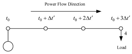
Figure 4.
Special branch in the IES.
From Equation (53), when studying the scheduling feature, the power changes on all buses are only affected by the source, and the delay is proportional to the distance from the bus to the source. Through the above analysis, considering that the correct scheduling should be based on the correct state quantity, ideally, the state quantity at a bus will become a fixed value in a short time after the change. Therefore, a system with a time delay can be regarded as a transient system (e.g., a power system) that sequentially and slowly updates the state quantity of each bus along the branches over time. Therefore, for the IES in this study, Equation (51) can be introduced into the more mature day-ahead planning method, and the planning solution considering the time delay can be obtained.
According to this idea, the designed process of IDR is as follows. The detailed flow chart is shown in Figure A1 in Appendix A.
(a) Before performing day-ahead planning, use the breadth-first algorithm, starting from each bus of the IES system, to find the shortest path to all other buses, and record it in matrix . The row label of is the number of the search starting bus (in order from 1), the column label is the number of all other buses, and the matrix elements are the shortest path between two buses. (For example, represents the shortest time taken for power flow to flow from bus a to bus b.)
(b) Input day-ahead forecast data on the supply and load sides.
(c) Use a commercial solver (Matlab Gurobi) to solve the control plan of the day before the IES (including work plans of coupling equipment, the thermal power plant, etc.) using the objective function (Equation (40)) and the constraints (Equations (45)–(49)).
(d) Read the element value related to the control plan in and correct the instruction time.
(e) The next day, update the intraday forecast data on the supply side and the load side of a specific scenario.
(f) Using the objective function (Equation (40)), the constrains (Equations (33)–(39), (41)–(49)) and delay correction equations (Equation (51), based on the day-ahead control plan, use a commercial solver (Gurobi) to solve the intraday IES control plan (e.g., DG output, energy storage state control, and load reduction plan).
(g) Output the optimal IDR scheduling plan of the IES and execute it.
5. Case Study
To verify the validity of the time-domain two-port model considering the delay, a simulation analysis is carried out in an IES. The IES is composed of a 51-bus thermal network [30], a 34-bus natural gas network [31], and an IEEE 14 bus standard system [32]. To simplify the calculation, a reasonable assumption is made here; that is, the topology of the MHES traffic network is consistent with the IEEE 14 bus network. There are also hydrogen electrolysis stations of the MHES network at the power generation buses of the power system. The load bus of the power system is also the hydrogen load bus of the MHES network.
Figure 5 shows the system structure of the example, where “e” represents the power network, “g” represents the natural gas network, and “h” represents the thermal network. The black numbers in Figure 5 represent the bus index of each network, and the green numbers represent the position of the power system buses corresponding to nonpower system buses.
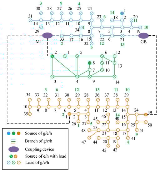
Figure 5.
IES structure in this case.
As the research object is the DR to the electrical load, the thermal load and the gas load are always satisfied by default. According to the operating characteristics of the IES, the following conditions are given for simulation:
(1) The voltage and current of power sources; (2) the initial temperature distribution of the heat branch and the temperature of the heat source; and (3) the initial pressure and flow distribution of the natural gas branch, the pressure distribution of the natural gas source, and the flow distribution of the gas load bus. The simulation step size of the power system branch is 1 min, and the differential space–time step size of the thermal branch is 72 and 3 min; the differential space–time step size of the natural gas branch is 4500 and 5 min.
5.1. Time-Domain Two-Port Model Validation: Part 1
In this case, we assumed that each bus has flexible loads and flexible energy storage. Using this assumption, the power generation transfer distribution factor (GSDF) characteristics of the power system can be compared to verify the correctness of the time-domain two-port model in this study.
Taking buses 29 and 30 of the thermal system as an example, the space–time distances of the two buses are and , namely, 9 and 540 m. Let the flow rate be , , and , and we obtain and . Considering that the relationship between temperature and heat can be assumed to be linear, the steady-state value can be ignored to analyze the effect of power variation alone. If the heat load of bus 29 is reduced by 1 MW at this time, it can be known from Equation (4) that and . By substituting the values into Equations (27), (28), and (48), we can obtain and . This result means that after , the temperature of bus 30 increases by , and the thermal power increases by 5.6 kW. Taking buses 29 and 34 of the thermal system as other examples, the space–time distance between the two buses is and , when the heat load of bus 29 is reduced by 1 MW, , ; that is, the temperature of bus 34 increases by , and the thermal power increases by 2.7 kW. The result is consistent with the law of the GSDF in the power system, which can reflect the effectiveness of the model proposed in this study.
5.2. Time-Domain Two-Port Model Validation: Part 2
To verify the feasibility of the model proposed in this study in DR, in this case, we consider the synchronization effect of a source bus power change on a distant bus within one day. Taking buses 33, 34, 32, and 25 of the natural gas system as an example, there is a coupling device, MT, on bus 33, and the space–time distances among buses 34, 32, 25, and 33 in the natural gas system are 3, 4, and 7 times of and , respectively. We assume that the system pressure in a steady state is 4000 kPa, and the average flow rate is , and the MT on bus 33 increases the electricity output by 1000 kW. The relationship between pressure and flow rate can be assumed to be linear, so similar to the thermal system, the steady-state values can be ignored to analyze the effects of power changes alone. Thus, the changes in air pressure and flow corresponding to bus 33 are (kPa) and (m3/s), respectively.
Figure 6 depicts the pressure and flow curves of several buses, assuming that the MT on bus 33 increases the electricity output by 1000 kW at t = 0. From Figure 6, the pressure and flow of bus 34 fluctuate first, having the largest fluctuation. Then, the pressure and flow of buses 32 and 25 fluctuate, and the fluctuation gradually becomes smaller. This result reflects the influence of time delay on different buses in the natural gas system, which can prove the validity of the two-port model proposed in this study, thereby providing a theoretical reference for IDR considering time delay.
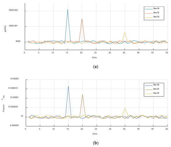
Figure 6.
Pressure and flow curves of several buses: (a) curves of pressure fluctuation of buses; (b) curves of flow fluctuation of buses.
5.3. IDR Validation
The day-ahead load forecast is set based on the energy consumption data recorded from institutional buildings in Singapore from [33] and as shown in Figure A2 in Appendix B. The values of coefficients in the case study are shown in Table A1. The device parameters in the case are from [7].
Figure 7 compares the running costs with and without the IDR method. During the peak electricity consumption period between 8:00 and 22:00, the operating cost with IDR is significantly lower than that without IDR, and the total daily operating cost is USD 6234 and USD 6324, respectively, which shows that the model proposed in this study can reduce the operating cost of the IES and then can reduce the management difficulty when the load fluctuates greatly.
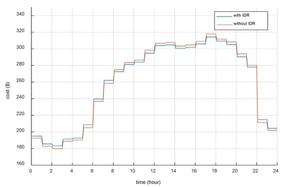
Figure 7.
Running costs with and without the IDR.
Figure 8 depicts a further simulation of the scheduling process on this day, which shows the optimal scheduling results of multiple energy equipment and loads. The upper part of the horizontal axis is the energy output, and the lower part of the horizontal axis is the energy input. “MH discharge” is the discharge power of MH, “MH charge” is the charging power of MH, “AC input” is the power consumption of the air conditioner, “Load” is the power load, “DG” is the power generated by DG, “Buy” is the power purchased, and “MT” is the electricity output of the MT.
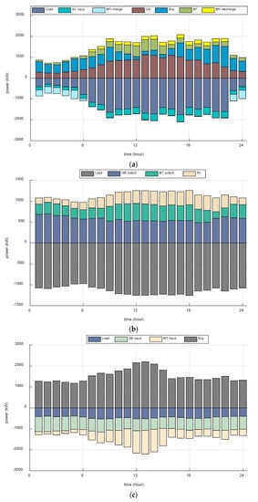
Figure 8.
Optimal scheduling results of energy equipment and loads: (a) optimal scheduling results in electrical network; (b) optimal scheduling results in thermal network; (c) optimal scheduling results in gas network.
As can be seen from Figure 8a, from 20:00 to 6:00 of the next day, electricity demand is mainly met by purchased electricity because of the low electricity price. At this time, MH is mainly in the charging state, and the output of the DG (which contains PV) is also low. During the period of 6:00–19:00, the purchased electricity is reduced because of the higher electricity price, and the MT and the DG jointly meet most of the electricity demand. Notably, MH also discharges at this time to support the operation of auxiliary services in the power market and the operation of MH-based electric equipment, further reduce the operating cost of IES, and help to promote energy supply and demand balance. Figure 8b shows that in this IES system, the heat output of the GB is relatively stable throughout the day, and the GB output decreases slightly when the electricity consumption peaks. The heating of the air conditioner is satisfactory. From Figure 8c, we can see that as the MT output increases, the purchase volume of the natural gas network also increases. The correctness of the model and method proposed in this study is verified.
6. Discussion
The feasibility of the method proposed in this study depends more on the intelligence and autonomy of the edge devices of the energy network, and almost all similar studies are also based on this premise. At present, the emergence of some hydrogen energy pilots and equipment (such as “Sesame Solar”) provides a solid foundation for future clean energy utilization, but there is currently no suitable dispatch mechanism to match it. Furthermore, each new energy device or energy type that emerges has a hugely transformative impact on existing research or existing facilities. Therefore, after the preliminary research in this study, more follow-up research should further explore a new scheduling mechanism for the impact.
7. Conclusions
Given that hydrogen energy utilization has almost no carbon dioxide emissions and can replace high-carbon fuels in many industries, such as transportation, power supply, and industrial production, this study establishes a universal regional-level IES architecture on the distribution grid side that integrates MHES. Moreover, considering the time delay characteristics of the nontransient system, a two-port model integrating electricity, heat, natural gas, and hydrogen is established. In the application of DR, the rationality and effectiveness of the IES model proposed in this study are verified. In the current mainstream hydrogen production methods, owing to the differences in the resource endowment in the region, the cost of hydrogen production is different, which makes achieving optimal regional resource allocation efficiency difficult. Therefore, the MHES proposed in this study has good market prospects. In addition, the accurate time delay management of the IES system is conducive to implementing “peak shaving and valley filling,” further reducing the operating cost of the IES system, and promoting the construction of the global energy Internet. Since the current research on MHES is somewhat preliminary, the future efforts of this research will focus on refining the various application scenarios of MHES, and will dig out more modeling ideas for hydrogen energy utilization.
Author Contributions
Conceptualization, H.C.; simulation, H.C.; writing H.C.; editing, H.C.; methodology, Q.A. All authors have read and agreed to the published version of the manuscript.
Funding
This research was funded in part by the National Natural Science Foundation of China (U1866206) and in part by the National Key R&D Program of China (2021YFB2401203).
Conflicts of Interest
The authors declare no conflict of interest.
Appendix A

Figure A1.
The designed process of IDR.
Appendix B

Figure A2.
Day-ahead load forecast.
Table A1.
Values of coefficients in the case study.
Table A1.
Values of coefficients in the case study.
| Coefficient | Values | Coefficient | Values | |
|---|---|---|---|---|
| 10 | 22:00–7:59 | 0.06 | ||
| 8:00–21:59 | 0.11 | |||
| 0.9 | 22:00–7:59 | 0.05 | ||
| 8:00–21:59 | 0.22 | |||
| 2 | 0.005 | |||
| 0.8 | 0.045 | |||
| 0.9 | 0.012 | |||
| 0.9 | 0.012 | |||
References
- Wang, Y.; Zhang, N.; Kang, C.Q. Review and prospect of optimal planning and operation of energy hub in Energy Internet. Proc. CSEE 2015, 35, 5669–5681. [Google Scholar]
- Geidl, M.; Koeppel, G.; Favre-Perrod, P.; Klockl, B.; Andersson, G.; Frohlich, K. Energy hubs for the future. IEEE Power Energy Mag. 2007, 5, 24–30. [Google Scholar] [CrossRef]
- Xie, S.; Hu, Z.; Wang, J.; Chen, Y. The optimal planning of smart multi-energy systems incorporating transportation, natural gas and active distribution networks. Appl. Energy 2020, 269, 115006. [Google Scholar] [CrossRef]
- Ma, Y.; Wang, H.; Hong, F.; Yang, J.; Chen, Z.; Cui, H.; Feng, J. Modeling and optimization of combined heat and power with power-to-gas and carbon capture system in integrated energy system. Energy 2021, 236, 121392. [Google Scholar] [CrossRef]
- Liu, X.; Wu, J.; Jenkins, N.; Bagdanavicius, A. Combined analysis of electricity and heat networks. Appl. Energy 2016, 162, 1238–1250. [Google Scholar] [CrossRef]
- Wang, C.; Lv, C.; Li, P.; Song, G.; Li, S.; Xu, X.; Wu, J. Modeling and optimal operation of community integrated energy systems: A case study from China. Appl. Energy 2018, 230, 1242–1254. [Google Scholar] [CrossRef]
- Panah, P.G.; Cui, X.; Bornapour, M.; Hooshmand, R.-A.; Guerrero, J.M. Marketability analysis of green hydrogen production in Denmark: Scale-up effects on grid-connected electrolysis. Int. J. Hydrog. Energy 2022, 47, 12443–12455. [Google Scholar] [CrossRef]
- Han, G.; Kwon, Y.K.; Kim, J.B.; Lee, S.; Bae, J.; Cho, E.; Lee, B.J.; Cho, S.; Park, J. Development of a high-energy-density portable/mobile hydrogen energy storage system incorporating an electrolyzer, a metal hydride and a fuel cell. Appl. Energy 2020, 259, 114175. [Google Scholar] [CrossRef]
- Li, P.; Wang, Z.; Wang, N.; Yang, W.; Li, M.; Zhou, X.; Yin, Y.; Wang, J.; Guo, T. Stochastic robust optimal operation of community integrated energy system based on integrated demand response. Int. J. Electr. Power Energy Syst. 2021, 128, 106735. [Google Scholar] [CrossRef]
- Xiang, Y.; Cai, H.; Gu, C.; Shen, X. Cost-benefit analysis of integrated energy system planning considering demand response. Energy 2020, 192, 116632. [Google Scholar] [CrossRef]
- Finn, P.; Fitzpatrick, C. Demand side management of industrial electricity consumption: Promoting the use of renewable energy through real-time pricing. Appl. Energy 2014, 113, 11–21. [Google Scholar] [CrossRef]
- Tan, H.; Yan, W.; Ren, Z.; Wang, Q.; Mohamed, M.A. A robust dispatch model for integrated electricity and heat networks considering price-based integrated demand response. Energy 2022, 239, 121875. [Google Scholar] [CrossRef]
- Zheng, S.; Sun, Y.; Li, B.; Qi, B.; Zhang, X.; Li, F. Incentive-based integrated demand response for multiple energy carriers under complex uncertainties and double coupling effects. Appl. Energy 2021, 283, 116254. [Google Scholar] [CrossRef]
- Bahrami, S.; Sheikhi, A. From demand response in smart grid toward integrated demand response in smart energy hub. IEEE Trans. Smart Grid 2015, 7, 650–658. [Google Scholar] [CrossRef]
- Huang, W.; Zhang, N.; Kang, C.; Li, M.; Huo, M. From demand response to integrated demand response: Review and prospect of research and application. Prot. Control. Mod. Power Syst. 2019, 4, 12. [Google Scholar] [CrossRef]
- He, L.; Lu, Z.; Geng, L.; Zhang, J.; Li, X.; Guo, X. Environmental economic dispatch of integrated regional energy system considering integrated demand response. Int. J. Electr. Power Energy Syst. 2020, 116, 105525. [Google Scholar] [CrossRef]
- Li, X.; Tian, G.; Shi, Q.; Jiang, T.; Li, F.; Jia, H. Security region of natural gas network in electricity-gas integrated energy system. Int. J. Electr. Power Energy Syst. 2020, 117, 105601. [Google Scholar] [CrossRef]
- Ceseña EA, M.; Mancarella, P. Energy systems integration in smart districts: Robust optimization of multi-energy flows in integrated electricity, heat and gas networks. IEEE Trans. Smart Grid 2018, 10, 1122–1131. [Google Scholar] [CrossRef]
- Parra, D.; Valverde, L.; Pino, F.J.; Patel, M.K. A review on the role, cost and value of hydrogen energy systems for deep decarbonisation. Renew. Sustain. Energy Rev. 2019, 101, 279–294. [Google Scholar] [CrossRef]
- Yao, S.; Gu, W.; Lu, S.; Zhou, S.; Wu, Z.; Pan, G.; He, D. Dynamic optimal energy flow in the heat and electricity integrated energy system. IEEE Trans. Sustain. Energy 2021, 12, 179–190. [Google Scholar] [CrossRef]
- Chen, Q.; Hao, J.H.; Chen, L. Integral transport model for energy of electric-thermal integrated energy system. Autom. Electr. Power Syst. 2017, 41, 7–13. [Google Scholar]
- Yang, J.W.; Zhang, N.; Kang, C.Q. Analysis Theory of Generalized Electric Circuit for Multi-energy Networks—Part One Branch Model. Autom. Electr. Power Syst. 2020, 44, 21–32. [Google Scholar]
- Guo, P.; Han, G.; Hua, B. The energy postulate and choice of independence state parameters of the thermodynamic system. Coll. Phys. 2004, 23, 27–29. [Google Scholar]
- Gu, W.; Lu, S.; Yao, S.; Zhuang, W.; Pan, G. Hybrid time-scale operation optimization of integrated energy system. Electr. Power Autom. Equip. 2019, 39, 203–213. [Google Scholar]
- Alipour, M.; Zare, K.; Zareipour, H.; Seyedi, H. Hedging strategies for heat and electricity consumers in the presence of real-time DR programs. IEEE Trans. Sustain. Energy 2019, 10, 1262–1270. [Google Scholar] [CrossRef]
- Jabir, H.J.; Teh, J.; Ishak, D.; Abunima, H. Impacts of demand-side management on electrical power systems: A review. Energy 2018, 11, 1050. [Google Scholar] [CrossRef]
- Tronchin, L.; Manfren, M.; Nastasi, B. Energy efficiency, demand side management and energy storage technologies—A critical analysis of possible paths of integration in the built environment. Renew. Sustain. Energy Rev. 2018, 95, 341–353. [Google Scholar] [CrossRef]
- Jing, R.; Xie, M.N.; Wang, F.X.; Chen, L.X. Fair P2P energy trading between residential and commercial multi-energy systems enabling integrated demand-side management. Appl. Energy 2020, 262, 114551. [Google Scholar] [CrossRef]
- Duhr, P.; Christodoulou, G.; Balerna, C.; Salazar, M.; Cerofolini, A.; Onder, C.H. Time-optimal gearshift and energy management strategies for a hybrid electric race car. Appl. Energy 2021, 282, 115980. [Google Scholar] [CrossRef]
- Lu, S.; Gu, W.; Meng, K.; Yao, S.; Liu, B.; Dong, Z.Y. Thermal inertial aggregation model for integrated energy systems. IEEE Trans. Power Syst. 2020, 35, 2374–2387. [Google Scholar] [CrossRef]
- Gaslib. GasLib-135[EB/OL]. Available online: http://gaslib.zib.de/ (accessed on 3 August 2021).
- Matpower. IEEE-14[EB/OL]. Available online: https://matpower.org/ (accessed on 3 August 2021).
- Yang, J.; Ning, C.; Deb, C.; Zhang, F.; Cheong, D.; Lee, S.E.; Sekhar, C.; Tham, K.W. k-Shape clustering algorithm for building energy usage patterns analysis and forecasting model accuracy improvement. Energy Build. 2017, 146, 27–37. [Google Scholar] [CrossRef]
Publisher’s Note: MDPI stays neutral with regard to jurisdictional claims in published maps and institutional affiliations. |
© 2022 by the authors. Licensee MDPI, Basel, Switzerland. This article is an open access article distributed under the terms and conditions of the Creative Commons Attribution (CC BY) license (https://creativecommons.org/licenses/by/4.0/).