Eigenstructure through Matrix Adjugates and Admissible Pairs

Abstract

The traditional eigenstructure assignment method is reconsidered in this paper, shedding light on its nature and some of its properties. The approach is through matrix adjugates which enable a more eloquent decomposition compared to the lumped solution usually obtained through matrix null spaces. Based on the new approach, the admissible pair $(w,z)$ is formalized. The new approach enables an alternative methodology to the determination of the permissible closed loop eigenvector subspaces and the might be termed the companion input-subspace. Such approach renders the method a formulae-based method as $w$ and $z$ are now obtained formula-wise as opposed to being extracted out of a lumped solution. Compared to the traditional method, the study reveals information such as $w$ and $z$ are independently and explicitly determined. Moreover, newly assigned eigenvalues always result in $z\ne 0$, the input matrix $B$ does not influence $z$ and a fundamental feature of the open loop characteristic polynomial is exposed. Furthermore, closed loop eigenvectors associated with repeated eigenvalues can be explicitly computed by means of differentiation as opposed to null space determination. A special form of system representation is highlighted, which considerably eases the calculations. The myriad concepts pointed out have been demonstrated and authenticated through carefully selected examples involving real, complex, repeated eigenvalues, and two practical systems of an electrical nature.

1. Introduction

Eigenvalue assignment on its own is the first approach one looks for when it comes to stabilization and control of a system’s growth or decay. To address issues such as shape of response, maintaining system robustness, and insensitivity, a need arises to involve the eigenvectors as well as the eigenvalues in system design.

The first introduction of eigenvalue-eigenvector assignment in shaping system response was given in [1,2]. We are focusing on a particular approach namely the eigenstructure assignment, known earlier as the entire-eigenstructure assignment. We refer the reader to some books on the subject matter [3,4], to a survey [5], in addition to [6].

Early works on eigenstructure assignment were conducted by [1,2]. They identified the freedom offered by state feedback in specifying the closed loop eigenvectors as well as the closed loop eigenvalues. In addition, they provided a characterization of all attainable eigenvectors associated with a given set of eigenvalues. Other early researchers were [7,8,9,10] who provided algorithms for obtaining such attainable sets of eigenvectors. Though state and output feedback eigenstructure assignment cannot change uncontrollable eigenvalues, their associated eigenvectors may be chosen to a certain extent to improve the insensitivity and the robustness of the closed-loop system [11]. In a study by [12], the theory of eigenstructure has been applied to more precisely shape the modes involved in a vibrating system. An extensive flight control example is treated in [6]. A mention must be made of a book [13] regarding the application of eigenstructure method to avionics. There, the author has shown that no more than $m$ entries of any eigenvector can be chosen arbitrarily. A PhD thesis by [14] investigated the application of eigenstructure assignment to aircraft problems. Furthermore, textbooks’ treatment of eigenstructure is well-explained in [15,16].

Recent applications to a three-axis dynamic flight motion simulator has been conducted in [17]. The authors employed derivative PD state feedback together with a partial subset of the system eigenstructure. Both resulted in a simplified, more economical, and robust approach compared to the traditional eigenstructure approach. The case of large scale systems has been tackled by [18]. Partial eigenstructure assignment was used to derive a new parametric solution. The solution method involved inverses of lower order matrices, resulting in computational load reduction. In [19], the authors addressed a problem with output feedback, where only partial assignment is possible and a trade-off between sensitivity and stability should be exercised. Eigenstructure assignment methods for vibration cancellation and suppression in large space structures have been reviewed in [20]. In particular, a method known as orthogonal eigenstructure has been found to offer significant simplification of the design task. It also facilitates some experience-based design. An approach based on multibody aircraft dynamics rather than the conventional rigid-body configuration has been studied in [21]. The eigenstructure assignment proves a convenient approach since the differences between both types of aircraft are reflected in the eigenvalues and eigenvectors. Consequently, an implementation of a straightforward inner-loop control law accomplished desired aircraft requirements on damping and stiffness.

The eigenstructure method is now a well-established method for eigenvalue-eigenvector assignment using state and output feedback [6]. It is characterized by a determination of an eligible $n\times 1$ closed loop eigenvector $w$ together with an $m\times 1$ companion input-vector $z$. Both vectors result from a solution method based on the null space of a certain formulation of the feedback used. In its most simple form, the lumped solution is the null space solution of an augmented $n\times n+m$ matrix. Typically, the traditional eigenstructure method gives a lumped solution in the sense that both $w$ and $z$ are not independently obtained, but have be extracted out of a null space solution (an $n+m\times 1$ vector), where $w$ is extracted as the top $n$ entries and $z$ as the bottom $m$ entries.

As a numerical value, the null space solution overshadows (conceals) the nature and structure of both $w$ and $z$ even after decomposing the solution into its constituent parts. Any additional structural information is therefore welcomed as it provides further insight together with additional characterization. Both help in improving intuition, in easing calculations, and in reducing problem dimensionality throughout both analysis and design stages. This task is undertaken by our treatment utilizing the concept of matrix adjugates. We shall interchangeably refer to our method as either the adjugate method or the admissible pair method, while referring to the traditional method as the null space method.

What distinguishes our approach is the fact that the adjugate of a matrix is unique leading to a naturally scaled admissible pair [22,23,24,25]. This is not the case with the usual eigenstructure method as the null space may differ in the values of its entries depending on the method used to determine it. MATLAB provides two approaches to determine the null space which give different answers in terms of the resulting numbers, though both are eligible and lie within the same solution space. From that perspective, our method provides standardization through formula based determination of both $w$ and $z$. Such an approach reduces dimensionality and in the theoretical sense enables a form of parallelism.

The adjugate method deals with lower dimensional matrices. It involves matrix manipulation of order $n\times n$, in comparison to manipulation of $(2n+m)\times (n+m)$ matrices required by the null space method. The adjugate method accentuates the importance of the open loop characteristic polynomial overshadowed by many eigenvalue assignment methods. The role of $B$ is also demystified when adopting the admissible pair approach in the sense that it does not influence $z$. This is not apparent when using the null-space method.

The adjugate method is convenient whenever dealing with matrices of special forms such as the companion form adopted by MATLAB as its default method for control system representation. It turns out that such a form together with the adjugate method provides direct immediate information related to the open loop system such as: stability, the characteristic polynomial, left and right eigenvectors, the derivative of $z$ with respect to $\lambda$. Most important, this form provides direct formula-based determination of the closed loop eigenvectors enhancing the explicitness of the adjugate method when it comes to distinct and repeatedly assigned eigenvalues together with their associated eigenvectors.

We begin our study in Section 2 by briefing the eigenstructure involvement in shaping a system time response through left and right eigenvectors. We then outline two convenient approaches to the solution process through an admissible pair in Section 3. We pay a visit to the determination of left and right eigenvectors from the matrix adjugate point of view in Section 4. The core of our study is a formulation of the admissible pair through independent and explicit formula-based relations in Section 5; together with insightful relevant remarks. The tools are matrix adjugates and the open loop characteristic polynomial. Matrix adjugates efficiently lend themselves to a companion form adopted by MATLAB. Such a form simplifies many issues related to open loop and closed loop eigenvector determination; being formalized in Section 6. Extending the null space and a need for repetitive differentiation of the admissible pairs related to identical eigenvalues is proved in Section 7 and shown to be systematic and straightforward. In case of blending between the adjugate and the null space method regarding mixed calculations, a conversion between the two is essential as discussed in Section 8. Our investigation concludes with four examples; fully worked out to demonstrate and validate a number of conceptions introduced throughout the manuscript. The calculation and simulation tool is MATLAB.

Broadly, we summarize the contribution and novelty of our study as follows. The details are within the main body of the manuscript. All serve as advantageous features if compared to the traditional eigenstructure method.

• Contributing independent determination of the two main parameters $(w,\hspace{0.17em}z)$, together with explicit determination of $(w,\hspace{0.17em}z)$, rendering our method a formula-based method (Section 5).
• A decoupled computation of the pair $(w,\hspace{0.17em}z)$, thus enabling parallelism.
• Highlighting an important role played by the usually overlooked open loop characteristic polynomial when it comes to closed loop eigenvalue assignment.
• Presenting a particular matrix form which provides direct information regarding system structure, stability, and many other aspects of systems. Such form significantly eases the eigenvector assignment process (Section 6).
• Providing systematic determination of the closed loop generalized eigenvectors when dealing with repeated eigenvalue assignment (Section 7).
• Manipulating lower order matrices using the adjugate of a matrix.
• Presenting three fully worked out examples to demonstrate the convenience of the adjugate method. Theory related to a commonly encountered electronic circuit is also treated in Section 6. In addition, a practical application concerning a realistic system is presented in Example 4. It concerns a well-known industrial machine, namely the speed control of an armature control DC motor (Section 9).

2. The Eigenstructure Method in Brief

Since the location of eigenvalues alone do not specify a system response completely, a need arises to involve the associated eigenvectors. In doing so, one exercises additional control over the behavior of the system. An established fact concerning multi-input systems, i.e., $m>1$, is that the same set of eigenvalues can be specified through non-unique feedback matrices. Such non-unique $K$ matrices result in markedly unalike responses of a system. This is due to the differences in the eigenvectors assigned leading to systems of diversified structure and hence yielding different responses.

Regarding a simplified system response, things become clearer and informative when examining the forced time response $x(t)$ of a linear time-invariant system. It is given by [14].

$$x(t)={\displaystyle \sum _{i=1}^n{v}_i\hspace{0.17em}{e}^{{\lambda }_{i}t}\hspace{0.17em}{w}_i{}^{T}x(0)+}{\displaystyle \sum _{i=1}^n{v}_i\hspace{0.17em}{\displaystyle {\int }_0^t{e}^{{\lambda }_i(t-\tau )}\hspace{0.17em}{w}_i{}^{T}Bu(\tau )\hspace{0.17em}d\tau }}$$

(1)

where ${\lambda }_{\hspace{0.17em}\hspace{0.17em}i}$, $v_i$, and $w_i$ stand for a system eigenvalue together with its right and left associated eigenvectors. The role of (1) is discussed further in Example 1 and in full within Appendix A.

Scrutinizing (1), the eigenvalues determine the rate of decay or growth of the time response while the right eigenvectors $v_i$ prescribe the distribution of the modes. Regarding the left eigenvectors $w_i$ and since $w_i{}^{T}x(0)$ is a multiplying scalar, it clearly determines the amount each mode $v_i{e}^{{\lambda }_{j}t}$ participates to the response in both the transient (exemplified by $w_i{}^{T}x(0)$) and the steady state (exemplified by $w_i{}^{T}Bu(\tau )$).

Moreover, occasionally $w_i{}^{T}x(0)$ can be zero with some initial conditions, thus influencing the transient response. When the system is uncontrollable, the impact of the left eigenvectors is even more pronounced and more direct when compared with the impact of the right eigenvectors. This is because $w_i{}^{T}Bu(\tau )$ is zero irrespective of $u(\tau )$ when $w_i$ is a left eigenvector associated with an uncontrollable eigenvalue, thus, inhibiting the effect of $u(\tau )$.

Such recognition of the importance of left and right eigenvectors in shaping the dynamic response as exhibited by (1) and the freedom offered in their selection in the multi-input case have justified them a viable approach to systems in analysis and in design in both the transient and the steady state. Essentially, the purpose of eigenstructure control is the utilization of feedback to arrive at a suitable set of a system eigenvalues as well as their associated eigenvectors.

Such utilization is useful in optimizing the contribution of such system modes in the overall response, in organizing and coordinating mode distribution, and in specific cases, as a means of completely eliminating particular contributions if so desired.

3. Adoption of Two Convenient Forms to Determine the Admissible Pairs

The system and controller under considerations are given by

$$\stackrel{•}{x}=Ax+Bu\hspace{0.17em}\hspace{0.17em}\hspace{0.17em}\hspace{0.17em};\hspace{0.17em}\hspace{0.17em}\hspace{0.17em}x\in {ℝ}^n\hspace{0.17em}\hspace{0.17em},\hspace{0.17em}\hspace{0.17em}\hspace{0.17em}u\in {ℝ}^m\hspace{0.17em}\hspace{0.17em}\mathrm{where} \hspace{0.17em}\hspace{0.17em}1\le m\le n$$

(2)

$$u=K\hspace{0.17em}x$$

(3)

The closed loop system is therefore,

$$\stackrel{•}{x}=(A+BK)x$$

(4)

The eigenstructure assignment method involves a feedback matrix $K$ which assigns eigenvalues ${\lambda }_i$ using the pair $(w_i\hspace{0.17em},\hspace{0.17em}{z}_i)$, where $w_i$ is the associated $n\times 1$ closed loop eigenvector and $z_i$ is the associated companion $m\times 1$ input-vector.

As $w_i$ is a closed loop eigenvector pertinent to the eigenvalue ${\lambda }_i$, the following holds for any eigenvalue of algebraic multiplicity $1$.

$$(A+BK)w_i={\lambda }_{\hspace{0.17em}i}{w}_i$$

(5)

Two convenient rearrangements of (5) are to be used in our investigation. They are:

(i)

The null-space method [26] associated with the traditional eigenstructure method [7,8,16], where the system is expressed as.

$$[{\lambda }_i{I}_n-A\hspace{0.17em}⋮\hspace{0.17em}\hspace{0.17em}-B]\hspace{0.17em}\hspace{0.17em}\left[\begin{array}{c}{w}_i\\ K{w}_i\end{array}\right]=0\hspace{0.17em}\hspace{0.17em}\hspace{0.17em}\Rightarrow \hspace{0.17em}\hspace{0.17em}\hspace{0.17em}[{\lambda }_i{I}_n-A\hspace{0.17em}⋮\hspace{0.17em}\hspace{0.17em}-B]\hspace{0.17em}\hspace{0.17em}\left[\begin{array}{c}{w}_i\\ z_i\end{array}\right],\dots \mathrm{i}.\mathrm{e}.., z_i=K\hspace{0.17em}{w}_i$$

(6)

In which case [27,28,29,30]:

$$\left[\begin{array}{l}{w}_i\hfill \\ z_i\hfill \end{array}\right]=null(\left[\begin{array}{ll}{\lambda }_i{I}_n-A\hfill & ¦-B\hfill \end{array}\right])$$

(7)

(ii)

The adjugate method where the system is expressed as

$$({\lambda }_i{I}_n-A)\hspace{0.17em}{w}_i=B\hspace{0.17em}{z}_i$$

(8)

Using either rearrangement (7), or (8), the feedback matrix is calculated as below. Collectively, considering the $n$ assigned eigenvalues such that all $w_i$ are independent [6,9,15],

$$\left[\begin{array}{cccc}{z}_1& z_2& \cdots & z_n\end{array}\right]=K\left[\begin{array}{cccc}{w}_1& w_2& \cdots & w_n\end{array}\right]\Rightarrow \hspace{0.17em}\hspace{0.17em}\hspace{0.17em}K=\left[\begin{array}{cccc}{z}_1& z_2& \cdots & z_n\end{array}\right]{\left[\begin{array}{cccc}{w}_1& w_2& \cdots & w_n\end{array}\right]}^{\hspace{0.17em}-1}$$

(9)

A note on the use of $u=K\hspace{0.17em}x$ and not $u=-K\hspace{0.17em}x$ as in many books and research papers. The reason is that the former is the only representation which enables a reformulation as in (8). This is needed to end up with the input matrix $B$ not preceded by a negative sign, together with an open loop characteristic polynomial as $\left|{\lambda }_i{I}_n-A\right|$ which is always a monic polynomial irrespective of the system order $n$ being even or odd. This is a matter of convenience, minimizing negative signs throughout representations and human errors throughout manipulation.

The solutions of (7) are in general $\mu \hspace{0.17em}{w}_i$ and $\mu \hspace{0.17em}{z}_i$ where $\mu$ is a scalar multiplier. However, standardizing their values somehow is desirable, thus avoiding non-unique choices for eigenvector entries. This is helpful in our investigation; it is accomplished through the utilization of matrix adjugates which are unique. This renders our approach more appealing. Besides, matrix adjugates enable independent determination of the two solutions $w_i$ and $z_i$, in contrast to the null space method.

4. Right and Left Eigenvectors Revisited in the Light of Matrix Adjugates

The adjugate of a matrix is the transpose of its cofactor matrix [16,22,23,24,25]. Such name will be used instead of the adjoint which is widely used in many contemporary books on matrix theory and linear algebra. The old name “adjoint” nowadays refers to a matrix associated with the adjoint operator, where the adjoint is the conjugate transpose (not the transpose) of the cofactor matrix.

Matrix adjugates and eigenvectors are fundamental in our treatment of the subject matter. Mainly, we shall deal with the adjugate of ${\lambda }_i\hspace{0.17em}{I}_n-A$ and not of $A$ unless otherwise stated.

Definition 1.

The adjugate$adj(.)$of an$n\times n$matrix$M$is defined as

$$M\hspace{0.17em}adj(M)=adj(M)\hspace{0.17em}M=\left|M\right|I_n$$

(10)

It is unique and can be evaluated as the transpose of the matrix cofactors of$M$. Additional properties are scattered in almost any book on matrix theory [16,22,23,24,25].

Traditionally, following the definition of right ($w_i$) and left ($q_i$) eigenvectors of matrix $A$ as,

$$A\hspace{0.17em}{w}_i={\lambda }_i\hspace{0.17em}{w}_i \mathrm{and} q_i{}^{T}A={\lambda }_i\hspace{0.17em}{q}_i{}^T \mathrm{for} i=1,2,\cdots \dots ,n$$

(11)

or collectively as,

$$A\hspace{0.17em}\hspace{0.17em}W=W\hspace{0.17em}\Lambda ,\dots \mathrm{and} \dots Q^{\hspace{0.17em}T}A=\Lambda \hspace{0.17em}{Q}^T\dots$$

(12)

$W=\left[\begin{array}{ccc}{w}_1& \cdots & w_n\end{array}\right]$, $Q=\left[\begin{array}{ccc}{q}_1& \cdots & q_n\end{array}\right]$, and $\Lambda =diag({\lambda }_i)$.

Where post-multiplying the second relationship in (12) by $W$,

$$Q^{\hspace{0.17em}T}A\hspace{0.17em}W=\Lambda \hspace{0.17em}\hspace{0.17em}{Q}^{\hspace{0.17em}T}W\hspace{0.17em}\hspace{0.17em}\hspace{0.17em}\Rightarrow \hspace{0.17em}\hspace{0.17em}\hspace{0.17em}\hspace{0.17em}\hspace{0.17em}\hspace{0.17em}{Q}^{\hspace{0.17em}T}W\Lambda =\Lambda \hspace{0.17em}\hspace{0.17em}{Q}^{\hspace{0.17em}T}W$$

(13)

Equation (13) shows that $Q^{\hspace{0.17em}T}W$ and $\Lambda$ are commutative. Since matrices that commute with a diagonal matrix of distinct elements are themselves diagonal, we conclude that $Q^{\hspace{0.17em}T}W$ is diagonal, say $Q^{\hspace{0.17em}T}W=\sigma \hspace{0.17em}{I}_n$ [18]. A proper ordering of the $W$ and $Q$ columns ensures that. Furthermore, with proper scaling of $W$, one can make $Q^{T}W=I_n$. In which case, $Q^{\hspace{0.17em}T}=W^{-1}$. That is: the transpose of the left eigenvector matrix is the inverse of a properly scaled right eigenvector matrix. Conveniently, left eigenvectors are usually treated as row vectors $q_i{}^T$.

In light of the adjugate method, an alternative approach to the determination of left and right eigenvectors is the following.

Let $\lambda$ be an eigenvalue of $A$, then $A_{\lambda }=\lambda I_n-A$ is singular of zero determinant. Using (10),

$$A_{\hspace{0.17em}\lambda }\hspace{0.17em}adj(A_{\hspace{0.17em}\lambda })=adj(A_{\hspace{0.17em}\lambda })A_{\hspace{0.17em}\lambda }=\left|A_{\hspace{0.17em}\lambda }\right|\times I_n=0\times I_n=0_{n\times n}\hspace{0.17em}$$

(14)

When (10) is expressed as,

$$A_{\hspace{0.17em}\lambda }\hspace{0.17em}adj(A_{\hspace{0.17em}\lambda })=0_{n\times n}$$

A column of $adj(A_{\hspace{0.17em}\lambda })$ is a right eigenvectors of $A$.

When using the definition of a left eigenvector $q_i$ as in (11), i.e., $q_i{}^T({\lambda }_i\hspace{0.17em}{I}_n-A)\hspace{0.17em}=0$, and comparing it with (14) expressed as,

$$adj(A_{\hspace{0.17em}\lambda })A_{\hspace{0.17em}\lambda }=0_{n\times n}$$

A transposed left eigenvector ($q_i{}^T$) is a row of $adj(A_{\hspace{0.17em}\lambda })$.

N.B.: $q_i{}^T({\lambda }_i{I}_n-A)=0\Rightarrow ({\lambda }_i{I}_n-A^T)q_i=0$. Thus, a left eigenvector is a right eigenvector of $A^{\hspace{0.17em}T}$. It is a column of $adj({\lambda }_i{I}_n-A^T)\hspace{0.17em}$ which is a column of $\hspace{0.17em}{(adj({\lambda }_i{I}_n-A))}^T$ [23,24,25].

Whenever $A_{\hspace{0.17em}\lambda }=\lambda I_n-A$ is nonsingular as is the case when assigning an eigenvalue not that of $A$, the adjugate of $A_{\hspace{0.17em}\lambda }=\lambda I_n-A$ gives $m$ closed loop eigenvectors after post-multiplying $adj(A_{\hspace{0.17em}\lambda })$ by $B$, as will be proved below in Section 5.

5. Formula-Based Approach to the Determination of the Admissible Pair

The null space method [16,24,26] is a general purpose one; however, it is computationally the most demanding as it manipulates matrices of dimension $(2n+m)\times (n+m)$. Besides, it is not a direct method in the sense of not explicitly giving $w$ and $z$, neither a formula-based method.

Averting such shortcomings is therefore favorable. Our approach based on matrix adjugates fulfills such ambition as proved below.

Proposition 1. 

For${\lambda }_i$newly assigned (i.e., not already an eigenvalue of$A$),$z_i$is given by the open loop characteristic polynomial evaluated at the assigned eigenvalue${\lambda }_i$. Furthermore, the associated closed loop eigenvectors$w_i$are given by$w_i=adj({\lambda }_{\hspace{0.17em}\hspace{0.17em}i}{I}_n-A)B$

Proof. 

Using (6)

$$\left[\begin{array}{cc}{\lambda }_{\hspace{0.17em}i}{I}_n-A& -B\end{array}\right]\left[\begin{array}{c}{w}_i\\ z_i\end{array}\right]=0_{n\times m}$$

(15)

The solution ${\left[\begin{array}{cc}{w}_i& z_i\end{array}\right]}^{\hspace{0.17em}T}$ of (15) is, therefore, given by the null space of $\left[\begin{array}{cc}{\lambda }_{\hspace{0.17em}i}{I}_n-A& -B\end{array}\right]$. It remains the same solution as that of another matrix obtained by pre- multiplying (15) by any nonsingular matrix [24,27,28]. Since ${\lambda }_{\hspace{0.17em}i}{I}_n-A$ is nonsingular, its inverse is also nonsingular and therefore it qualifies as the pre-multiplying matrix, i.e., (15) has the same solution as the following system of equations [27,28].

$${({\lambda }_i{I}_n-A)}^{-1}\left[\begin{array}{cc}{\lambda }_i{I}_n-A& -B\end{array}\right]\left[\begin{array}{c}{w}_i\\ z_i\end{array}\right]=0_{n\times m}$$

(16)

which has the same solution as that of

$$\left[\begin{array}{cc}{I}_n& -\hspace{0.17em}{({\lambda }_i{I}_n-A)}^{-1}{B}_{n\times m}\end{array}\right]\left[\begin{array}{c}{w}_i\\ z_i\end{array}\right]=0_{n\times m}$$

(17)

$$\left[\begin{array}{cc}{I}_n& \frac{-\hspace{0.17em}adj({\lambda }_i{I}_n-A)B_{n\times m}}{\left|{\lambda }_i{I}_n-A\right|}\end{array}\right]\left[\begin{array}{c}{w}_i\\ z_i\end{array}\right]=0_{n\times m}$$

(18)

By direct substitution,

$$\left[\begin{array}{c}{w}_i\\ z_i\end{array}\right]=\hspace{0.17em}\hspace{0.17em}\mu \hspace{0.17em}\hspace{0.17em}\left[\begin{array}{c}adj({\lambda }_i{I}_n-A)B_{n\times m}\\ \left|{\lambda }_i{I}_n-A\right|I_{m\times m}\end{array}\right]\hspace{0.17em}\hspace{0.17em}\hspace{0.17em}\hspace{0.17em};\hspace{0.17em}\hspace{0.17em}\hspace{0.17em}\hspace{0.17em}\mu \ne 0\hspace{0.17em}\hspace{0.17em}\hspace{0.17em}\hspace{0.17em}\hspace{0.17em}$$

(19)

The most simple solution is when $\mu =1\hspace{0.17em}$, giving

$$w_i=adj({\lambda }_i{I}_n-A)B_{n\times m}$$

(20)

and

$$z_i\hspace{0.17em}=\hspace{0.17em}\left|{\lambda }_i{I}_n-A\right|I_m=({\lambda }_{\hspace{0.17em}i}{}^n+a_1{\lambda }_{\hspace{0.17em}i}{}^{n-1}+a_2{\lambda }_{\hspace{0.17em}i}{}^{n-2}+\cdots a_{n-1}{\lambda }_{\hspace{0.17em}i}+a_n)\hspace{0.17em}{I}_m$$

(21)

where $a_i\hspace{0.17em},\hspace{0.17em}\hspace{0.17em}i=1,\hspace{0.17em}\hspace{0.17em}2,\hspace{0.17em}\hspace{0.17em}\cdots ,\hspace{0.17em}\hspace{0.17em}n$, are the coefficients of the open loop characteristic polynomial.

Both $w_i\hspace{0.17em}\hspace{0.17em}\mathrm{and}\hspace{0.17em}\hspace{0.17em}{z}_i$ as in (20)–(21) are fundamental in our study and conveniently named an admissible pair.

Regarding the closed loop eigenvector $w_i$, it is most simple, formula-based, taken directly without any concern to elaborate scaling. Regarding intuition, $z_{\hspace{0.17em}i}$ is justifiably interpreted as the open loop characteristic polynomial evaluated at the eigenvalue ${\lambda }_{\hspace{0.17em}i}$ to be assigned. Besides, $z_i$ is also formula-based and is determined independently of $w_i$. Note that when $m>1$, $z_i$ is an $m\times 1$ column matrix.

Considerable use of (20) and (21) is expected in our treatment of the subject matter with regard to outlining system structure and easing numerical determinations. In addition, MATLAB is used to facilitate all the calculations needed through its readily available $null$ functions. We comment on the nature of the two $null$ functions, though we adhere to the use of one of them for comparison purposes. □

Remark 1.

(i)

An$n\times n$nonzero square matrix$M$can have any rank between$1$and$n$, but the rank of its adjugate is either$n$, or$1$.

Proof. 

 

If $M$ is nonsingular, its adjugate is nonsingular, thus of rank $n$.

If $M$ has rank $\le n-2$, the adjugate is identically a zero matrix as stated in [23,24].

We are left with $M$ of rank $n-1$, which is singular, having a nontrivial null space given by the adjugate. Invoking the following standard theory in linear algebra [23,24]:

$$\dim (null(M))=n-rank(M)$$

(22)

In our case, $rank(M)=n-1$, hence,

$$rank(adj(M))=\dim (null(M))=n-(n-1)=1$$

The importance of this remark is that the adjugate method can only give at most a single nonzero independent column when a matrix has rank $n-1$ as is the case in many assignment problems concerning eigenvalue reassignment or uncontrollable systems.

This implies that any reassigned eigenvalue using the adjugate method cannot give more than a single closed loop eigenvector even when $m>1$. □

(ii)

If${\lambda }_N$is not an eigenvalue of$A$i.e., newly assigned, then$z_i$and$w_i=adj({\lambda }_N\hspace{0.17em}{I}_n-A)B$cannot be zero and$w_i$has rank equal to$m$.

Proof. 

 

Since ${\lambda }_i$ is not an eigenvalue of A, ${\lambda }_N\hspace{0.17em}{I}_n-A$ is nonsingular, implying $\left|{\lambda }_N\hspace{0.17em}{I}_n-A\right|$ is non-zero. Since $z_{\hspace{0.17em}i}=\left|{\lambda }_{\hspace{0.17em}i}{I}_n-A\right|$ then $z_i$ is non-zero.

Furthermore, using properties of matrix adjugates, $adj({\lambda }_{\hspace{0.17em}i}{I}_n-A)$ is nonsingular having rank $n$. Hence,

$$rank(w_i)=rank(adj({\lambda }_i{I}_n-A)B)=\min (n,m)=m\ne 0$$

Therefore, the closed loop eigenvectors are nonzero and are $m$ in number. □

(iii)

Abiding by our selection of the admissible pair as in (20) and (21),$B$does not influence z_i.

Proof. 

 

Evident from $z_{\hspace{0.17em}i}=\left|{\lambda }_{\hspace{0.17em}\hspace{0.17em}i}{I}_n-A\right|$; obviously independent of $B$.

This fact could not have been thought of while adhering to the null space method. The reason is that the solution given by that method is a lumped solution containing both $w$ and $z$ where $B$ does not address either $w$ or $z$ as explicitly as the adjugate method. By a lumped solution, we mean an $n+m\times 1$ vector where $w$ is extracted as the top $n$ components and $z$ as the bottom $m$ components. □

(iv)

A Procedure for Shaping the Closed Loop Eigenvectors.

Having settled on desired ratios between no more than $m$ components of the closed loop eigenvectors [13], determine a $D_{m\times 1}$ matrix. To do that, obtain a square $S_m$ matrix using the corresponding rows from the $W_{n\times m}$ matrix initially determined.

To illustrate, consider a two-input system i.e., $m=2$. To favor a ratio of $2:5$ between the first and third components of a shaped closed loop eigenvector, let

$$D_{m\times 1}=\left[\begin{array}{c}2\\ 5\end{array}\right]\hspace{0.17em},\hspace{0.17em}\hspace{0.17em}\hspace{0.17em}\hspace{0.17em}\mathrm{and}\hspace{0.17em}\hspace{0.17em}\hspace{0.17em}\hspace{0.17em}{S}_m=\left[\begin{array}{c}\mathrm{first}\hspace{0.17em}\hspace{0.17em}\mathrm{row}\hspace{0.17em}\hspace{0.17em}\mathrm{of}\hspace{0.17em}\hspace{0.17em}{W}_{n\times m}\hspace{0.17em}\\ \mathrm{third}\hspace{0.17em}\hspace{0.17em}\mathrm{row}\hspace{0.17em}\hspace{0.17em}\mathrm{of}\hspace{0.17em}\hspace{0.17em}{W}_{n\times m}\end{array}\right]$$

such that $S_m$ is nonsingular. Then, solve for a matrix $M_{m\times 1}$ where

$$S_m\hspace{0.17em}{M}_{m\times 1}=D_{m\times 1}\hspace{0.17em}\hspace{0.17em}\Rightarrow M_{m\times 1}=S_m^{-1}\hspace{0.17em}\hspace{0.17em}{D}_{m\times 1}$$

(23)

Finally, use $W_{sh}$ as the shaped closed loop eigenvector where

$$W_{sh}=W_{n\times m}\hspace{0.17em}{M}_{m\times 1}\dots \mathrm{and} z_{sh}=z\hspace{0.17em}{I}_m\hspace{0.17em}{M}_{m\times 1}$$

(24)

Bear in mind, you only have arbitrary control over $m$ closed loop components. Requiring a shaping of more than $m$ entries invalidates the method and ends up with a non-square $S_m$ matrix.

6. Instant Matrix Adjugate Related to a Companion Form

The idea is to show how a particular companion form yields direct information related to our study. This form is adopted by MATLAB [31] to obtain a state space representation of linear systems of a form known as a companion form (shown in (25) below).

This form arises out of modelling certain systems such as a series RLC circuit driven by a voltage source taking the inductor current and capacitor voltage, respectively, as the two states $x_1$ and $x_2$ [32]. As a practical application of such a circuit, it may represent the smoothing and filtering stage of a rectifier circuit [31]. A model of such a circuit will be considered in Section 6.1. followed by the relevant analysis.

This form gives direct information to the following:

• Regarding stability: The system is unstable whenever at least a coefficient of positive sign exists in the first row.
• The determinant of $A$ is readily available given by ${(-1)}^{n+1}A(1,n)$.
• The open loop characteristic polynomial coefficients excluding the highest power (which is always 1) are explicitly present as the negated numbers in the first row of $A$; thus easing the determination of $z_i$.
• A right open loop eigenvector is a nonzero column of the adjugate. A closed loop eigenvector is obtained after post-multiplying the adjugate matrix by $B$.
• A left open loop eigenvector is the transpose of a nonzero row of the adjugate.
• The derivative of $z=\left|\lambda \hspace{0.17em}{I}_n-A\right|$ is given by trace ($adj(\lambda \hspace{0.17em}{I}_n-A)$) [23,24,25], thus, avoiding differentiation when determining $\frac{d\hspace{0.17em}z}{d\hspace{0.17em}\lambda }$ where the derivative is needed in the evaluation of the first generalized eigenvector as derived in Section 7.

Assuming a system matrix $Am$ of no particular form obtained after modeling a general system. To get the companion matrix form, MATLAB, requires the system to be specified through the coefficients $a_i$ of its characteristic polynomial. To attain that, MATLAB can be used to obtain the characteristic polynomial using $p=poly(Am)$, yielding $p=\left[\begin{array}{cccc}1& a_1& a_2& a_3\end{array}\right]$ for a third order system.

The coefficients of the new companion form are generated using $A=compan(p)$. The MATLAB $A$ and $B$ matrices assume the two forms shown below in (25). Note that, $B$ is forced to attain the form given in (25) by the nature of the similarity transformation used. For a third order system, the companion form is strictly the following.

$$\stackrel{•}{x}=\left[\begin{array}{ccc}-a_1& -a_2& -a_3\\ 1& 0& 0\\ 0& 1& 0\end{array}\right]x+\left[\begin{array}{c}1\\ 0\\ 0\end{array}\right]u$$

(25)

It follows that

$$adj(A_{\lambda })=adj(\lambda I_n-A)=adj\left(\left[\begin{array}{ccc}\lambda +a_1& a_2& a_3\\ -1& \lambda & 0\\ 0& -1& \lambda \end{array}\right]\right)=\left[\begin{array}{ccc}{\lambda }^2& -a_2\lambda -a_3& -a_3\lambda \\ \lambda & \lambda (\lambda +a_1)& -a_3\\ 1& \lambda +a_1& \lambda (\lambda +a_1)+a_2\end{array}\right]$$

(26)

When $\lambda$ is an eigenvalue of $A$, $A_{\lambda }$ is singular. Therefore, all columns of the adjugate are linearly dependent as proved in Remark 1, Section 5. Using (26), the same eigenvector, but of different numeric values is obtained for the same open loop eigenvalue. Being linearly dependent, the columns representing the eigenvectors are scalar multiples of each other. So choose a convenient one, say ${\left[\begin{array}{ccc}{\lambda }^2& \lambda & 1\end{array}\right]}^{\hspace{0.17em}T}$. In addition, as explained in Section 4, the rows of the adjugate matrix give the transposed left open loop eigenvectors. Once more, choose a convenient row such as $\left[\begin{array}{ccc}1& \lambda +a_1& \lambda (\lambda +a_1)+a_2\end{array}\right]$. Convenience may be according to simplicity, minimum number of arithmetic operations, and/or avoiding mixtures of positive and negative signs (for memorizing purposes).

Beware. Some matrices may give zero columns. These cannot be used; one has to select another nonzero column in this case. In this regard ${\left[\begin{array}{ccc}{\lambda }^2& \lambda & 1\end{array}\right]}^{\hspace{0.17em}T}$ is always nonzero irrespective of ${\lambda }_i$. It is also the simplest. The information above only applies to open loop systems.

When $\lambda ={\lambda }_N$ is not an eigenvalue of $A$, i.e., newly assigned, all columns of $adj({\lambda }_N{I}_n-A)$ are linearly independent and (26) is nonsingular. The corresponding closed loop eigenvector is the one ensuing after post-multiplying by $B$ according to (20). With such form as in (25), the closed loop eigenvector $w_i$ is therefore dictated by the special simple form of the input matrix. It is given by

$$w_N=\hspace{0.17em}\hspace{0.17em}adj({\lambda }_N{I}_n-A)]\hspace{0.17em}\hspace{0.17em}B\hspace{0.17em}\hspace{0.17em}={\left.\left[\begin{array}{ccc}{\lambda }^2& -a_2\lambda -a_3& -a_3\lambda \\ \lambda & \lambda (\lambda +a_1)& -a_3\\ 1& \lambda +a_1& \lambda (\lambda +a_1)+a_2\end{array}\right]\right|}_{\lambda ={\lambda }_N}\times \left[\begin{array}{c}1\\ 0\\ 0\end{array}\right]=\left[\begin{array}{c}{\lambda }_N{}^2\\ {\lambda }_N\\ 1\end{array}\right]$$

(27)

acting as a perfect explicit matrix formula for $w_N$. The associated nonzero $z_N$ is

$$z_N=\left|{\lambda }_N{I}_n-A\right|$$

(28)

$$z_N=\left|{\lambda }_N{I}_n-A\right|={\lambda }_N{}^3+a_1{\lambda }_N{}^2+a_2{\lambda }_N+a_3$$

(29)

For higher order matrices, symbolic MATLAB can be used to determine the matrix adjugate after declaring $a_i$(may use $ai$) and λ (may use lam) as symbolic variables. For example, for a third order system, use MATLAB to execute.

≫syms lam a1 a2 a3; A = compan([1,a1,a2,a3]); I = eye(size(A)); Aj = adjoint(lam*I −A)

6.1. A Smoothing and Filtering Stage in a Rectifier Circuit

As a practical application, we first model a series $RLC$ circuit in the state space. This smoothing circuit follows the rectification stage and precedes the regulation stage [32,33]. The series circuit consists of a voltage source together with a resistance, an inductance, and a capacitance, all connected in series. The states are chosen to represent the inductor current and the capacitor voltage respectively. The output of the circuit is the capacitor voltage. It can be easily shown that,

$${\dot{x}}_1\hspace{0.17em}\hspace{0.17em}\hspace{0.17em}=-\frac{R}{L}{x}_1-\frac{1}{L}{x}_2+\frac{1}{L}u, {\dot{x}}_2=\frac{1}{C}{x}_1, y=x_2$$

(30)

In matrix form:

$$\stackrel{•}{x}=\left[\begin{array}{cc}-R/L& -1/L\\ 1/C& 0\end{array}\right]x+\left[\begin{array}{c}1/L\\ 0\end{array}\right]u, y=\left[\begin{array}{cc}0& 1\end{array}\right]x$$

(31)

The circuit is not completely in the exact MATLAB form, so we use the following similarity transformation to put it in that form. Let ${\overline{x}}_1=x_1$, ${\overline{x}}_2=C\hspace{0.17em}{x}_2$. The transformed system is now given by

$${\dot{\overline{x}}}_1={\dot{x}}_1=-\frac{R}{L}{\overline{x}}_1-\frac{1}{LC}{\overline{x}}_2+\frac{1}{L}u$$

(32)

$${\dot{\overline{x}}}_2=C\hspace{0.17em}{\dot{x}}_2=x_1=\hspace{0.17em}\hspace{0.17em}\hspace{0.17em}{\overline{x}}_1$$

(33)

$$y=\left[\begin{array}{cc}0& 1/C\end{array}\right]\hspace{0.17em}\overline{x}$$

(34)

In matrix form,

$$\dot{\overline{x}}=\left[\begin{array}{cc}-R/L& -1/LC\\ 1& 0\end{array}\right]\overline{x}+\left[\begin{array}{c}1/L\\ 0\end{array}\right]u$$

or,

$$\dot{\overline{x}}=\left[\begin{array}{cc}-R/L& -1/LC\\ 1& 0\end{array}\right]\overline{x}+\left[\begin{array}{c}1\\ 0\end{array}\right]\frac{u}{L}\hspace{0.17em}\hspace{0.17em},\hspace{0.17em}\hspace{0.17em}y=\left[\begin{array}{cc}0& 1/C\end{array}\right]\hspace{0.17em}\overline{x}$$

(35)

Equation (35) is not completely in the standard companion form as in (25). The closed loop eigenvectors are now given by

$$w_{ip}=\hspace{0.17em}\left[\begin{array}{c}{\lambda }_i\\ 1\end{array}\right]B=\left[\begin{array}{c}{\lambda }_i\\ 1\end{array}\right]/L, z_{ip}={\lambda }_i{}^2+\frac{R}{L}{\lambda }_i+\frac{1}{LC}=z_i$$

(36)

To conform with the form of as in (27), both $w_{ip}$ and $z_{ip}$ in (36) are multiplied by $L$, yielding,

$$w_i=\hspace{0.17em}\left[\begin{array}{c}{\lambda }_i\\ 1\end{array}\right] , z_i=L\hspace{0.17em}{z}_{ip}$$

(37)

With this form; having specified two eigenvalues ${\lambda }_1$ and ${\lambda }_2$ together with their associated $z_1$ and $z_2$, the feedback matrix $K$ is systematically determined as

$$K=\left[\begin{array}{cc}{z}_1& z_2\end{array}\right]{\left[\begin{array}{cc}{\lambda }_1& {\lambda }_2\\ 1& 1\end{array}\right]}^{\hspace{0.17em}-1}$$

(38)

In essence, when having this form, there is no need to resort to matrix adjugates, nor to null spaces to determine $w_i$. In addition, since the open loop characteristic polynomial is readily available through the entries in the first row of $A$, $z_i$ is easily determined using (21). Such systematic and explicit determination of the admissible pair stemmed from the use of the matrix adjugate approach and cannot be directly attributed to the traditional method.

7. Derivations for the Case of Repeated Eigenvalues

A modification is needed for the general case of assignment of repeated (identical) eigenvalues $\lambda$ of algebraic multiplicity $r$ [34]. In this case, all $r$ eigenvectors are generated using

$$(A+BK)w_{i+1}=\lambda \hspace{0.17em}{w}_{i+1}+w_i\hspace{0.17em}\hspace{0.17em}\hspace{0.17em}\hspace{0.17em}\hspace{0.17em}\hspace{0.17em},\hspace{0.17em}\hspace{0.17em}\hspace{0.17em}\hspace{0.17em}\hspace{0.17em}\hspace{0.17em}{w}_0=0_{n\hspace{0.17em}\times 1}\hspace{0.17em}\hspace{0.17em}\hspace{0.17em}\hspace{0.17em},\hspace{0.17em}\hspace{0.17em}\hspace{0.17em}\hspace{0.17em}i=0,1,\cdots ,\hspace{0.17em}r-1$$

(39)

Determination of generalized eigenvectors using the null space method requires:

First solving $\left[\begin{array}{cc}\lambda \hspace{0.17em}I-A& -B\end{array}\right]\left[\begin{array}{c}{w}_1\\ z_1\end{array}\right]=0_{n\times 1}$ for $w_1$, then to obtain $w_2$ solve,

$$\left[\begin{array}{ccc}\lambda \hspace{0.17em}I-A& -B& -w_{\hspace{0.17em}1}\end{array}\right]\left[\begin{array}{c}{w}_2\\ z_2\\ 1\end{array}\right]=0_{n\times 1}$$

(40)

The solution pattern repeats for the remaining generalized eigenvectors. Note that a $1$ is enforced in the solution as imposed by the formulation in (39).

Essentially, once a method of solution determines the null space, the solution is normalized by dividing it by the nonzero last element of that solution to force it 1. Doing so, the final normalized solution contains $w_{i+1}$ and $z_{i+1}=1$.

Using MATLAB, the function $null(\left[\begin{array}{ccc}\lambda \hspace{0.17em}I-A& -B& -w_i\end{array}\right],\hspace{0.17em}\prime r\prime \hspace{0.17em})$ does this by default.

In a quest of a formula-based solutions, an alternative method is to determine $w_2\hspace{0.17em},\hspace{0.17em}\hspace{0.17em}{w}_3\hspace{0.17em},\hspace{0.17em}\cdots \hspace{0.17em},\hspace{0.17em}{w}_r$ as formula-based expressions. This will be derived below. Assume $\lambda$ a repeated eigenvalue.

$$\left(\lambda \hspace{0.17em}I-A\right)w_1=B{z}_1$$

(41)

Differentiating both sides of (41) with respect to $\lambda$ and rearranging.

$$\left(\lambda \hspace{0.17em}I-A\right)(-\frac{d{w}_1}{d\lambda })=B(-\frac{d{z}_1}{d\lambda })+w_1$$

(42)

Using (39) to get the generalized eigenvector $w_2$,

$$\left(\lambda \hspace{0.17em}I-A\right)w_2=B{z}_2+w_1$$

(43)

Matching (42) and (43) gives

$$w_2=-\frac{d\hspace{0.17em}{w}_1}{d\lambda }\hspace{0.17em}\hspace{0.17em}\hspace{0.17em}\hspace{0.17em}\hspace{0.17em},\hspace{0.17em}\hspace{0.17em}\hspace{0.17em}\hspace{0.17em}\hspace{0.17em}{z}_2=-\frac{d\hspace{0.17em}{z}_1}{d\lambda }$$

(44)

Repeating the same procedure for the determination of $w_3$, one gets

$$\left(\lambda \hspace{0.17em}I-A\right)(-\frac{1}{2}\frac{d^2{w}_1}{d{\lambda }^2})=B(-\frac{1}{2}\frac{d^2{z}_1}{d{\lambda }^2})+w_2$$

(45)

Using (39),

$$\left(\lambda \hspace{0.17em}I-A\right)w_3=B{z}_3+w_2$$

(46)

Matching (45) and (46) gives,

$$w_3=-\frac{1}{2}\frac{d^{\hspace{0.17em}2}{w}_1}{d\lambda }\hspace{0.17em}\hspace{0.17em}\hspace{0.17em}\hspace{0.17em}\hspace{0.17em},\hspace{0.17em}\hspace{0.17em}\hspace{0.17em}\hspace{0.17em}\hspace{0.17em}{z}_3=-\frac{1}{2}\frac{d^{\hspace{0.17em}2}{z}_1}{d\lambda }$$

(47)

Generally,

$$w_{i+1}=-\frac{1}{i\hspace{0.17em}!}\frac{d^{\hspace{0.17em}i}{w}_1}{d\lambda }\hspace{0.17em}\hspace{0.17em}\hspace{0.17em}\hspace{0.17em}\hspace{0.17em},\hspace{0.17em}\hspace{0.17em}\hspace{0.17em}\hspace{0.17em}\hspace{0.17em}{z}_{i+1}=-\frac{1}{i\hspace{0.17em}!}\frac{d^{\hspace{0.17em}i}{z}_1}{d\lambda }\hspace{0.17em}\hspace{0.17em}\hspace{0.17em}\hspace{0.17em}\hspace{0.17em}\hspace{0.17em};\hspace{0.17em}\hspace{0.17em}\hspace{0.17em}\hspace{0.17em}i=1\hspace{0.17em},\hspace{0.17em}2\hspace{0.17em},\hspace{0.17em}\cdots ,\hspace{0.17em}r-1$$

(48)

The formula based approach above can be determined symbolically using MATLAB [35] as Example 3 demonstrates. It is conveniently used together with the adjugate method.

The negative signs in (44) to (48) can both be dispensed with without affecting the final determination of $K$. When making consistent sign changes within any admissible pair $(\hspace{0.17em}{w}_i\hspace{0.17em},\hspace{0.17em}{z}_i)$, $K$ remains invariant, i.e.,

$$K=\left[\begin{array}{ccc}-z_1& z_2& -z_3\end{array}\right]{\left[\begin{array}{ccc}-w_1& w_2& -w_3\end{array}\right]}^{\hspace{0.17em}-1}=\left[\begin{array}{ccc}{z}_1& z_2& z_3\end{array}\right]{\left[\begin{array}{ccc}{w}_1& w_2& w_3\end{array}\right]}^{\hspace{0.17em}-1}$$

(49)

8. MATLAB Solutions in Relation to Those Given by the Adjugate Method

In MATLAB, the commands $null(M)$ and $null(M,\prime r\prime )$ can be used to solve (15). The $null(M)$ function [36] involves a normalization process when determining the null space vectors. By default, it gives answers of unity Euclidian norms. When comparing solutions due to different methods, care must be exercised when using this option. It is not used in our calculations. The following option by MATLAB suffices as it agrees with hand calculations using the row reduced echelon form ($rref$) method [30].

The MATLAB $null(\hspace{0.17em}M,\hspace{0.17em}\prime r\prime \hspace{0.17em}\hspace{0.17em})$ function gives answers normalized such that the bottom $m\times m$ matrix of the solution is an identity matrix $I_m$, i.e., the solution given by this option is forced to assume the following form $\left[\begin{array}{c}{w}_{M\hspace{0.17em}r}\\ z_{M\hspace{0.17em}r}=I_m\end{array}\right]$ which is a standard procedure in linear algebra when determining null spaces of matrices using the $rref$ method. The subscript $M\hspace{0.17em}r$ refers to MATLAB solutions using $null(\hspace{0.17em}M,\hspace{0.17em}\prime r\prime \hspace{0.17em})$.

Relating the answers given by the adjugate method as in (20) and (21) to that given by MATLAB second option goes like this.

$$\left[\begin{array}{l}{w}_{M\hspace{0.17em}r}\hfill \\ z_{M\hspace{0.17em}r}\hfill \end{array}\right]=null(\left[\begin{array}{ll}{\lambda }_i{I}_n-A\hfill & -B\hfill \end{array}\right],\prime r\prime \hspace{0.17em})$$

(50)

Relating the solution in (50) to those given by (20) and (21) represented as block matrices,

$$\left[\begin{array}{l}{w}_{adj}\hfill \\ z_{adj}\hfill \end{array}\right]\hspace{0.17em}\hspace{0.17em}=\left[\begin{array}{l}{w}_{adj}\hfill \\ \left|{\lambda }_{\hspace{0.17em}i}{I}_n-A\right|I_m\hfill \end{array}\right]\hspace{0.17em}\hspace{0.17em}=\hspace{0.17em}\hspace{0.17em}\left|{\lambda }_{\hspace{0.17em}i}{I}_n-A\right|\left[\begin{array}{l}\frac{w_{adj}}{\left|{\lambda }_{\hspace{0.17em}i}{I}_n-A\right|}\hfill \\ I_m\hfill \end{array}\right]\hspace{0.17em}=\left|{\lambda }_{\hspace{0.17em}i}{I}_n-A\right|\left[\begin{array}{l}{w}_{M\hspace{0.17em}r}\hfill \\ z_{M\hspace{0.17em}r}=I_m\hfill \end{array}\right]\hspace{0.17em}$$

(51)

Thus, obtaining the following conversions between the two methods.

$$w_{adj}=\left|{\lambda }_{\hspace{0.17em}i}\hspace{0.17em}{I}_n-A\right|w_{M\hspace{0.17em}r} \mathrm{and} z_{adj}=\left|{\lambda }_{\hspace{0.17em}i}{I}_n-A\right|z_{M\hspace{0.17em}r}=\left|{\lambda }_{\hspace{0.17em}i}{I}_n-A\right|I_m$$

(52)

Equation (52) should be consulted both ways when employing a mixture of the two methods as in Example 3, i.e., a need to do conversion using (52).

9. Examples

Example 1

The case of an invertible B matrix offers maximum control over the selection of the closed loop eigenvectors. Due to the nonsingularity of $B$, either $n$ components of the $n$ closed loop right eigenvectors $W$ or all $n$ components of the $n$ closed loop left eigenvectors can be arbitrarily assigned. To see this, consider the right eigenvectors given by an $n\times n$ $W$ matrix. Thus,

$$\left(A+BK\right)\hspace{0.17em}\hspace{0.17em}W=\hspace{0.17em}\hspace{0.17em}\hspace{0.17em}W\Lambda \hspace{0.17em}\hspace{0.17em}\Rightarrow \hspace{0.17em}\hspace{0.17em}\hspace{0.17em}BK\hspace{0.17em}W=W\hspace{0.17em}\Lambda -A\hspace{0.17em}W\hspace{0.17em}\hspace{0.17em}\Rightarrow \hspace{0.17em}\hspace{0.17em}B\hspace{0.17em}K=\hspace{0.17em}W\hspace{0.17em}\Lambda \hspace{0.17em}\hspace{0.17em}{W}^{\hspace{0.17em}-1}-A\hspace{0.17em}$$

(53)

Since $B$ is square and invertible, a solution for $K$ always exists; given by

$$K\hspace{0.17em}\hspace{0.17em}=\hspace{0.17em}\hspace{0.17em}{B}^{\hspace{0.17em}-1}(W\Lambda \hspace{0.17em}\hspace{0.17em}{W}^{\hspace{0.17em}-1}-A)\hspace{0.17em}\hspace{0.17em}=\hspace{0.17em}\hspace{0.17em}{B}^{\hspace{0.17em}-1}({\Lambda }_{\hspace{0.17em}K}\hspace{0.17em}-A)$$

(54)

indicating that both $W$ and $\Lambda$ can be arbitrarily assigned. To assign the left eigenvectors, use $Q^{\hspace{0.17em}T}\left(A+BK\right)=\Lambda \hspace{0.17em}{Q}^{\hspace{0.17em}T}$ to get

$$K\hspace{0.17em}=B^{\hspace{0.17em}-1}({(Q^{\hspace{0.17em}T})}^{-1}\Lambda \hspace{0.17em}{Q}^{\hspace{0.17em}T}-A)\hspace{0.17em}\hspace{0.17em}=\hspace{0.17em}\hspace{0.17em}{B}^{\hspace{0.17em}-1}({\Lambda }_{\hspace{0.17em}K}\hspace{0.17em}-A)$$

(55)

Based on the theory above, consider the two-input system below.

$$\hspace{0.17em}\stackrel{•}{x}=\left[\begin{array}{cc}0& 1\\ -2& -3\end{array}\right]x+\left[\begin{array}{cc}1& 0\\ 0& 1\end{array}\right]u\hspace{0.17em}\hspace{0.17em}\hspace{0.17em}\hspace{0.17em};\hspace{0.17em}\hspace{0.17em}\hspace{0.17em}y=\left[\begin{array}{cc}1& 0\\ 0& 1\end{array}\right]x\hspace{0.17em}\hspace{0.17em}\hspace{0.17em};\hspace{0.17em}\hspace{0.17em}\hspace{0.17em}x(0)=\left[\begin{array}{c}0\\ 0\end{array}\right]$$

(56)

As (56) tells, the outputs are the states and $D=0_{n\times n}$. The system is meant to be simple enough to demonstrate the theory presented in Section 2. It can be easily solved even by hand calculation. The detailed solution is presented in Appendix A.

The idea is to show how preserving the same system eigenvalues, yet changing the eigenvectors, can modify the system time response, both in the transient and in the steady state.

The right-eigenvector matrix $W$ associated with the $-1$ and $-2$ open loop eigenvalues is

$$W=\left[\begin{array}{cc}1& 1\\ -1& -2\end{array}\right]\hspace{0.17em}\hspace{0.17em}\hspace{0.17em}\hspace{0.17em}\hspace{0.17em}\hspace{0.17em}\Rightarrow \hspace{0.17em}\hspace{0.17em}\hspace{0.17em}\hspace{0.17em}\hspace{0.17em}{Q}^{\hspace{0.17em}\hspace{0.17em}T}=\hspace{0.17em}\hspace{0.17em}\hspace{0.17em}{W}^{\hspace{0.17em}-1}=\left[\begin{array}{cc}2& 1\\ -1& -1\end{array}\right]$$

(57)

Following the theory presented in Appendix A, a substitution of these values for $W$ and $Q^{\hspace{0.17em}T}$ together with $e^{-t}$ and $e^{-2t\hspace{0.17em}}$ in (1) is done. In order to compare the ensuing calculations with what MATLAB graphical solution gives, each input is solely activated. MATLAB $step$ function [33] gives a time record of each output due to an excitation of a single input. 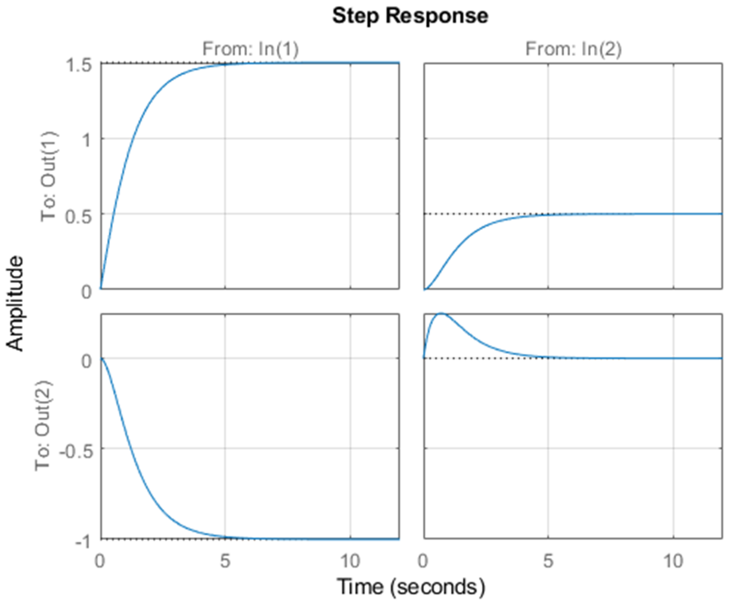The time history of the responses is shown in Figure 1. As apparent from Figure 1, $x_1(t)$ and $x_2(t)$ due to the first input are not in harmony in the sense that $x_1(t)$ increases positively and $x_2(t)$ increases negatively: an undesirable case in certain applications of mechanical and electrical systems.

For the two states, the reader can easily compare the initial values and steady values as given by Figure 1 with those obtained from the state time solutions given in Appendix A. This is done by substituting $t=0$ and $t=\infty$, respectively. A perfect match.

The next step is to control the system preserving the eigenvalues $-1$ and $-2$ but changing the closed loop eigenvectors $W_K$ to a new arbitrary one, say, $W_K=\left[\begin{array}{cc}1& 1\\ 2& 4\end{array}\right]$. This results in a left-eigenvector matrix.

$$Q_{\hspace{0.17em}K}{}^T=W_K{}^{-1}=\left[\begin{array}{cc}2& -0.5\\ -1& 0.5\end{array}\right]$$

(58)

Using either (54) or (55)

$$K=B^{-1}*({\Lambda }_K-A)=\left[\begin{array}{cc}0& -1.5\\ 6& 0\end{array}\right]\Rightarrow A_K=A+BK=\left[\begin{array}{cc}0& -0.5\\ 4& -3\end{array}\right]={\Lambda }_K$$

(59)

as expected. The closed loop system matrix $A_{\hspace{0.17em}K}$ has $-1$ and $-2$ as closed loop eigenvalues, but now with an alternative set of associated eigenvectors; those given by $W_K$.

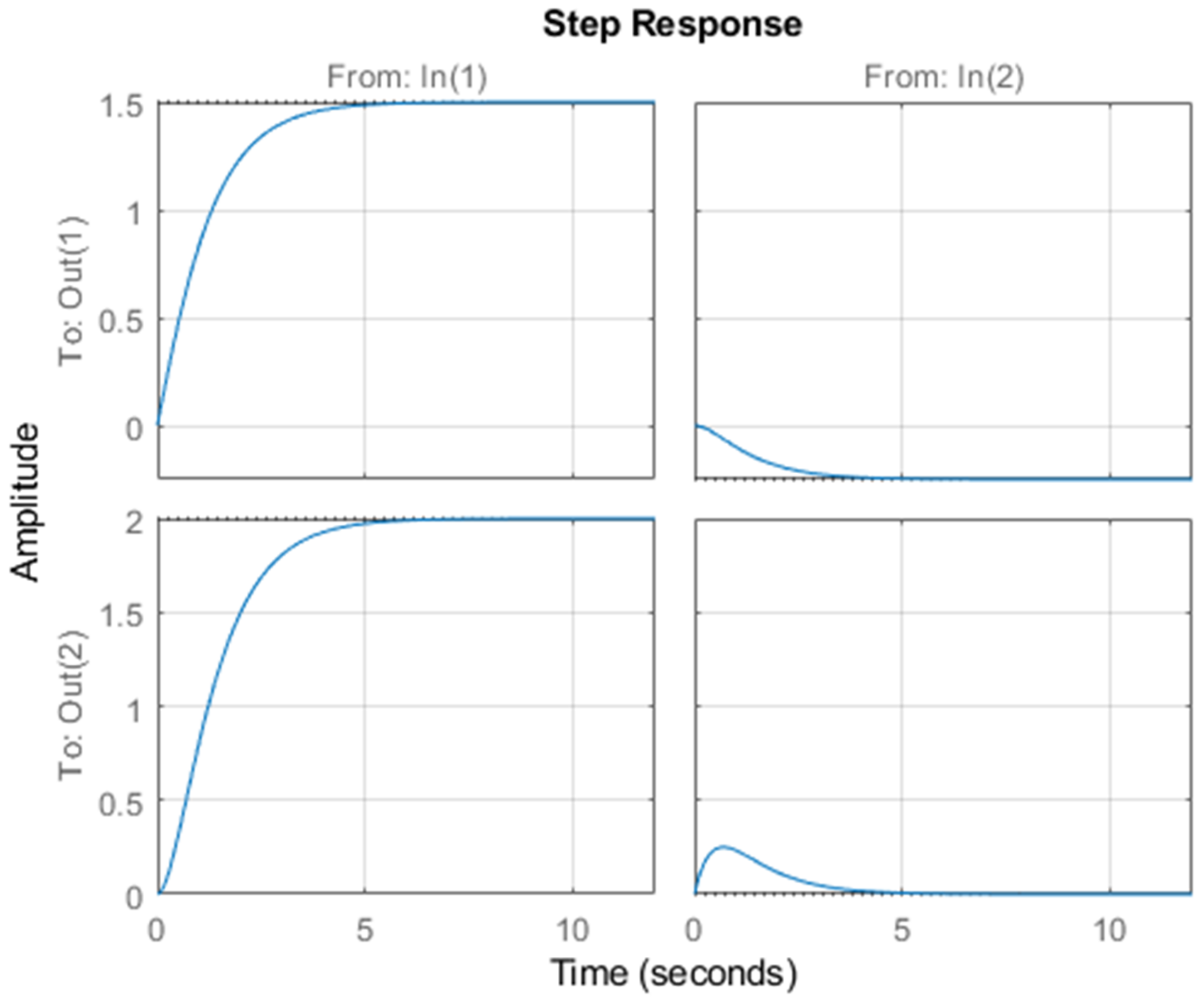
The same calculations are repeated for the closed loop system using the new $W_K$ and $Q_{\hspace{0.17em}K}{}^{\hspace{0.17em}T}$. The calculations are presented at the end of Appendix A. MATLAB is used once more to do the simulation for the closed loop system. The time response is presented in Figure 2, which shows a different time response resulting from the change in the eigenvectors (note that the eigenvalues are invariant). Due to the first input, both $x_1(t)$ and $x_2(t)$ are now increasing in harmony in contrast to their behavior due to the original set of open loop eigenvectors, a virtue attributed to the new set of closed loop eigenvectors. This value is attributed to the use of eigenstructure assignment.

The open loop eigenvalues are retained.

Example 2

Munro, ref. [37] considered a linearized time-scaled open loop unstable chemical reactor given by

$$\stackrel{•}{x}=\left[\begin{array}{cccc}1.38& -0.2077& 6.715& -5.676\\ -0.5814& -4.29& 0& 0.675\\ 1.067& 4.273& -6.654& 5.893\\ 0.048& 4.273& 1.343& -2.104\end{array}\right]x+\left[\begin{array}{ll}0\hfill & 0\hfill \\ 5.679\hfill & 0\hfill \\ 1.136\hfill & -3.146\hfill \\ 1.136\hfill & 0\hfill \end{array}\right]u$$

(60)

In our case, for the sake of demonstration, it is desired to assign the following four eigenvalues: −3 ± 8.5i, −0.7, and −6. These values are an approximation to the eigenvalues of the $A$ matrix of a model used in [37].

Throughout the examples, 5 decimal significant digits are displayed as given by MATLAB format short. To display 15 digits, format long can be used. With both formats, MATLAB employs number rounding. By default, it uses double precision arithmetic.

Using (20), which is related to the adjugate method.

$$w_C=adj((-3+8.5i)I_4-A)B=\left[\begin{array}{ll}0.1459+0.2484i\hfill & 0.6432+0.1331i\hfill \\ 0.9405 -4.9453i\hfill & -0.0131+0.0802i\hfill \\ -2.6218 - 0.8417i\hfill & -0.9188+2.0822i\hfill \\ -2.6516 - 0.8418i\hfill & 0.3808+0.1024i\hfill \end{array}\right]\times {10}^3$$

Considering the second eigenvector within $w_C$ to get $w_1$, $w_2$, $z_1$, and $z_2$, i.e.,

$$w_{12}=adj((-3+8.5i)I_4-A)B\left[\begin{array}{c}0\\ 1\end{array}\right]=\left[\begin{array}{c}1.6432+0.1331i\\ -0.0131+0.0802i\\ -0.9188+2.0822i\\ 0.3808+0.1024i\end{array}\right]\times {10}^3$$

(61)

Hence,

$$w_1=real(w_{12})=\left[\begin{array}{c}1643.2\\ -13.1\\ -918.8\\ 380.8\end{array}\right], w_2=imag(w_{12})=\left[\begin{array}{c}133.1\\ 80.2\\ 2082.2\\ 102.4\end{array}\right]$$

(62)

According to (21), the $z_C$ accompanying $w_{12}$ is

$$z_C=\left|(-3+8.5i)I_4-A\right|\left[\begin{array}{c}0\\ 1\end{array}\right]=\hspace{0.17em}\left[\begin{array}{c}0\\ 7945.6+409.78i\hspace{0.17em}\end{array}\right]$$

(63)

Hence,

$$z_1=real(z_C)=\left[\begin{array}{c}0\\ 7945.6\end{array}\right], z_2=imag(z_C)=\left[\begin{array}{c}0\\ 409.78\end{array}\right]$$

(64)

To simplify arithmetic, one can employ the real and imaginary parts of the pair $(w_i\hspace{0.17em},\hspace{0.17em}{z}_i)$ and avoid complex number manipulation. To assign $-3\pm 8.5i$, real number arithmetic is only used in the determination of $K$ as justified below.

For a general fourth order system, to simplify matters; parts related to the complex eigenvalues and eigenvectors are only accentuated. Let $W=W_R+i\hspace{0.17em}{W}_I$ and $Z=Z_R+i\hspace{0.17em}{Z}_I$ be associated with a generic eigenvalue say $\sigma +i\hspace{0.17em}\omega$, then,

$$K=\left[\begin{array}{cccc}\cdots & Z_R+i\hspace{0.17em}{Z}_I& Z_R-i\hspace{0.17em}{Z}_I& \cdots \end{array}\right]{\left[\begin{array}{cccc}⋮& W_R+i\hspace{0.17em}{W}_I& W_R-i\hspace{0.17em}{W}_I& ⋮\end{array}\right]}^{\hspace{0.17em}-1}$$

(65)

$$K=\left[\begin{array}{cccc}\cdots & Z_R& \hspace{0.17em}{Z}_I& \cdots \end{array}\right]\hspace{0.17em}\hspace{0.17em}\hspace{0.17em}\left[\begin{array}{cccc}1& & & \\ & 1& 1& \\ & i& -i& \\ & & & 1\end{array}\right]\hspace{0.17em}\hspace{0.17em}\hspace{0.17em}{\left(\left[\begin{array}{cccc}⋮& W_R& \hspace{0.17em}{W}_I& ⋮\end{array}\right]\hspace{0.17em}\hspace{0.17em}\hspace{0.17em}\left[\begin{array}{cccc}1& & & \\ & 1& 1& \\ & i& -i& \\ & & & 1\end{array}\right]\hspace{0.17em}\hspace{0.17em}\right)}^{\hspace{0.17em}-1}$$

$$K=\left[\begin{array}{cccc}\cdots & Z_R& \hspace{0.17em}{Z}_I& \cdots \end{array}\right]\left[\begin{array}{cccc}1& & & \\ & 1& 1& \\ & i& -i& \\ & & & 1\end{array}\right]{\left[\begin{array}{cccc}1& & & \\ & 1& 1& \\ & i& -i& \\ & & & 1\end{array}\right]}^{\hspace{0.17em}-1}{\left(\left[\begin{array}{cccc}⋮& W_R& \hspace{0.17em}{W}_I& ⋮\end{array}\right]\right)}^{\hspace{0.17em}-1}$$

$$K=\left[\begin{array}{cccc}\cdots & Z_R& \hspace{0.17em}{Z}_I& \cdots \end{array}\right]{\left[\begin{array}{cccc}⋮& W_R& \hspace{0.17em}{W}_I& ⋮\end{array}\right]}^{-1}\hspace{0.17em}$$

(66)

i.e., we can avoid computations involving complex numbers and only involve real number arithmetic since $Z_R$, $Z_I$, $W_R$ and $W_I$ are all real.

To assign $-0.7$, one may use the first closed loop eigenvector, i.e., $w_3$ is given by

$$w_3=adj(-0.7I_4-A)B\left[\begin{array}{c}1\\ 0\end{array}\right]=\left[\begin{array}{c}213.2098\\ -39.6625\\ -597.4124\\ -627.1864\end{array}\right]$$

(67)

With associated

$$z_3=\left|-0.7I_4-A\right|\left[\begin{array}{c}1\\ 0\end{array}\right]=71.3018\left[\begin{array}{c}1\\ 0\end{array}\right]=\left[\begin{array}{c}71.3018\\ 0\end{array}\right]$$

(68)

To assign $-6$. For the sake of demonstration, one may use the second closed loop eigenvector associated with $-6$, i.e., $w_4$ is given by

$$w_4=adj(-6I_4-A)B\left[\begin{array}{c}0\\ 1\end{array}\right]=\left[\begin{array}{c}-120.2254\\ \hspace{0.17em}-41.4320\\ 132.0392\\ 1.4068\end{array}\right]$$

(69)

With associated

$$z_4=\left|-6I_4-A\right|\left[\begin{array}{c}0\\ 1\end{array}\right]=-121.8635\left[\begin{array}{c}0\\ 1\end{array}\right]=\left[\begin{array}{c}0\\ -121.8635\end{array}\right]$$

(70)

Using (9),

$$K_1=\left[\begin{array}{cccc}{z}_1& z_2& z_3& z_4\end{array}\right]\hspace{0.17em}{\left[\begin{array}{cccc}{w}_1& w_2& w_3& w_4\end{array}\right]}^{\hspace{0.17em}-1}$$

(71)

$$K_1=\left[\begin{array}{llll}0.0274\hfill & -0.0641\hfill & 0.0059\hfill & -0.1060\hfill \\ 4.4156\hfill & -9.2451\hfill & 0.1762\hfill & 1.9179\hfill \end{array}\right]$$

(72)

Executing the MATLAB command “ $\gg eig\left(A+B*K\right)$” verifies the assignment of the four eigenvalues.

Suppose now that the eigenvectors associated with the two eigenvalues $-0.7$ and $-6$ are to be shaped. The ratio of the first to the fourth entries of the shaped closed loop eigenvector pertinent to −0.7 is a ratio of 2:1. The ratio of the second to the third entries of the shaped closed loop eigenvector pertinent to −6 is a ratio of 3:5. Relevant is remark iv in Section 5.

Using (20), the two eigenvectors associated with $w_3$ are

$$w_3=\left[\begin{array}{ll}213.2098 \hfill & 41.13789\hfill \\ -39.6625\hfill & 8.5490\hfill \\ -597.4124\hfill & 55.9057\hfill \\ -627.1864\hfill & 80.9017\hfill \end{array}\right]$$

(73)

then $M_3$ is calculated as follows (pick first and fourth rows of $w_3$).

$$\left[\begin{array}{cc}213.2098& 41.1379\\ -627.1864& 80.9017\end{array}\right]M_3=\left[\begin{array}{c}2\\ 1\end{array}\right]\Rightarrow M_3=\left[\begin{array}{c}0.0028\\ 0.0341\end{array}\right]$$

(74)

Consequently,

$$w_{3s}=w_3{M}_3=\left[\begin{array}{l}2\\ 0.1803\\ 0.2313\\ 1\end{array}\right]\hspace{0.17em}\hspace{0.17em}\hspace{0.17em};\hspace{0.17em}\hspace{0.17em}{z}_{3\hspace{0.17em}s}=\left[\begin{array}{cc}71.3018& 0\\ 0& 71.3018\end{array}\right]M_3=\left[\begin{array}{c}0.1999\\ 2.4307\end{array}\right]$$

(75)

The two eigenvectors associated with $w_4$ are

$$w_4=\left[\begin{array}{ll}58.3418\hfill & -120.2254\hfill \\ 615.5087\hfill & -41.4320\hfill \\ -453.9891 \hfill & 132.0392\hfill \\ -483.7589\hfill & 1.4068\hfill \end{array}\right]$$

(76)

then $M_4$ is calculated as follows (pick second and third rows of $w_4$).

$$\left[\begin{array}{cc}615.5087& -41.4320\\ -453.9891& 132.0392\end{array}\right]M_4=\left[\begin{array}{c}3\\ 5\end{array}\right]\Rightarrow M_4=\left[\begin{array}{c}0.0097\\ 0.0711\end{array}\right]$$

(77)

Finally,

$$w_{4s}=w_4{M}_4=\left[\begin{array}{l}-7.9816\\ 3\\ 5\\ -4.5723\end{array}\right]\hspace{0.17em}\hspace{0.17em};\hspace{0.17em}\hspace{0.17em}{z}_{4\hspace{0.17em}s}=\left[\begin{array}{cc}-121.8635& 0\\ 0& -121.8635\end{array}\right]M_4=\left[\begin{array}{c}-1.1770\\ -8.6615\end{array}\right]$$

(78)

Using (9),

$$K_2=\left[\begin{array}{cccc}{z}_1& z_2& z_{3s}& z_{4s}\end{array}\right]{\left[\begin{array}{cccc}{w}_1& w_2& w_{3s}& w_{4s}\end{array}\right]}^{\hspace{0.17em}-1}$$

(79)

$$K_2=\left[\begin{array}{llll}-0.1028\hfill & -0.0170\hfill & -0.0130\hfill & 0.4114\hfill \\ 8.2297\hfill & -2.5605\hfill & 0.4413\hfill & -13.6691\hfill \end{array}\right]$$

(80)

This is a different $K$ from that in (72), assigning the same eigenvalues, but different eigenvectors. The combined influence of the old set of eigenvalues with the newly shaped eigenvectors will yield a different time response.

Example 3

Consider the unstable system.

$$\stackrel{•}{x}=\left[\begin{array}{cccc}-5& 3& 3& 0\\ -6& 3& 4& 0\\ 0& 1& 0& 1\\ 0& 0& 0& -3\end{array}\right]x+\left[\begin{array}{c}1\\ 0\\ 0\\ 1\end{array}\right]u$$

(81)

It is required to assign $-2\pm i$, $-5$, and $-5$. The open loop characteristic polynomial is.

$$z=\left|\lambda I_4-A\right|={\lambda }^4+5{\lambda }^3+5{\lambda }^2-5\lambda -6$$

(82)

To assign the two eigenvalues $-2\pm i$, calculations for one eigenvalue say $-2+i$ suffices. Using (20).

$$w_C=adj((-2+i)I_4-A)B=\left[\begin{array}{c}9+i\\ 12+10i\\ -4-8i\\ 4+2i\end{array}\right]$$

(83)

Hence,

$$w_1\hspace{0.17em}=\hspace{0.17em}real(w_C)=\left[\begin{array}{c}9\\ 12\\ -4\\ 4\end{array}\right]\hspace{0.17em}\hspace{0.17em}\hspace{0.17em}\hspace{0.17em}\hspace{0.17em},\hspace{0.17em}\hspace{0.17em}\hspace{0.17em}\hspace{0.17em}\hspace{0.17em}{w}_2=imag(w_C)=\left[\begin{array}{c}1\\ 10\\ -8\\ 2\end{array}\right]$$

(84)

Using (21),

$$z(-2+i)\hspace{0.17em}\hspace{0.17em}=\hspace{0.17em}\hspace{0.17em}2+6i\hspace{0.17em}\hspace{0.17em}\hspace{0.17em}\Rightarrow \hspace{0.17em}\hspace{0.17em}\hspace{0.17em}{z}_1=\hspace{0.17em}\hspace{0.17em}\hspace{0.17em}real(z_C)\hspace{0.17em}\hspace{0.17em}=\hspace{0.17em}\hspace{0.17em}2\hspace{0.17em}\hspace{0.17em},\hspace{0.17em}\hspace{0.17em}\hspace{0.17em}{z}_2=\hspace{0.17em}\hspace{0.17em}imag(z_C)\hspace{0.17em}\hspace{0.17em}=\hspace{0.17em}\hspace{0.17em}6$$

(85)

To assign $-5$ and $-5$

$$w_3=adj(-5I_4-A)B=\left[\begin{array}{c}-84\\ -78\\ 30\\ -72\end{array}\right]\hspace{0.17em}\hspace{0.17em}\hspace{0.17em}\hspace{0.17em}\hspace{0.17em},\hspace{0.17em}\hspace{0.17em}\hspace{0.17em}\hspace{0.17em}\mathrm{and}\hspace{0.17em}\hspace{0.17em}\hspace{0.17em}\hspace{0.17em}{z}_3=z(-5)=144$$

(86)

Since $-5$ is a repeated eigenvalue, one way to determine $w_4$ and $z_4$ is using the first order derivative of both $w_3$ and $z_3$ with respect to $\lambda$ as given by (44). MATLAB was used to do that symbolically. In which case, the closed loop eigenvectors in terms of a general $\lambda$ are given by.

$$w\hspace{0.17em}(\lambda )=\left[\begin{array}{c}{\lambda }^3-10\lambda -9\\ -6{\lambda }^2-14\lambda +2\\ {\lambda }^2-4\lambda -15\\ {\lambda }^3+2{\lambda }^2-\lambda -2\end{array}\right]$$

(87)

To validate (87), $w_3=w\hspace{0.17em}(-5\hspace{0.17em})={\left[\begin{array}{cccc}-84& -78& 30& -72\end{array}\right]}^{\hspace{0.17em}T}$ as already obtained using the adjugate method, using (87) to determine $w_4$ where $w_4$ is the first generalized eigenvector pertinent to $-5$. Hence, use (44) to get the first derivative.

$$w_4={\left.\frac{dw(\lambda )}{d\lambda }\hspace{0.17em}\hspace{0.17em}\right|}_{\hspace{0.17em}\hspace{0.17em}\lambda \hspace{0.17em}=\hspace{0.17em}-\hspace{0.17em}5}={\left.\left[\begin{array}{c}3{\lambda }^2-10\\ -12\lambda -14\\ 2\lambda -4\\ 3{\lambda }^2+4\lambda -1\end{array}\right]\hspace{0.17em}\hspace{0.17em}\right|}_{\hspace{0.17em}\hspace{0.17em}\lambda \hspace{0.17em}=\hspace{0.17em}\hspace{0.17em}-\hspace{0.17em}5}=\left[\begin{array}{c}65\\ 46\\ -14\\ 54\end{array}\right]$$

(88)

$$z_4=\hspace{0.17em}\hspace{0.17em}{\left.\frac{dz}{d\lambda }\hspace{0.17em}\right|}_{\lambda =-5}={\left.4{\lambda }^3+15{\lambda }^2+10\lambda -5\hspace{0.17em}\right|}_{\lambda =-5}\Rightarrow z_4=-180\hspace{0.17em}\hspace{0.17em}\hspace{0.17em}$$

(89)

Thus, using (9),

$$\begin{gathered} K_1=\left[\begin{array}{cccc}{z}_1& z_2& z_3& z_4\end{array}\right]\hspace{0.17em}{\left[\begin{array}{cccc}{w}_1& w_2& w_3& w_4\end{array}\right]}^{\hspace{0.17em}-1} \\ {K}_1=\left[\begin{array}{cccc}2& 6& 144& -180\end{array}\right]{\left[\begin{array}{cccc}9& 1& -84& 65\\ 12& 10& -78& 46\\ -4& -8& 30& -14\\ 4& 2& -72& 54\end{array}\right]}^{\hspace{0.17em}-1} \\ {K}_1=\left[\begin{array}{cccc}-16.4& 16.6& 19.8& 7.4\end{array}\right] \end{gathered}$$

(90)

Once more, for the sake of exercise and for checking the answer through an alternative approach, the eigenvectors associated with $-5$ are now determined using the traditional null space method.

Having obtained $w_3$ using the adjugate method, we now use (52) bearing in mind that $z_{3M\hspace{0.17em}r}=1$ and

$$\begin{array}{l}{w}_3=w_{3M\hspace{0.17em}r}=w_{3adj}/z_{3adj}\\ \hspace{0.17em}\hspace{0.17em}\hspace{0.17em}\hspace{0.17em}\hspace{0.17em}\hspace{0.17em}\hspace{0.17em}={\left[\begin{array}{cccc}-84& -78& 30& -72\end{array}\right]}^{\hspace{0.17em}T}/144=\left[\begin{array}{cccc}-0.5833& -0.5417& 0.2083& -0.05\end{array}\right]\end{array}$$

(91)

Equation (91) is now used to determine the null space solution for the $w_4$ generalized eigenvector using (40). If $\mu \ne 1$, the solution vector is divided by $\mu$, i.e.,

$$\left[\begin{array}{lll}{\lambda }_3{I}_4\hfill & -B\hfill & -w_3\hfill \end{array}\right]\left[\begin{array}{l}{w}_4\hfill \\ z_4\hfill \\ \mu \hfill \end{array}\right]=0_{4\times 1}$$

(92)

$$\left[\begin{array}{llllll}0\hfill & -3\hfill & -3\hfill & 0\hfill & -1\hfill & -0.5833\hfill \\ 6\hfill & -8\hfill & -4\hfill & 0\hfill & 0\hfill & -0.5417\hfill \\ 0\hfill & -1\hfill & -5\hfill & -1\hfill & 0\hfill & 0.2083\hfill \\ 0\hfill & 0\hfill & 0\hfill & -2\hfill & -1\hfill & -0.05\hfill \end{array}\right]\left[\begin{array}{l}{w}_4\hfill \\ z_4\hfill \\ \mu \hfill \end{array}\right]=0_{4\times 1}$$

(93)

Using MATLAB $null(\hspace{0.17em}\left[\begin{array}{ccc}-5*eye(4)-A& -B& -w_3\end{array}\right],\prime r\prime \hspace{0.17em})$,

$$\left[\begin{array}{l}{w}_4\hfill \\ z_4\hfill \\ \mu \hfill \end{array}\right]=\left[\begin{array}{ll}-0.5833\hfill & 0.2778\\ -0.5417& 0.3576\\ 0.208& -0.1632\\ -0.5& 0.25\\ 1\hfill & 0=z_4\hfill \\ 0\ne \hspace{0.17em}\mathrm{nonzero},& 1=\mu \ne 0\\ \mathrm{vector}\hspace{0.17em}\hspace{0.17em}\mathrm{rejected}& \mathrm{vector}\hspace{0.17em}\hspace{0.17em}\mathrm{accepted}\end{array}\right]\hspace{0.17em},\hspace{0.17em}\hspace{0.17em}\mathrm{hence},\hspace{0.17em}\hspace{0.17em}{w}_4=\left[\begin{array}{c}0.2778\\ 0.3576\\ -0.1632\\ 0.25\end{array}\right]\hspace{0.17em}\hspace{0.17em},\hspace{0.17em}\hspace{0.17em}{z}_4=0\hspace{0.17em},\hspace{0.17em}\hspace{0.17em}\mu =1$$

(94)

Two solutions are obtained. The one ending with a nonzero element for $\mu$ is adopted for $w_4$. It turns out that $\mu$ already equals $1$, so no need for normalization. Moreover, the other solution given by the first column is $w_3$. It cannot be used as it results in a singular eigenvector matrix having no inverse. Hence,

$$K_2=\left[\begin{array}{cccc}2& 6& 1& 0\end{array}\right]{\left[\begin{array}{cccc}{w}_1& w_2& w_3& w_4\end{array}\right]}^{\hspace{0.17em}-1}=\hspace{0.17em}\left[\begin{array}{cccc}-16.4& 16.6& 19.8& 7.4\end{array}\right]$$

(95)

The same answer as in (90) as it should be since the system is single input and controllable.

Addendum

To assign four repeated eigenvalues on the imaginary axis, they should have the form $\pm \omega \hspace{0.17em}i$ and $\pm \omega \hspace{0.17em}i$. This is due to the conjugacy of the eigenvalues of real-number matrices. For the sake of simplicity, let the eigenvalues be i, i, −i, and –i. In this case, the adjugate method requires determination of an eigenvector and its derivative for one eigenvalue say i. Utilizing their conjugates, the eigenvectors for the –i eigenvalues are determined. Using the adjugate method together with MATLAB with $\lambda =\omega \hspace{0.17em}i$

$$w_1=\hspace{0.17em}{\left.\left[\begin{array}{c}{\lambda }^3-10\lambda -9\\ -6{\lambda }^2-14\lambda +2\\ {\lambda }^2-4\lambda -15\\ {\lambda }^3+2{\lambda }^2-\lambda -2\end{array}\right]\right|}_{\lambda =\omega \hspace{0.17em}i}=\hspace{0.17em}\hspace{0.17em}\hspace{0.17em}\left[\begin{array}{c}-9+(-{\omega }^3-10\omega )\hspace{0.17em}i\\ 2+6{\omega }^2-14\omega \hspace{0.17em}i\\ -15-{\omega }^2-4\omega \hspace{0.17em}i\\ -2-2{\omega }^2+(-{\omega }^3-\omega )\hspace{0.17em}i\end{array}\right]$$

(96)

and

$$\hspace{0.17em}{w}_2=w_d=\frac{dw}{d\lambda }={\left.\left[\begin{array}{c}3{\lambda }^2-10\\ -12\lambda -14\\ 2\lambda -4\\ 3{\lambda }^2+4\lambda -1\end{array}\right]\right|}_{\lambda =\omega \hspace{0.17em}i}=\hspace{0.17em}\hspace{0.17em}\hspace{0.17em}\left[\begin{array}{c}-10-3{\omega }^2\\ -14-12\omega \hspace{0.17em}i\\ -4-2\omega \hspace{0.17em}i\\ -1-3{\omega }^2+4\omega \hspace{0.17em}i\end{array}\right]$$

(97)

The remaining two eigenvectors are $w_3=\overline{w_1}$ and $w_4=\overline{w_2}$,where the bar indicates complex conjugacy.

The characteristic polynomial and its derivative at $\lambda =\omega \hspace{0.17em}i\hspace{0.17em}$ are needed, where

$$p(\lambda )={\lambda }^4+5{\lambda }^3+5{\lambda }^2-5\lambda -6$$

(98)

$${\left.z_1=p(\lambda )\right|}_{\lambda =\omega \hspace{0.17em}i}={\left.\left|\lambda \hspace{0.17em}{I}_n-A\right|\right|}_{\lambda =\omega \hspace{0.17em}i}\hspace{0.17em}=\hspace{0.17em}-6-5{\omega }^2+{\omega }^4+(-5{\omega }^3\hspace{0.17em}-5\omega )\hspace{0.17em}i$$

$${\left.z_2=p^{(1)}(\lambda )\right|}_{\lambda =\omega \hspace{0.17em}i}=-5-15{\omega }^2+(-4{\omega }^3+10\omega \hspace{0.17em})\hspace{0.17em}i$$

(99)

Similarly,

$$z_3=\overline{z_1} \mathrm{and} z_4=\overline{z_2}$$

(100)

Hence, when $\omega$ = 1

$$Z=\hspace{0.17em} \hspace{0.17em}\left[\begin{array}{cccc}-10 -10i& -20+6i& -10+10i& -20 - 6i\end{array}\right]$$

(101)

$$W=\left[\begin{array}{cccc}-9 -11i& -13& -9+11i& -13\\ 8 -14i& -14 -12i& 8+14i& \hspace{0.17em}-14+12i\\ -16 - 4i& -4+2i& -16+4i& -4 - 2i\\ -4 - 2i& -4+4i& -4+2i& \hspace{0.17em}-4 - 4i\end{array}\right]$$

(102)

$$\begin{array}{ll}K=Z\hspace{0.17em}{W}^{-1}& =\left[\begin{array}{cccc}-706& 349& 367& 931\end{array}\right]/45\\ & =\left[\begin{array}{cccc}-15.6889& 7.7556& 8.1556& 20.6889\end{array}\right]\hspace{0.17em}\end{array}$$

(103)

resulting in the assignment of i, i, −i, −i as closed loop eigenvalues on the imaginary axis.

In addition, a well-known and interesting problem in discrete systems design is that of dead-beat control, where all $n$ eigenvalues are located at the origin. In such case of repeated eigenvalue assignment, we need to differentiate the eigenvector as determined by the adjugate method three times and evaluating all $n$ eigenvectors at $\lambda =0$. Thus, the calculations are considerably simplified. The same is done to the open loop characteristic polynomial and three of its derivatives at $\lambda =0$ to get $Z$.

Doing so, we get

$$W=\left[\begin{array}{cccc}-9& -10& 0& 6\\ 2& -14& -12& 0\\ -15& -4& 2& 0\\ -2& -1& 4& 6\end{array}\right]$$

(104)

$$\begin{array}{ll}K=Z\hspace{0.17em}\hspace{0.17em}{W}^{\hspace{0.17em}-1}& =\left[\begin{array}{cccc}-469& 233.5& 238& 694\end{array}\right]/45\\ & =\left[\begin{array}{cccc}-10.4222& 5.1889 & 5.2889& 15.4222\end{array}\right]\end{array}$$

(105)

Example 4

In this example we consider a model of a practical electrical system; that of a DC motor. DC motors are widely used in control applications such as robotics, tape drives and autotronics. The motor has many advantages, among which are high startup torque and fast response times to starting, stopping, reversing, and acceleration. In addition, to easy control of speed with moderate voltage or current inputs.

Almost any book on control systems goes through the modeling of an armature control DC motor to a certain degree of complexity [16,33,38]. We shall refer to a research paper [38] which tackles an armature controlled DC motor used in robotics. However, the model in that paper has been represented by a block diagram model. We take the liberty and derive a state space model of that motor. To do that, we replace $T_m$ by its equivalent $K_m{i}_a$, $T_d$ by $d$ for convenience, and adopt the following state variables assignment: $x_1$ for the angular displacement ($\theta$), $x_2$ for the angular velocity ($\omega$), and $x_3$ for the armature current ($i_a$). The output $y$ is the angular velocity $x_2$. The armature voltage is $u$ and the load disturbance is $d$.

We obtain the following state space model. It is a two-input, single output model.

$${\dot{x}}_1=x_2$$

(106)

$${\dot{x}}_2=-\frac{b}{J}{x}_2+\frac{K_m}{J}{x}_3-\frac{1}{J}d$$

(107)

$${\dot{x}}_3=-\frac{K_b}{L}{x}_2-\frac{R}{L}{x}_3+\frac{1}{L}u$$

(108)

$$y=\left[\begin{array}{ccc}0& 1& 0\end{array}\right]x$$

(109)

In matrix form,

$$\dot{x}=\left[\begin{array}{ccc}0& 1& 0\\ 0& -b/J& K_m/J\\ 0& -K_b/L& -R/L\end{array}\right]x+\left[\begin{array}{ll}0\hfill & \hspace{0.17em}\hspace{0.17em}\hspace{0.17em}0\hfill \\ 0\hfill & -1/J\hfill \\ 1/L\hfill & \hspace{0.17em}\hspace{0.17em}\hspace{0.17em}\hspace{0.17em}0\hfill \end{array}\right]\left[\begin{array}{c}u\\ d\end{array}\right]\hspace{0.17em}\hspace{0.17em}\hspace{0.17em}\hspace{0.17em}\hspace{0.17em}\hspace{0.17em}\hspace{0.17em},\hspace{0.17em}\hspace{0.17em}\hspace{0.17em}\hspace{0.17em}\hspace{0.17em}\hspace{0.17em}y=\left[\begin{array}{ccc}0& 1& 0\end{array}\right]x$$

(110)

where $J$ is the motor moment of inertia, $b$ is viscous friction coefficient, $K_m$ is motor constant, $K_b$ is back electromotive force coefficient, $R$ and $L$ are the armature resistance and inductance, respectively. Numerical values for these coefficients are not given in [38]. Therefore, for the sake of demonstration we use the following values which may pertain to an existing generic DC motor: (source: directindustory.com, 2011). They are: $\begin{array}{l}J=\hspace{0.17em}0.0211\hspace{0.17em}Kg.\hspace{0.17em}{m}^2\hspace{0.17em};\hspace{0.17em}\hspace{0.17em}b=0.002953\hspace{0.17em}\hspace{0.17em}N.\hspace{0.17em}m.\hspace{0.17em}s\hspace{0.17em}\hspace{0.17em};\hspace{0.17em}\hspace{0.17em}{K}_m=0.516\hspace{0.17em}\hspace{0.17em}N.\hspace{0.17em}m/A\hspace{0.17em}\hspace{0.17em}\hspace{0.17em}\\ K_b=1.25\hspace{0.17em}V.\hspace{0.17em}s/rad\hspace{0.17em}\hspace{0.17em};\hspace{0.17em}\hspace{0.17em}R=2.581\hspace{0.17em}\Omega \hspace{0.17em}\hspace{0.17em}\hspace{0.17em};\hspace{0.17em}\hspace{0.17em}\hspace{0.17em}L=0.0281\hspace{0.17em}\hspace{0.17em}\mathrm{H}\end{array}$.

Substituting the parameters listed above in (100), we get

$$\stackrel{•}{x}=\left[\begin{array}{ccc}0& 1& 0\\ 0& -0.1336& 23.3484\\ 0& -18.3630& -91.8505\end{array}\right]x+\left[\begin{array}{ll}0\hfill & 0\hfill \\ 0\hfill & -45.2489\hfill \\ 35.5872\hfill & 0\hfill \end{array}\right]u\hspace{0.17em}\hspace{0.17em}\hspace{0.17em},\hspace{0.17em}\hspace{0.17em}\hspace{0.17em}y=\left[\begin{array}{ccc}0& 1& 0\end{array}\right]x$$

(111)

The open loop eigenvalues are $\{\hspace{0.17em}0\hspace{0.17em},\hspace{0.17em}\hspace{0.17em}-5.0745\hspace{0.17em},\hspace{0.17em}\hspace{0.17em}-86.9097$. As we are concentrating on the speed control of such a motor, with no intention to control the position of the motor, we seek a controller which retains the zero eigenvalue. To speed up the system we choose closed loop eigenvalues which are almost two-folds of the open loop ones, say $\{\hspace{0.17em}0\hspace{0.17em},\hspace{0.17em}\hspace{0.17em}-10\hspace{0.17em},\hspace{0.17em}\hspace{0.17em}-200\}$. Using the adjugate method with eigenvector shaping, the procedure followed in Example 2 and in Example 3 is repeated.

In our design, a closed loop eigenvector $w_1={\left[\begin{array}{ccc}1& 0& 0\end{array}\right]}^{\hspace{0.17em}T}$ together with $z_1=0$ are associated with ${\lambda }_1=0$. The other two eigenvectors associated with ${\lambda }_2=-10$ and ${\lambda }_3=-200$ are shaped with ratios $\hspace{0.17em}2:-1$ and $1:-1$ between the second and third entries of $w_2$ and $w_3$, respectively.

To avoid any unnecessary repetition, the calculations needed are the same as those carried out in Example 2 and Example 3. We therefore content ourselves with the following final results.

$$\begin{gathered} Z=\left[\begin{array}{ccc}{z}_1& z_2& z_3\end{array}\right]=\left[\begin{array}{lll}0\hfill & -1.2680\hfill & 3.550\hfill \\ 0\hfill & -0.0799\hfill & 3.9010\hfill \end{array}\right] \\ W=\left[\begin{array}{ccc}{w}_1& w_2& w_2\end{array}\right]\hspace{0.17em}\hspace{0.17em}=\hspace{0.17em}\left[\begin{array}{ccc}1& -0.2& -0.005\\ 0& 2& 1\\ 0& -1& -1\end{array}\right] \end{gathered}$$

(112)

Consequently,

$$K=Z\hspace{0.17em}{W}^{\hspace{0.17em}-1}=\left[\begin{array}{lll}0\hfill & -48230\hfill & -8.3780\hfill \\ 0\hfill & -3.9810\hfill & -7.8820\hfill \end{array}\right]$$

(113)

Yielding

$$\stackrel{•}{x}=\left[\begin{array}{ccc}0& 1& 0\\ 0& -0.1336& 23.3484\\ 0& -18.3630& -91.8505\end{array}\right]x+\left[\begin{array}{ll}0\hfill & 0\hfill \\ 0\hfill & -45.2489\hfill \\ 35.5872\hfill & 0\hfill \end{array}\right]u\hspace{0.17em}\hspace{0.17em}\hspace{0.17em},\hspace{0.17em}\hspace{0.17em}\hspace{0.17em}y=\left[\begin{array}{ccc}0& 1& 0\end{array}\right]x$$

(114)

The steady state value due to a step input is [33],

$$y_{ss}=C\hspace{0.17em}{x}_{ss}=x_{2ss}=-A_M{}^{-1}\hspace{0.17em}{B}_v\hspace{0.17em}\hspace{0.17em},\hspace{0.17em}\hspace{0.17em}\hspace{0.17em}{B}_v=\left[\begin{array}{lll}0\hfill & 1\hfill & 0\hfill \\ 0\hfill & 0\hfill & 1\hfill \end{array}\right]B\hspace{0.17em}\left[\begin{array}{cc}U& 0\\ 0& d\end{array}\right]$$

(115)

were $y_{ss}$ and $x_{ss}$ are steady state values. $A_M$ and $B_v$ as defined in (114) and (115). The armature voltage is $U$ and $d$ is the disturbing value.

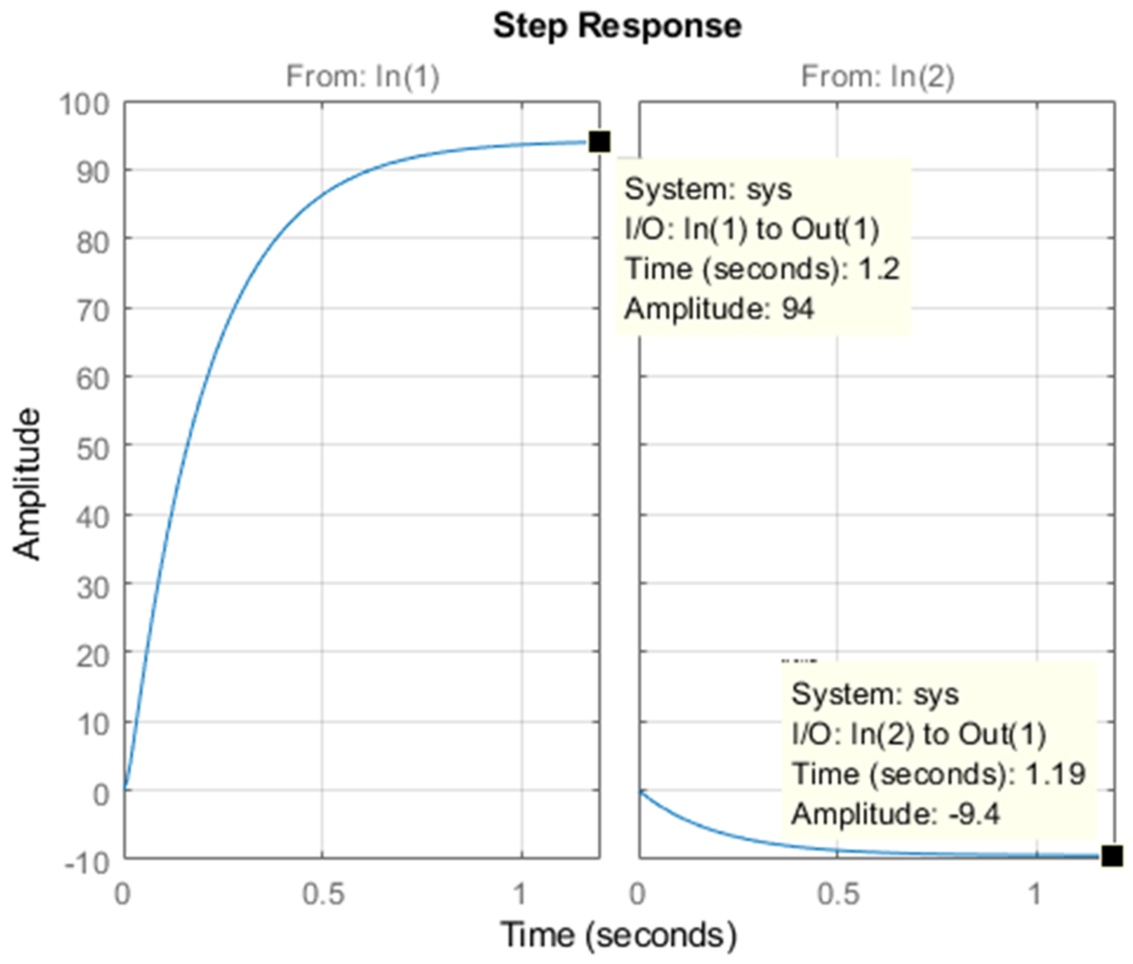
MATLAB $step$ function [33] gives a time record of the outputs due to an excitation of a single input at a time. The time history of the motor output is shown in Figure 3.

The open loop response is depicted in Figure 3, which shows the motor steady state speed reaching 94 rpm due to a 50 V armature voltage and −9.4 rpm due to a unit step disturbance. Both reached within a time interval of about 1.2 s. Using (115), the exact calculated steady state values are 94.2026 rpm and −9.4239 rpm, respectively, where $A_M$ is now obtained from (111).

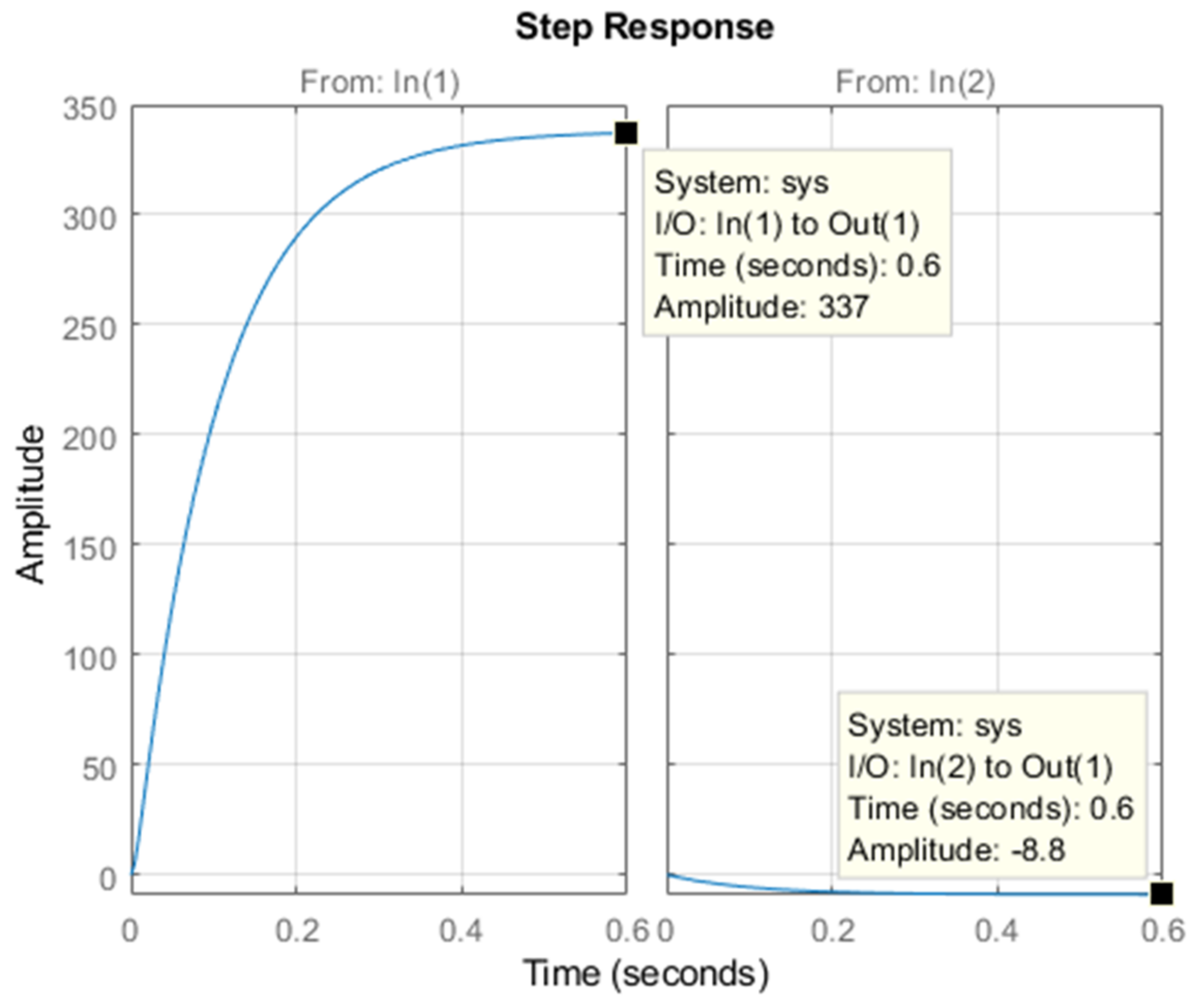
The closed loop system response as a result of $K$ as in (113) is depicted in Figure 4. It shows the motor steady state speed reaching 337 rpm due to a 50 V armature voltage and −8.8 rpm due to a unit step disturbance. Both were reached within a time interval of about 0.6 s. This gives a clear indication of the effect of feedback in increasing the motor speed and in reducing the time to reach the steady state. Using (115), the exact calculated steady state values are 338.0783 rpm and −8.8235 rpm, respectively.

The example undoubtedly demonstrates the role played by the eigenvectors in shaping the system response. Every choice of the ratios of the closed loop eigenvector entries makes a difference on the final speed and the settling time. Experimenting with alternatives values for the ratios proves that. Note that the feedback matrix $K$, the settling time, and the speed will differ every time a ratio is changed, though the closed loop eigenvalues remain invariant at $0\hspace{0.17em},\hspace{0.17em}-10\hspace{0.17em},\hspace{0.17em}-200$. That is due to the influence of the closed loop eigenvectors in shaping the system response both in the transient and the steady state.

The program used to do the calculations and the simulations acquired for Example 4 are listed in Appendix B. It is provided for validating the results and for readers’ experimentation with alternative ratios of eigenvectors entries.

10. Conclusions

The null space method is a general purpose method, though it is computationally more demanding compared to the adjugate method. Moreover, it is not a direct method for the individual determination of the admissible pair $w$ and $z$.

The adjugate method proves a worthy method for exposing internal structures within the eigenstructure assignment problem. With regard to the lumped solution as given by traditional methods, the adjugate method offers decoupled solutions for each component of the admissible pair $(w,z)$, which is considered advantageous. A new feature is highlighted and emphasized regarding a fundamental role played by the open loop characteristic polynomial. This point is overshadowed by other methods related to eigenstructure as well as to methods of eigenvalue assignment in general.

Additional insight has been gained by the use of the adjugate method. For the case of assigning a new eigenvalue not that of $A$: $z$ has been proved to be nonzero and not influenced by the system input matrix $B$, regardless of a system being controllable or otherwise.

The adjugate method attests itself as a formula-based method. It is explicit and independently determines both $w_i$ and $z_i$. This is considered an advantage since closed forms methods are pedagogically favorable. Such independent determination of the admissible pair can be looked upon as a form of parallelism which is always desirable.

Special forms ease calculations both in analysis and in design through their readily available information such as the characteristic polynomial and the stability of the open loop system in certain cases. Besides, the columns and rows of the adjugate of ${\lambda }_{\hspace{0.17em}i}{I}_n-A$ represent the right and left eigenvectors and its trace determines the derivative of the characteristic polynomial with respect to $\lambda$. All such features ease analysis and design.

The four examples presented have illustrated the various concepts and notions with the help of MATLAB which proves an admirable software when it comes to control theory studies. MATLAB proves very helpful when it comes to complex number calculations and visualization in addition to its symbolic calculations.

As for shortcomings of the adjugate method, numerical issues may arise as the dimensions of the system get higher; however, this shortcoming also applies to the traditional method. In this case, more numerically efficient methods such as the Faddeev–Leverrier’s algorithm for determining the matrix adjugate may be considered [39]. Special matrix forms other than companion forms are also worth considering in forthcoming studies.

Future works should consider methods which simplify assignment issues related to partial eigenstructure assignment for both cases of controllable and uncontrollable systems, for both single-input and multi-input systems.

References

1. Moore, B.C. On the Flexibility Offered by State Feedback in Multivariable Systems Beyond Closed Loop Eigenvalue Assignment. IEEE Trans. Autom. Control 1976, 21, 689–692. [Google Scholar] [CrossRef]
2. Klein, G.; Moore, B.C. Eigenvalue Generalized eigenvector assignment with state feedback. IEEE Trans. Autom. Control 1977, 22, 140–141. [Google Scholar] [CrossRef]
3. Liu, G.P.; Patton, R.J. Eigenstructure Assignment for Control System Design; John Wiley & Sons: New York, NY, USA, 1998. [Google Scholar]
4. Liu, G.P.; Patton, R.J. Eigenstructure Assignment Toolbox for Use with MATLAB; Pacilantic International Ltd.: Oxford, UK, 1999. [Google Scholar]
5. White, B.A. Eigenstructure Assignment: A Survey. Proc. Inst. Mech. Eng. 1995, 209, 1–11. [Google Scholar] [CrossRef]
6. Andry, A.N.; Shapiro, E.Y.; Chung, J.C. Eigenstructure assignment for linear systems. IEEE Trans. Aerosp. Electron. Syst. 1983, 19, 711–728. [Google Scholar] [CrossRef]
7. Porter, B.; D’Azzo, J.J. Algorithm for the Synthesis of State-Feedback Regulators by Entire Eigenstructure Assignment. Electron. Lett. 1977, 13, 230–231. [Google Scholar] [CrossRef]
8. Porter, B. Eigenvalue assignment in linear multivariable systems by output feedback. Int. J. Control 1977, 25, 483–490. [Google Scholar] [CrossRef]
9. Porter, B.; D’Azzo, J.J. Closed loop eigenstructure assignment by state feedback in multivariable linear systems. Int. J. Control 1978, 27, 487–492. [Google Scholar] [CrossRef]
10. Porter, B.; D’Azzo, J.J. Algorithm for closed loop eigenstructure assignment by state feedback in multivariable linear systems. Int. J. Control 1978, 27, 943–947. [Google Scholar] [CrossRef]
11. Kautsky, J.; Nichols, N.; van Dooren, D.P. Robust Pole Assignment in Linear State Feedback. Int. J. Control 1985, 41, 1129–1155. [Google Scholar] [CrossRef]
12. Inman, D.J. Vibration with Control; John Wiley & Sons Ltd.: Chichester, UK, 2006. [Google Scholar]
13. Srinathkumar, S. Eigenstructure Control Algorithms: Application to Aircraft/Rotorcraft Handling Qualities Design; The Institution of Engineering and Technology IET 74: London, UK, 2011. [Google Scholar]
14. Littleboy, D.M. Numerical Techniques for Eigenstructure Assignment by Output Feedback in Aircraft Applications. Ph.D. Thesis, University of Reading, Reading, UK, December 1994. [Google Scholar]
15. D’azzo, J.J.; Houpis, C.H. Linear Control Systems: Analysis and Design, 4th ed.; McGraw-Hill: New York, NY, USA, 1995. [Google Scholar]
16. Houpis, C.H.; Sheldon, S.N. Linear Control System Analysis and Design with MATLAB, 6th ed.; CRC Press, Taylor & Francis Group: New York, NY, USA, 2014. [Google Scholar]
17. Gu, D.K.; Wang, R.Y.; Liu, Y.D.A. A parametric approach of partial eigenstructure assignment for high-order linear systems via proportional plus derivative state feedback. AIMS Math. 2021, 6, 11139–11166. [Google Scholar] [CrossRef]
18. Duan, G.R. Circulation algorithm for partial eigenstructure assignment via state feedback. Eur. J. Control 2019, 50, 107–116. [Google Scholar] [CrossRef]
19. Bernal, D.; Ulriksen, M.D. Output feedback in the design of eigenstructures for enhanced sensitivity. Mech. Syst. Signal Process. 2018, 112, 22–30. [Google Scholar] [CrossRef]
20. Rastgaar, M.; Ahmadian, M.; Southward, S. A review on eigenstructure assignment methods and orthogonal eigenstructure control of structural vibrations. Shock and Vibration. Shock Vib. 2009, 16, 555–564. [Google Scholar] [CrossRef]
21. Köthe, A.; Luckner, R. Applying Eigenstructure Assignment to Inner-Loop Flight Control Laws for a Multibody Aircraft. CEAS Aeronaut. J. 2022, 13, 33–43. [Google Scholar] [CrossRef]
22. Prewett, P. Foundation Mathematics for Science and Engineering Students; Springer: Berlin/Heidelberg, Germany, 2022. [Google Scholar]
23. Wikipedia. Adjugate Matrix. 2022. Available online: https://en.wikipedia.org/wiki/Adjugate_matrix (accessed on 1 October 2022).
24. Horn, R.A.; Johnson, C.R. Matrix Analysis, 2nd ed.; Cambridge University Press: Cambridge, MA, USA, 2013. [Google Scholar]
25. Brookes, M. The Matrix Reference Manual; Imperial College: London, UK, 2021; Available online: http://www.ee.imperial.ac.uk/hp/staff/dmb/matrix/intro.html (accessed on 30 September 2022).
26. Wikipedia. Kernel. Available online: https://en.wikipedia.org/wiki/Kernel_(linear_algebra) (accessed on 30 September 2022).
27. Lerner, D. Lecture Notes on Linear Algebra; Department of Mathematics, University of Kansas: Kansas, TX, USA, 2008; Available online: https://www-labs.iro.umontreal.ca/~grabus/courses/ift6760_files/LANotes.lerner.pdf (accessed on 30 September 2022).
28. Golub, G.H.; van Loan, C.F. Matrix Computations, 4th ed.; Johns Hopkins University Press: Baltimore, MD, USA, 2013. [Google Scholar]
29. Garcia, S.R.; Horn, R.A. Block Matrices in Linear Algebra. In PRIMUS: Problems, Resources, and Issues in Mathematics Undergraduate Studies; Taylor & Francis Group, LLC.: New York, NY, USA, 2020; Volume 30, pp. 285–306. [Google Scholar] [CrossRef]
30. Beezer, R.A. A First Course in Linear Algebra; Version 3.5.; University of Puget Sound, Congruent Press: Tacoma, WA, USA, 2015; Available online: https://open.umn.edu/opentextbooks/textbooks/5 (accessed on 30 September 2022).
31. MATLAB by Mathworks, Command: Compan. 2020. Available online: http://www.mathworks.com/help/control/ref/place.html (accessed on 1 October 2022).
32. Neamen, D.A. Microelectronics: Circuit Analysis and Design, 4th ed.; McGraw Hill: New York, NY, USA, 2010. [Google Scholar]
33. Ogata, K. Modern Control Engineering, 5th ed.; Prentice Hall: Hoboken, NJ, USA, 2010. [Google Scholar]
34. Chen, C.T. Linear System theory and Design, 4th ed.; Oxford University Press: Oxford, UK, 2013. [Google Scholar]
35. MATLAB by Mathworks. Command: Diff. Release R2022a. 2022. Available online: https://www.mathworks.com/help/symbolic/diff.html (accessed on 1 October 2022).
36. MATLAB by Mathworks. Command: Null. Release R2022a. 2022. Available online: https://www.mathworks.com/help/matlab/ref/null.html (accessed on 1 October 2022).
37. Munro, N. Design of Controller for an Open-Loop Unstable Multivariable System Using the Inverse Nyquist Array. Proc. Inst. Electr. Eng. 1972, 119, 1377–1382. [Google Scholar] [CrossRef]
38. Foldager, F.; Thomsen, D.; Li, H.; Frederiksen, K.; Andersen, A.; Zhang, X. Electrical-Mechanical Dynamic Modelling and Testing of a Lightweight-Link Robot Manipulator. In Proceedings of the World Congress on Mechanical, Chemical, and Material Engineering (MCM 2015), Barcelona, Spain, 20–21 July 2015; Paper No. 251. pp. 251-1–259-9. [Google Scholar]
39. Helmberg, G.; Wagner, P.; Veltkamp, G. On Faddeev-Leverrier’s method for the computation of the characteristic polynomial of a matrix and of eigenvectors. Linear Algebra Its Appl. 1993, 185, 219–233. [Google Scholar] [CrossRef] [Green Version]
Figure 1. Open loop system unit-step time response.
Electronics 11 04011 g001
Figure 2. Closed loop system unit-step response due to an alternative set of eigenvectors.
Electronics 11 04011 g002
Figure 3. Open loop motor speed. Input 1 is armature voltage and input 2 is a step disturbance.
Electronics 11 04011 g003
Figure 4. Closed loop motor speed. Input 1 is armature voltage and input 2 is step disturbance.
Electronics 11 04011 g004
Publisher’s Note: MDPI stays neutral with regard to jurisdictional claims in published maps and institutional affiliations.